Universidade Nova de Lisboa Faculdade de Ciências e Tecnologia Departamento de Informática Analysis and recognition of similar environmental sounds

Universidade Nova de Lisboa

Faculdade de Ciências e Tecnologia

Departamento de Informática

Analysis and recognition of similar environmental sounds

José Rodeia, nº 26657

Dissertação apresentada na Faculdade de Ciências e Tecnologia da Universidade Nova de Lisboa para obtenção do grau de Mestre em Engenharia Informática

Orientador

Prof. Doutora Sofia Cavaco

Lisboa

3 Nº do aluno: 26657

Nome: José Pedro dos Santos Rodeia Título da dissertação:

Analysis and recognition of similar environmental sounds

Key Words:

 Sound Recognition  Sound Classification  Sound Feature Analysis

5

Resumo

Os seres humanos conseguem identificar uma fonte sonora baseando-se apenas no som que produz. O mesmo problema pode ser adaptado a computadores. Vários reconhecedores de som foram desenvolvidos durante a última década. A sua eficácia reside nas propriedades dos sons que são extraídas e no método de classificação implementado. Existem várias abordagens a estes dois tópicos mas a maioria destina-se a reconhecer sons com características muito diferentes.

Esta dissertação apresenta um reconhecedor de sons semelhantes. Como os sons têm propriedades muito parecidas o processo de reconhecimento torna-se mais difícil. Assim, o reconhecedor usa tanto as propriedades temporais como as espectrais dos sons. Para extrair estas propriedades usa o método Intrinsic Structures Analysis (ISA), que usa, por sua vez, Independent Component Analysis e Principal Component Analysis. O método de classificação implementado usa o algoritmo k-Nearest Neighbor.

6

Abstract

Humans have the ability to identify sound sources just by hearing a sound. Adapting the same problem to computers is called (automatic) sound recognition. Several sound recognizers have been developed throughout the years. The accuracy provided by these recognizers is influenced by the features they use and the classification method implemented. While there are many approaches in sound feature extraction and in sound classification, most have been used to classify sounds with very different characteristics.

Here, we implemented a similar sound recognizer. This recognizer uses sounds with very similar properties making the recognition process harder. Therefore, we will use both temporal and spectral properties of the sound. These properties will be extracted using the Intrinsic Structures Analysis (ISA) method, which uses Independent Component Analysis and Principal Component Analysis. We will implement the classification method based on k-Nearest Neighbor algorithm.

7

List of abbreviations

Intrinsic Structures Analysis………. ISA

Independent Component Analysis……… ICA

Principal Component Analysis………..……… PCA

k-Nearest Neighbor………... k-NN

Gaussian Mixture Models………. GMM

Hidden Markov Models……… HMM

Discrete Fourier Transform………... DFT

Discrete Wavelet Transform………. DWT

Discrete Cosine Transform………….………... DCT

Short-Time Fourier Transformation……….. STFT

Zero-Crossing Rate………..……… ZCR

Mel-frequency cepstral coefficients……….. MFCCs

Wavelet Transform………... WT

Fast Fourier Transform………. FFT

Recurrent Neural Network……… RNN

Multi-Layer Perceptron Network………. MPN

Nearest Feature Line………. NFL

8

Index

1. Introduction……… 12

2. Audio Processing Theory review………...………. 16

3. State of Art……….. 22

3.1 Sound Feature Extraction………. 22

3.2 Sound Classification………. 32

4. Proposed Solution……… 42

5. Implementation……… 50

6. Result Analysis………. 60

7. User Study……… 68

8. Conclusions……….. 77

9

List of Figures

Figure 2.1 A sound wave example 16

Figure 2.2 Spectrogram from a violin playing two notes 19 Figure 2.3 Three-level wavelet decomposition tree 20 Figure 3.1 The three different type features of the same sound 24

Figure 3.2 Accuracy results using MFCC’s 27

10

Figure 5.8 Features extracted with PCA for spectral analysis 56 Figure 5.9 Temporal feature extracted with ICA of two different sounds 58 Figure 5.10 Spectral feature extracted with ICA of two different sounds 59

Figure 6.1 Temporal analysis with ICA results 61

Figure 6.2 Spectral analysis with ICA results 61

Figure 6.3 Temporal analysis with PCA results 63

Figure 6.4 Spectral analysis with PCA results 63

Figure 6.5 Results using MFCCs 65

11

List of Tables

12

1. Introduction

After hearing a sound, normally, humans are able to distinguish what caused it. For instance, we can recognize someone only by hearing his voice on the phone and we are

able to distinguish our cell phone’s ring from the others. Over the years the possibility

of computers doing the same has been studied. This is called (automatic) sound recognition.

The potentialities of a sound recognizer are vast. Systems that actuate according to the recognized sound can improve our quality of life as they can help doing and even do activities for us (like turning lights on when someone claps, calling 112 when someone cries for help, etc.). There are two main types of sound recognizers: those that recognize the words in voice messages and those that recognize the sound sources.

13

From another point of view, there are sound recognizers that focus on finding the source that produced the sound, namely environmental sound recognizers. Most of these recognizers distinguish different sources of sounds like door bells, keyboards or whistles. Often, such recognizers can rely in the temporal signatures of the sounds because these sounds have very different temporal characteristics as they are produced not only by different objects but also by different events: there are differences in the properties of the objects (shape, size, material), the nature of the event (impact, ring, speech, etc.) and its characteristics (force, location of impact, etc.). On the other hand, the sounds used in this dissertation will be very similar to each other, which results in a more difficult problem and relying in their temporal signatures may not be enough.

There are some examples of environmental sound recognizers that show how recognizing a sound source can be useful in mobile computing devices. In [1], sound classification methods to distinguish moving ground vehicle sounds (from different cars, trucks, SUVs and mini vans) are tested to use in a wireless sensor network. In [2], the main goal is to show that using audio, motion and light sensors can improve context awareness computing for mobile devices and artifacts. [3] shows how distinguishing sounds is also essential to multimedia information retrieval systems.

Another good example of these potentialities is the importance of sound recognition in humanoid robots. A humanoid robot actuates according to the data sensed and could do a lot of everyday activities helping to improve our quality of life [4, 5]. It can obey to

14

While most environmental sound recognizers use sounds with different temporal signatures, here the sounds are produced by the same event, and consequently they will have very similar temporal signatures. We focus on the recognition of impact sounds caused by objects with the same size and shape which only differ on the materials. Since our sounds are so similar, we name the proposed recognizer a similar sound recognizer.

We test our recognizer with both temporal and spectral features of the sounds. There are many proposals of how to extract these features and what temporal and spectral features to use. We use the Intrinsic Structures Analysis method [6], which in turn uses Independent Component Analysis (ICA) and Principal Component Analysis (PCA), to do that. Further, we compare the results retrieved using temporal and spectral signatures.

15

Section 2 reviews the basic theory of audio digitization and processing, while section 3 describes previous work done in environmental sound recognition. We propose our solution in section 4 and discuss its implementation in section 5. Then we analyze the results in section 6. We did a user study to compare the abilities of our recognizer with

humans’ ability classifying the sounds used in this dissertation. We discuss this user

16

2. Audio Processing Review

In this section we review the theory of audio processing by computers: how we convert the audio signal from analog to digital and how we can process the digital representation of a sound. These topics can be extended in [7], [8], [9] and [10].

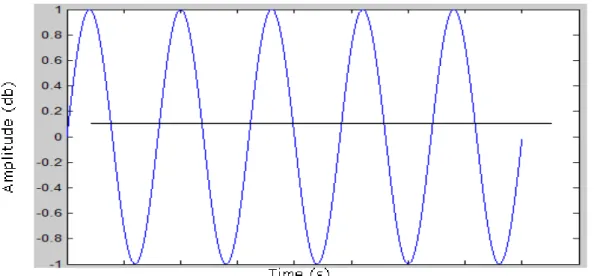
A sound is generated when something causes a disturbance in the density of gas, liquid or solid. These disturbances can be represented graphically as illustrated in figure 2.1.

When those disturbances reach humans’ ears, the brain converts them into electric

signals that travel along the brain and allow us to recognize sounds (as well as localize sounds sources, etc.).

Figure 2.1: A sound wave example. The signal can be represented as a waveform, where

17

Our goal is to process these audio signals in computers as we want to build a sound recognizer. Therefore, we have to see how we create the digital audio signal. Converting the audio signal from analog to digital, involves two processes: sampling and quantization. Sampling consists in storing the values of the wave at certain time instants. Each value stored is a sample point. After sampling is done, it returns a finite set of values. These values are rounded and converted to a 𝑘 bit number. This is called quantization. Using a low number of bits can produce higher quantization errors as the true amplitude values are further from their digital representation. By combining these processes it is possible to transform audio into a binary format that can be used in the computer.

After the sound wave is digitized it can be processed in order to obtain more information about the sound. This section discusses some sound processing techniques: Discrete Fourier Transform (DFT), Discrete Wavelet Transform (DWT) and Discrete Cosine Transform (DCT).

Fourier Transform converts a one variable function in another variable function. It is used to transform the time-varying waveform obtained after digitizing the sound into a frequency-varying spectrum more convenient to study the sound properties.

If the input function is discrete and its non-zero values have a limited duration we can call this operation Discrete Fourier Transform (DFT). DFT transforms the time domain amplitudes sequence 𝑥₀,𝑥1,…,𝑥𝑁−1 into the frequency domain amplitudes sequence

18

𝑋𝑘 = 𝑥𝑘 ∗ 𝑒−

2𝜋𝑖 𝑁𝑘𝑛 𝑁−1

𝑘=0 ,𝑘= 0,…,𝑁 −1 (𝑒𝑞 2.1)

This shows that sounds can be represented as a sum of 𝑁 sinusoidal components. These components describe the spectral characteristics of the sound and they can be used in order to recognize sound sources.

However, we are interested in studying the sound in detail and Fourier transform may not be enough to detect highly localized information. Instead of applying the Fourier transform to the whole signal, we will cut the signal 𝑥 𝑡 into different sections, or windows, with a time based function and apply the DFT to each section. This process is called Short-Time Fourier Transform (STFT) and can be defined in equation 2.2 with 𝑁 being the number of sampled points and where 𝑤(𝑡) is the time based function (window function) and 𝑚 and 𝜔 are the instants of time and frequencies respectively.

𝑆𝑇𝐹𝑇 𝑥 𝑡 = 𝑋 𝑚,𝜔 = 𝑥 𝑘 ∗ 𝑤 𝑘 − 𝑚 ∗ 𝑒−𝜔𝑘𝑖 𝑁−1

𝑘=0

(𝑒𝑞 2.2)

The result of STFT can be represented as a matrix 𝑆 where 𝑎_𝑓𝑡 is the amplitude at

instant 𝑡 ∈{0,…,𝑇} and frequency 𝑓 ∈{0,…,𝐹} (equation 2.3).

𝑆=

𝑎00 … 𝑎0𝑇

⋮ ⋮

𝑎𝐹0 ⋯ 𝑎𝐹𝑇

(𝑒𝑞 2.3)

19

color of each point in the image. For instance, figure 2.2 shows a spectrogram of a sound sampled from a staccato violin sound. The rows in the image are the frequency bins (higher frequencies have shorter duration). The brightness of the image points indicates the amplitude values (higher amplitude if brighter).

Figure 2.2: Extracted from [11], spectrogram from a staccato violin sound.

There is a tradeoff between the temporal and spectral representation given by the STFT related to the window function. A long window length provides a more detailed frequency representation. On the other hand, a short window provides a more detailed temporal representation and is, therefore, more appropriate for a time-analysis of the sound.

20

A one level transform of a signal 𝑥 𝑡 would be given by equations 2.4 and 2.5 where

𝑕 𝑡 and 𝑔 𝑡 are the high and low filter respectively.

𝑦𝑑𝑒𝑡𝑎𝑖𝑙 𝑡 = 𝑥 ∗ 𝑕 𝑡 = 𝑥 𝑘 ∗ 𝑕(2𝑛 − 𝑘) ∞

𝑘=−∞

(𝑒𝑞2.4)

𝑦𝑎𝑝𝑝𝑟𝑜𝑥𝑖𝑚𝑎𝑡𝑒 𝑡 = 𝑥 ∗ 𝑔 𝑡 = ∞𝑘=−∞𝑥 𝑘 ∗ 𝑔(2𝑛 − 𝑘) (𝑒𝑞 2.5)

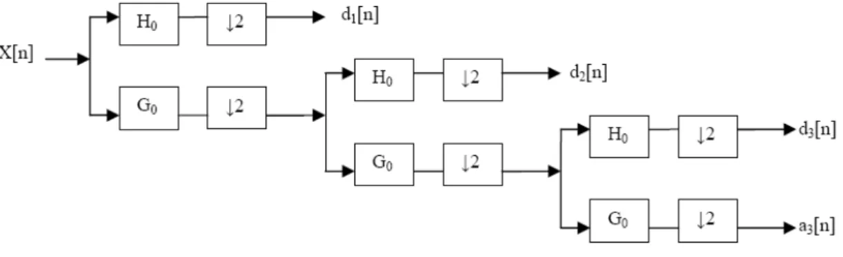
For instance, we can see a three-level wavelet decomposition tree in figure 2.3. 𝑋 𝑛 is the sound signal, 𝐻₀ the high filter and 𝐺₀the low filter. ↓ 2 is the operation that retrieves the detail coefficients 𝑦_{𝑑𝑒𝑡𝑎𝑖𝑙}(𝑡) (𝑑₁ 𝑛 ,𝑑2 𝑛 ,𝑑3 𝑛 ) and the approximate

coefficients 𝑦_{𝑎𝑝𝑝 𝑟𝑜𝑥𝑚𝑎𝑡𝑒} (𝑡) (𝑎3 𝑛 ).

Figure 2.3: Three-level wavelet decomposition tree.

21

The points 𝑥₀,𝑥₁,…,𝑥_𝑁−1 of the signal are transformed into 𝑋₀,𝑋₁,…,𝑋_𝑁−1as shown by equation 2.6 where 𝑁 is the number of sampled points.

𝑋𝑘 = 𝑥𝑛 ∗cos _𝑁𝜋 (𝑛 +

1

2)(𝑘+

1

2)

𝑁−1

𝑘=0

22

3. State of Art

There are two main factors that change the accuracy rate in sound recognition: the sound features used and the classification algorithm implemented. This section is divided in two parts: one that describes the progress in sound features extraction and another that describes the classification methods.

Sound Features Extraction

23

Features derived from volume contour describe the temporal variation of the sound’s

magnitude. The volume value depends on the recording process. However, the temporal variation of its value reflects properties of the sound useful for sound recognition. Features derived from pitch contour describe the fundamental period of the sound. As an instance, these features can be used to distinguish voice samples from music samples which, usually, have a longer period than speech samples. Finally, there are frequency domain features which describe the frequency variation of the sound. These features can be extracted with Fourier Transform.

24

Figure 3.1: Extracted from [12], three different type features of the same sound. On top the waveform of the sound. On bottom from left to right: the volume variation, the pitch

variation and the frequency centroid variation of the sound.

There are several algorithms to extract these features [13]. Even though, there are several approaches in audio feature extraction, most of them compute spectrograms to extract the features. Consequently, these are short-time features. However, selecting what features to use in sound recognition is not a closed topic.

There are several proposals of what features to use. Scheirer et al. developed a sound recognizer [14] which used a set of 8 features:

 4 Hz modulation energy

 Percentage of “Low-Energy” Frames

 Spectral Rolloff Point

news waveform

25

 Spectral Centroid

 Spectral “Flux” (Delta Spectrum Magnitude)

 Zero-Crossing Rate (ZCR)

 Cepstrum Resynthesis Residual Magnitude

 Pulse metric

Analyzing some of these features may make other good features. The variances of the derivative of Spectral Rolloff Point, of Spectral Centroid, of Spectral “Flux”, of Zero -Crossing Rate and of Cepstrum Resynthesis Residual Magnitude can be used as features, too.

As described in Table 3.1, each feature can be tested to find its usefulness. Although some features alone show a big error rate (for instance, note that Spectral Rolloff Point has an error rate of almost 50%), using the features all together provided great results (around 90% accuracy).

26

Other recognizer using short-time features was proposed by Eronen et al [15]. This recognizer used and tests separately a set of 10 features:

 Zero-crossing rate

 Short-time average energy

 Band-energy ratio

 Spectral Centroid

 Bandwidth

 Spectral roll-off point

 spectral flux

 Linear prediction coefficients,

 Cepstral Coefficients

 Mel-frequency cepstral coefficients (MFCC)

When the features were tested, MFCCs provided the best recognition rate (above 60%). This is not the only example where MFCCs out-perform other features. In fact, MFCCs are very popular in sound recognition. They consist of a set of coefficients that make a short-term power spectrum of a sound, just like what is done by the Fourier Transform. However, while the Fourier Transform uses the Hertz scale, MFCCs use the Mel scale, which has frequency bands that are not equally spaced (in similarity to what happens in the human ear).

27

These features were tested in a recognizer [16] which has the purpose of distinguishing scenes (popular music, classic music, speech, noise and crowd). The results showed they could out-perform MFCCs: Figures 3.2 and 3.3 show the classification result for each scene using MFCCs and the classification results using Filterbank envelopes respectively. We can see they provide better results in classes more related to speech sounds (noise, crowd). In classical music, MFCCs still provide much better results than these features.

Figure 3.2: Extracted from [16], accuracy results provided by MFCCs.

28

Other works process audio using Wavelet Transform (WT) instead of Fourier Transform. This results in different features as STFT transforms the sound in a spectrogram and WT decomposes the sound in various functions, as mentioned before in section 2. These features are extracted from these functions and were tested against MFCCs and short-time features. Figure 3.4 shows how MFCCs are more useful in sound recognition. While short-time features are comparable to the wavelet features, MFCCs retrieves higher recognition rates in every class tested.

Figure 3.4: Extracted from [17], the accuracy results from wavelet features (DWTC) against MFCC and short-time features (FFT).

29

 Audio Waveform – description of the shape of an audio signal

 Audio Power – temporal descriptor of the evolution of the sampled data  Audio Spectrum Envelope – series of features that describe the basic spectra

 Audio Spectrum Centroid – center of the log-frequency spectrum’s gravity

 Audio Spectrum Spread – measure of signal’s spectral shape

 Audio Spectrum Flatness – measure of how flat a particular portion of the signal

is

 Harmonic Ratio – proportion of harmonic components in the power spectrum

 Upper Limit of Harmonicity – measure of the frequency value beyond which the

spectrum no longer has any harmonic structure

 Audio Fundamental Frequency – estimation of the fundamental frequency

30

Table 3.2: Extracted from [18], the accuracy obtained with MFCCs (on the left) and with MPEG-7 descriptors (on the right).

To provide better recognition rates some improvements over MFCCs [19] have been done, too. ICA can be applied over these features. The result features showed ICA transformation is useful in sound recognition [20]. One good example is a sound recognizer based on kitchen events (water boiling, vegetable cutting, microwave beep, etc.) [21]. ICA was tested and also improved the accuracy results (Table 3.3) from 80.6% to 85% as we can see in table 3.6.

System Error Precision BASE 12.4% 80.6%

ICA 9.2% 85.0%

31

Both ICA and PCA are not fully explored in environmental sound recognition. Instead of being applied only to the set of MFCCs, these techniques could be applied to the whole spectrogram retrieving new features that can be used. In speech recognition there are examples of how ICA and PCA can provide better results. In [22], the sound features were extracted applying ICA to spectrograms which were computed to represent the speech samples. The number of features extracted influences the results. However, we can see in Table 3.4 how features extracted with ICA could out-perform MFCCs: using only 20 or 30 basis functions extracted with ICA as features provides a lower error rate than using MFCCs.

Table 3.4: Extracted from [22], the error rates of feature extraction with ICA against MFCCs.

32

Sound Recognition and Classification

Above, we have seen several approaches in sound feature extraction. After extracting these features, it is necessary to implement a classification algorithm that uses the features to match the tested sounds to the right category. This section discusses some sound recognizers focusing on the techniques they use for classification.

33

Table 3.5: Table extracted from [24]. The accuracy rates of the recognizer using FilterBank and k-NN.

A recurrent neural network (RNN) was also used to classify these sounds but with very poor results, which shows that the k-NN is more appropriate for these classes. The implemented RNN uses RASTA (Relative Spectral Transform) coefficients which are useful in speech recognition and are short-time features. The maximum recognition rate returned was 73.5% using the data used to train the RNN. Using other data that would fit in the classes used, the recognition rate was 24% which is a very poor result.

34

Table 3.6 shows the music error rate, the speech error rate and the total error rate of both methods. We can see MPN provides much lower error rates. Although the Bayesian Classifier is a simple algorithm, the difference in the music error rate is considerable, which shows that the MPN is more appropriate to classify these sounds.

Table 3.6: Extracted from [25], Error Rates returned by the MPN network (first row) and by ZCR with the Bayesian Classifier (second row).

35

Table 3.7: Extracted from [26]: the error rates retrieved by the each classification method using different sets of features: a set of short-time features (Perc) and a set of k MFCC’s (CepsK).

Support Vectors Machine (SVM) is another alternative to the k-NN algorithm. This was tested using five classes of sounds (silence, music, background sound, pure speech, non-pure speech) [27]. However, we can only apply SVM if we use only two classes each time. In order to do this, the silence class was separated from the others 4 classes (non-silence). Figure 3.5 shows how these other four classes were divided.

36

Therefore, SVM is not a very practical method for environmental sound recognition, especially if using several sound classes. However, it can provide impressive recognition rates as shows Table 3.8: all the accuracy rates are higher than 90%.

Table 3.8: Extracted from [27], sound classes division for multi-class classification using SVM.

Other alternative to these techniques consists of using Gaussian Mixture Models (GMM). GMM consists in modeling a new cluster for each of the studied classes using its information. Assuming a cluster is denoted by𝑦_𝑘, each one of them will have a related function𝑝 𝑥 𝑦_𝑘 . Assuming 𝑁 is the number of clusters generated, the classification algorithm assigns the cluster 𝑦_𝑘 to the tested object 𝑥 if

𝑦𝑘 = arg max1 ≤𝑖≤𝑁𝑝(𝑥|𝑦𝑖)

37

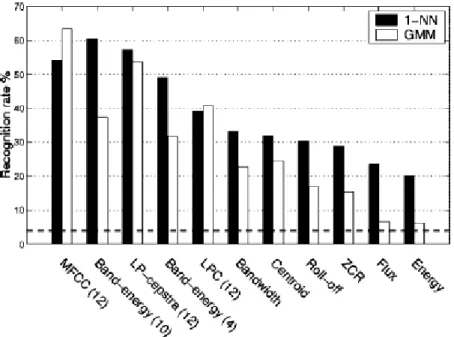
Comparing the different features used and the classification methods, GMM classifier provides better recognition accuracy (63.4%) when using MFCCs. Considering MFCCs were proven to be very useful in sound recognition, GMM consists in a good technique for sound classification (figure 3.6).

Figure 3.6: Extracted from [15], features’ recognition rate with two different classifiers

GMM and 1-NN.

38

Instead of a k-NN or a GMM, a hidden Markov Model (HMM) can also be used as the classification framework. An HMM consists of a set of states and the probabilities of changing from each state to each of the other states. The probability of observing a sequence of states

𝑌 = 𝑆_𝑎,𝑆_𝑏,𝑆_𝑐,𝑆_𝑑

is given by

𝑃 𝑌 = 𝑃(𝑌|𝑆_𝑖 𝑁

𝑖=0

)𝑃 𝑆_𝑖

where 𝑁 is the number of states.

Now it is necessary to adapt the HMM to the sound classification problem. Each class 𝑣 is modeled into a HMM 𝜆𝑣 using the features extracted. For matching the tested sample with one of the classes, the recognizer identifies the sequence of states

𝑂 = 𝑆_𝑥… 𝑆_𝑦

using its sound features and assigns it to the class 𝑣 if

𝑣= arg max

1 ≤𝑣≤𝑉𝑝(𝑂|𝜆

𝑣₎

39

The overall accuracy obtained with ten different environments was 91.5%. The same test was done with persons resulting in a 35% accuracy which can be justified by the short samples used in the test. However, the number is much smaller than the obtained by the HMM model. As we can see, combining MFCCs and HMM can provide great results (figure 3.7): in four different contexts the recognition rate was 100%. However, note that street context has a lower recognition rate of 75%. This happens because these sounds are similar to the Rail Station, the lecture and the car context sounds and similar sounds make the recognizer task harder.

Figure 3.7: Extracted from [28], recognition rates of 10 contexts using HMM.

40

Figure 3.8: Extracted from [29], the comparison of recognition rates for 18 contexts.

In this same work, discriminative training was tested. Discriminative training adjusts the parameters of the HMMs assigning rules to reduce the error rate in recognition. However, it did not improve the accuracy obtained. On the other hand, discriminative training for the classification process was also tested by Eronen in 2003 [18] showing minimal improvements.

41

42

4. Proposed Solution

Sound recognizers have to perform three steps to achieve their goal (figure 4.1). First, the sound has to be digitized and processed; it is transformed into a representation that is suitable for the extraction of features from its new digital representation. The next step consists of extracting the chosen audio features. Finally, these features will be used in the last step where the sound is classified (assigned to a class).

Figure 4.1: The three steps of an environmental sound recognizer.

The data used to test the proposed similar sound recognizer is a set of impacts on rods [6], which includes samples from four rods with the same length and diameter but different materials (wood, aluminum, steel and zinc plated steel). The sounds were all produced by impacts on the same region of the rod (close to the edge). Even though the

Audio Digitization and processing

Audio features extraction

43

sounds differ from each other due to variations on the impact force and on the location of impact, they are quite similar as they are produced by the same type of event and by objects with the same shape and size which only differ in material. The first step of our classifier consists of digitizing the sounds, which was already accomplished in [6] with a sampling frequency of 44100 Hz, and representing them with spectrograms so that they are ready to be used by the next step of the recognizer.

The next step (second stage of figure 4.1) consists of extracting the sound features. Instead of extracting pre-defined features of the sounds such as MFCCs or short-time features, our recognizer learns them from the data. In order to learn the features, the recognizer uses the Intrinsic Structures Analysis (ISA) method, which in turn uses Independent Component Analysis (ICA) and Principal Component Analysis (PCA) of the spectrogram of the sounds [6]. Here we prove that the features learned in this manner are powerful enough for sound classification of very similar sounds. These techniques allow us to extract time and frequency-varying functions that we use as features for classification in the third stage of the classifier (the third box in figure 4.1).

The final step is to classify the sound. We use the features extracted with the ISA method in a 1-Nearest Neighbor Algorithm as we mentioned in the end of section 3 and explain it with detail below. We can see these three steps in figure 4.2.

Figure 4.2: The three steps of the proposed sound recognizer. Audio Digitization

and processing with STFT

Audio features extraction with the

ISA

Sound classification with

44

The remaining of this section is divided in two parts. First, we describe both ICA and PCA techniques and the features we will extract after representing the sounds with spectrograms. Then, we describe the classification method.

1. Features extraction with the ISA method

The ISA method uses spectrograms as the initial representation of the sounds and extracts features from the spectrograms. It proposes two different ways of using the spectrogram (either the original spectrogram or the transpose) along with two distinct techniques to analyze them (ICA and PCA). We will use all these combinations separately and then compare the results obtained by each technique.

ICA [30, 31] is a technique to separate mixed source signals from signal mixtures.

Given a matrix S containing the signal mixtures, ICA’s goal is to find the matrix W so

that the rows of X, the source signals, are the most independent possible:

𝑋=𝑊𝑆

𝑆=𝑊−1𝑋=𝐴𝑋

As we have seen, the STFT of a sound S is a matrix of amplitudes 𝑎_𝑓𝑡. By assuming

that S consists of a set of signal mixtures, ICA is able to separate the source signals by learning a matrix A that verifies

𝑆=𝐴𝑋

𝑎00 … 𝑎0𝑇

⋮ ⋮

𝑎𝐹0 ⋯ 𝑎𝐹𝑇

=

𝛼0 … 𝛾0

⋮ ⋮

𝛼𝐹 ⋯ 𝛾𝐹

𝑥00⋮ … 𝑥0⋮𝑇 𝑥𝑁0 ⋯ 𝑥𝑁𝑇

45

This separation is done by representing each column of A as an orientation vector (i.e. basis function) of the correspondent line of X so that

𝑎𝑖0… 𝑎𝑖𝑇 = Ai T𝑋

*

𝑎𝑖0… 𝑎𝑖𝑇 = 𝛼𝑖… 𝛾𝑖

𝑥00 … 𝑥0𝑇

⋮ ⋮

𝑥𝑁0 ⋯ 𝑥𝑁𝑇

𝑎𝑖0… 𝑎𝑖𝑇 =𝛼𝑖 𝑥00… 𝑥0𝑇 + …+ 𝛾𝑖 𝑥𝑁0… 𝑥𝑁𝑇

where a_it is the inner product of the vector A T_i = 𝛼_𝑖… 𝛾_𝑖 and the ith column in X:

x0i… xNi T .

Just like ICA, PCA [30, 32] also decomposes S into matrixes A and X. The main

difference is that PCA’s goal is not to find a matrix W such that the rows of X are

independent but uncorrelated.

The rows of X, the source signals, are the values of the features we will use for classification. They can be seen as time-varying functions (figure 4.3, left column) each one with an associated orientation vector. This vector can be seen as a frequency-varying function (figure 4.3, right column).

*

46

Figure 4.3: Temporal features extracted with ICA from a wood sound (left column: source signals xi0… xiT ; right column: the associated orientation vector δ0… δF T ).

As ICA and PCA are matrix operations we can perform them over the transpose of the

sound’s spectrogram

𝑆𝑇 _=𝐴𝑋

𝑎00 … 𝑎0𝐹

⋮ ⋮

𝑎𝑇0 ⋯ 𝑎𝑇𝐹

=

𝛼0 … 𝛾0

⋮ ⋮

𝛼𝑇 ⋯ 𝛾𝑇

𝑥00⋮ … 𝑥0⋮𝐹 𝑥𝑁0 ⋯ 𝑥𝑁𝐹

where ai0… aiF is a signal mixture and xi0… xiF is a source signal and 𝑁 ≤ 𝑇. The

47

Figure 4.4: Spectral features extracted with ICA from a wood sound (left column: source signals 𝑥i0… 𝑥F ; right column: associated orientation vector δ0… δT T).

48

1. Sound classification with 1-NN

The third stage of our classifier (figure 4.2) uses a 1-Nearest Neighbor algorithm. In order to implement this algorithm, we need to build a training data set. Once that is done, the algorithm is ready to classify test samples: it matches the test sample to one record of the training data set based on the Euclidean distance. It just sees which training data sample is the closest to the tested sample. The tested sample is assigned the class that occurs more in the 𝑘 neighbors (1 in our case).

The classification method of our recognizer is described by figure 4.5. Our training data is composed of the coefficients associated to 𝑀 orientation vectors of 𝑁 sounds (𝑁/4

sounds for each of the four classes we have). Each record in the training data set consists of those 𝑀 coefficients from one sound (figure 4.5). The tested sample is composed by the 𝑀 coefficients associated to the same orientation vectors.

Then, using 1-NN, we compare the value of the 𝑀 coefficients in one instant of time or frequency (depending on the analysis) of the training sample

(𝐶₁𝑇𝑟𝑎𝑖𝑛𝑖𝑛𝑔 𝑆𝑎𝑚𝑝𝑙𝑒,𝐶₂𝑇𝑟𝑎𝑖𝑛𝑖𝑛𝑔 𝑆𝑎𝑚𝑝𝑙𝑒 ,…,𝐶_𝑀−𝑇𝑟𝑎𝑖𝑛𝑖𝑛𝑔₁ 𝑆𝑎𝑚𝑝𝑙𝑒,𝐶_𝑀𝑇𝑟𝑎𝑖𝑛𝑖𝑛𝑔 𝑆𝑎𝑚𝑝𝑙𝑒 )

with the 𝑀 coefficient values of the test sample

(𝐶₁𝑇𝑒𝑠𝑡,𝐶₂𝑇𝑒𝑠𝑡 ,…,𝐶_𝑀−𝑇𝑒𝑠𝑡₁,𝐶_𝑀𝑇𝑒𝑠𝑡)

The 1-NN algorithm computes the Euclidean distances between the test sample and all training samples and returns the index of the training sample which is closest to the test sample:

𝑖 = arg min_{1 < 𝑖 <𝑁} 𝑋 (𝐶_𝑥𝑇𝑒𝑠𝑡 − 𝐶_𝑥𝑇𝑟𝑎𝑖𝑛𝑖𝑛𝑔 𝑆𝑎𝑚𝑝𝑙𝑒 𝑖)2

49

with 𝑁 being the number of sounds in the training data and 𝑀 the number of used features. We repeat this process for various instants of time or frequency (depending on the analysis). The final class assigned to the tested sound is the one which occurs more in the instants selected.

Figure 4.5: Classification scheme of our recognizer.

.

.

.

.

.

.

Sound (zinc plated steel)

.

.

.

.

.

.

0 0.5 1 1.5 -5 0 5 Time (seg) A m p li tu d e ( d B ) Coeficiente 1

0 0.5 1 1.5

-20 0 20 Time (seg) A m p lit u d e ( d B ) Coeficiente 1

0 0.5 1 1.5

-5 0 5 Time (seg) A m p lit u d e ( d B

) _{Coeficiente 1}

0 0.5 1 1.5

-5 0 5 Time (seg) A m p lit u d e ( d B ) Coeficiente M

0 0.5 1 1.5 -10 0 10 Time (seg) A m p lit u d e ( d B ) Coeficiente M

0 0.5 1 1.5

50

5. Implementation

As discussed before, the implemented recognizer is divided in three phases. The first phase consists of transforming the data from a time representation (that is, from waveforms) into a spectrotemporal representation (which is suitable to be used in the next phase of the recognizer). This consists of taking the spectrograms of the sounds and concatenating them into a unique matrix. Then, the second phase consists of learning features that will later be used in a recognition algorithm. The features are learned by either ICA or PCA of the concatenated spectrograms. Finally, we use the features extracted by ICA or PCA for classification with the 1-NN algorithm.

51

 Building the training data

As mentioned above, the sounds are initially represented by spectrograms, which are obtained by the STFT function with a 512-Hanning window, 512-point FFT and 256 overlap. Figure 5.1 shows an example of a spectrogram from one of our sounds. This way, each sound is described by a matrix of frequency by time, i.e. an array of vectors

𝑓1,𝑓2,…,𝑓𝑡, with 𝑡 being the number of spectrogram frames (that can be thought of as

time instants) and 𝑓_𝑥 the vector with the frequency values in instant 𝑥. The spectrograms are then concatenated into a bigger matrix. The way this concatenation is made depends on whether we use temporal or spectral analysis (see section 4).

Let us first look into temporal analysis. In this case, the spectrograms, which have size 𝐹×𝑇 , are concatenated horizontally to obtain a bigger matrix of size 𝐹 × 𝑁𝑇

where N is the number of sounds, just as if the sounds were reproduced in sequence, one after the other. This bigger matrix is then used as input to ICA or PCA and we can see an example in figure 5.2.

Figure 5.1: The spectrogram of one of the sounds made by a steel rod.

F re q u e n c y ( H z ) Time (s) Spectrogram

0 0.2 0.4 0.6 0.8

0.5

1

1.5

52

Figure 5.2: Example of a matrix of spectrograms for temporal analysis: (𝑆1,𝑆2,𝑆3,𝑆4)∗.

This matrix contains four sounds, each one made by a different rod.

Now, let us look into spectral analysis. The spectrograms of size 𝐹×𝑇 are now concatenated vertically in order to compose a bigger matrix of size 𝑁𝐹 × 𝑇 . The transpose of the obtained spectrogram, with size 𝑇 × 𝑁𝐹 , is the matrix we use as input for ICA or PCA (figure 5.3).

Fig 5.3: Example of a transposed matrix of transposed spectrograms for spectral analysis: (𝑆1𝑇,𝑆2𝑇,𝑆3𝑇,𝑆4𝑇). This matrix contains four sounds, each one made by a different rod.

*

(A,B) is the horizontal concatenation of matrixes A and B.

Fr e q u e n c y ( H z ) Time (s) Spectrogram

0 0.5 1 1.5 2 2.5 3

0.5

1

1.5

2

x 104

F re q u e n c y ( H z ) Time (s) Spectrogram

0 0.1 0.2 0.3 0.4 0.5 0.6 0.7 0.8

0.5

1

1.5

2 x 104

53

The next step consists of applying ICA or PCA over the concatenated spectrograms described above. As explained above, ICA and PCA transform a matrix of mixed sources 𝑆 in a matrix of (estimated) source signals 𝑋 finding a transformation matrix 𝐴 where each column is the orientation vector of each row of the matrix𝑋:

𝑆= 𝐴𝑋

In our implementation the matrix 𝑆 is the matrix of concatenated spectrograms. ICA learns matrix 𝐴 and along with it, it returns matrix 𝑋. In particular, we use the fastICA algorithm, which is the Matlab ICA implementation by Hyvärinen et al. [33]. Each row of the matrix 𝑋 is the value of one of the extracted features, strictly speaking it has the concatenation of 𝑁 values of one of the extracted features, where 𝑁 is the number of sounds.

Figure 5.4 shows the values of one of the features obtained by temporal analysis with ICA. These values are arrays of amplitude varying over time until time instant𝑁𝑇. Figure 5.5 shows the values of one of the features retrieved with spectral analysis with ICA. These values can be seen as arrays of frequency-varying amplitude.

54

Fig 5.4: Values of an ICA feature obtained with temporal analysis over a spectrogram with 20 sounds (five from each class: aluminum in red, zinc plated steel in blue, wood

in green and steel in black).

Fig 5.5: Values of an ICA feature obtained with spectral analysis over a spectrogram with 20 sounds (five from each class: aluminum in red, zinc plated steel in blue, wood

in green and steel in black).

We use PCA like we use ICA because PCA also learns matrix 𝐴 to return matrix𝑋. To apply PCA we use princomp Matlab function. Like in ICA, each row of matrix X contains N values of one feature being N the number of sounds. One of these rows extracted with PCA for temporal analysis can be seen in figure 5.6 and one extracted with PCA for spectral analysis can be seen in figure 5.7.

Like with the ICA features, PCA features also allow us to distinguish some classes of the sounds immediately. In both figure 5.6 and 5.7, the aluminum sounds and the steel sounds have low amplitude values compared to the zinc platted steel sounds and the wood sounds.

0 2000 4000 6000 8000 10000 12000

-20 0 20 40 Time (s) A m p lit u d e ( d B )

0 1000 2000 3000 4000 5000 6000

-20 -10 0 10

Repeated Frequencies (Hz)

55

Fig 5.6: Values of a PCA feature obtained with temporal analysis over a spectrogram with 20 sounds (five from each class: aluminum in red, zinc plated steel in blue, wood

in green and steel in black).

Fig 5.7: Values of a PCA feature obtained with spectral analysis over a spectrogram with 20 sounds (five from each class: aluminum in red, zinc plated steel in blue, wood

in green and steel in black).

Then we have to build our training data using the matrix X which is returned by PCA or ICA. As we have seen, each record of our training data set consists of the selected coefficients of one of the 𝑁 sounds. To select the coefficients we sort the orientation vectors according to the percentage of variance they account for. We select some of the most dominant orientation vectors and use the corresponding coefficients to build the training data set. Sorting the orientation vectors is an easy task for PCA but hard for ICA as the orientation vectors are perpendicular with PCA but not with ICA (that is, with PCA the inner product is zero while it may be different from zero with ICA), which means that it is hard to know how much of the variance of the data one orientation vector from ICA accounts for.

0 2000 4000 6000 8000 10000 12000

-2 0 2 Time (s) A m p lit u d e ( d B )

0 1000 2000 3000 4000 5000 6000

-2 0 2 4

Repeated Frequencies (Hz)

56

0 2000 4000 6000 8000 10000 12000

-2 0 2 Time (s) A m p lit u d e ( d B )

0 2000 4000 6000 8000 10000 12000

-10 -5 0 5 Time (s) A m p lit u d e ( d B )

To build the training data set we will group the values for the 𝑀 features of each sound as is illustrated in figure 5.8: we will build 𝑁 matrixes with size 𝑀×𝑇 for temporal analysis or 𝑁 matrixes with size 𝑀×𝐹 for spectral analysis. Each matrix built is one record of the training data set.

Figure 5.8: A set of 10 features extracted with PCA for spectral analysis and how we use it to build the training data set.

0 2000 4000 6000 8000 10000 12000

57  Classification of the tested data

To classify a sound from the test data set, we do not need to perform ICA or PCA over its spectrogram and compare the obtained features with the ones from our training data. Instead, we use the orientation vector matrix that was previously learned by ICA or PCA (that is, matrix 𝐴).

As we have seen after performing ICA and PCA we obtain two matrixes 𝐴 and 𝑋 and we use sub matrixes 𝐴’ and 𝑋’ to build the training data set:𝐴′ of size (𝐹 × 𝑀), and 𝑋′ of size (𝑀 × 𝑁𝑇) with 𝑀 being the number of used features.

𝑆 = 𝐴 ∗ 𝑋

𝐹 × 𝑁𝑇 𝐹 × 𝑀 𝑀 × 𝑁𝑇

Now, let’s assume 𝑆1 is our test sound spectrogram instead of the spectrogram of all the

training sounds

𝑆1 =𝐴 ∗ 𝑋1

𝐹 × 𝑇 𝐹 × 𝑀 𝑀 × 𝑇

𝐴−1𝑆1 =𝐴−1∗ 𝐴 ∗ 𝑋1

58

𝑋1 is the matrix with the features represented according to the orientation vectors

stored in matrix 𝐴 (that was learned by ICA or PCA of the training data). The obtained matrix 𝑋1 is the one we use for classification.

As we have seen, each record of our training data is a matrix 𝑀 × 𝐹 or 𝑀 × 𝑇 just like the matrix we obtained above. Each column of this matrix represents the value of M features in one instant of time or for one frequency bin depending on the analysis (spectral or temporal) we are using.

59

Fig 5.9: Temporal feature extracted with ICA of an aluminum sound (left) and one wood sound (right). In red, the instants we use in the classification.

Fig 5.10: Spectral feature extracted with ICA of an aluminum sound (left) and one wood sound (right). In red, the frequency bins we use in the classification.

The 1-NN algorithm compares each (tested) column of the matrix 𝑋1 obtained for the test sample with the respective columns of the 𝑁 records of the training data set. For each tested column, the algorithm returns the index of the training record whose column is nearer the one obtained for the tested sound. Each training record has a class assigned. The class that occurs more often in the amount of columns we use is the one assigned to the tested sound.

0 1 2 3 4

x 10-3 -10 0 10 20 A m p lit u d e ( D b ) Time (s)

0 0.5 1 1.5 2

x 104 -10 -5 0 5 Frequency (Hz) A m p lit u d e ( D b )

0 1 2 3 4

x 10-3 -5 0 5 10 Time (s) A m p lit u d e ( D b )

0 0.5 1 1.5 2

60

6. Result Analysis

We have conducted several experiments to test our recognizer. In this section we analyze the results obtained after doing both spectral and temporal analysis with both ICA and PCA. In the end, we validate our results: we test our recognizer with MFCCs and compare the results with the ones we obtained with our features.

Our data consists of 18 sounds of aluminum, 15 of zinc plated steel, 16 of wood and 15 of steel. We build two training sets for all analysis we perform: one with 20 sounds (five of each class) and one with 40 sounds (ten of each class). The remaining sounds are the sounds we use to test our recognizer.

 ICA – Temporal Analysis

61  ICA – Spectral Analysis

The results of spectral analysis with ICA can be seen in figure 6.2. We obtained rates of 100% for aluminum and zinc plated steel sounds, 73% for wood sounds and 60% for steel sounds with the smaller training set. On the other hand, we obtained rates of 83% for wood sounds and 100% for the rest of them when using the bigger training set.

Fig 6.1: Temporal analysis with ICA results.

Fig 6.2: Spectral analysis with ICA results. 0

20 40 60 80 100 120

20 Sounds 40 Sounds

Aluminum

Zinc plated Steel

Wood

Steel

0 20 40 60 80 100 120

20 Sounds 40 Sounds

Aluminum

Zinc plated Steel

Wood

62

If we compare the spectral analysis results with the temporal analysis results we see the difference is minimal. When using the bigger training set the results are overall the same. The difference is that, in temporal analysis, one sound of zinc plated steel is not well recognized (which results in a recognition rate of 80% for this rod) and in spectral analysis this happens with a wood sound (which results in recognition rate of 83% for this rod). When using the smaller training set, we only get 100% recognition with wood sounds when doing temporal analysis. We suspect that the temporal functions from the other rods have more similarities and are harder to distinguish. If we look at the spectral analysis results, we get a recognition rate of 100% in both aluminum and zinc plated steel sounds. However, the rates for wood and steel sounds are smaller. We only got 60% for the steel sounds as the recognizer classified 40% of the steel sounds as aluminum instead. Nonetheless, the overall results are excellent and show how powerful the features extracted with ICA can be for similar sound recognition.

 PCA – Temporal Analysis

The results of temporal analysis with PCA are shown in figure 6.3. When using the smaller training set, we obtained recognition rates of 100% for all sounds except for steel sounds where we get 70% rate. When using the bigger training set, the rates are always 100%.

 PCA – Spectral Analysis

63

using the bigger training set, the rates are 100% for all materials except for wood sounds where we obtain a recognition rate of 83%.

Fig 6.3: Temporal analysis with PCA results.

Fig 6.4: Spectral analysis with PCA results. 0

20 40 60 80 100 120

20 Sounds 40 Sounds

Aluminum

Zinc plated Steel

Wood

Steel

0 20 40 60 80 100 120

20 Sounds 40 Sounds

Aluminum

Zinc plated Steel

Wood

64

The results from both spectral and temporal analysis with PCA are very similar. When using the bigger training set, we get an overall recognition rate of 100% with temporal analysis and only one wood sound was not well recognized with spectral analysis (retrieving a recognition rate of 83% for this rod).

When using the smaller training set, we registered three steel sounds badly recognized with temporal analysis. On the other hand, when we performed spectral analysis our recognizer failed to classify three sounds as well: one of zinc plated steel, one of wood and one of steel.

Comparing these results to the ICA results, the difference is minimal. The overall results show PCA provided slightly better rates. We suppose this happens because when selecting the ICA set of features we use, we sort it by variance and use the first ones. Instead, we could find the features that describe the difference between the materials and we suppose we could retrieve better results even using fewer features than the ones we use. However, the main conclusion these results allow us to make is that both ICA and PCA are really powerful techniques to extract sound features.

65

 MFCCs

As previously mentioned, MFCCs are very popular in sound recognition. MFCCs consist in a set of coefficients that describe the power spectrum of a sound. Since MFCCS are so popular and we want to see which features perform better, we used MFCCs with our data to compare their results with those obtained with our features.

The results of replacing our features by MFCCs in our recognizer are shown in figure 6.5. We use the kannumfcc Matlab function [34] and extract 11 coefficients which we use in our recognizer. When using the smaller training set, we obtained recognition rates of 83% for aluminum sounds, 70% for zinc plated steel sounds, 64% for wood sounds and 50% for steel sounds. When using the bigger training set, the rates are 100% for all aluminum and zinc plated steel sounds while we get a rate of 67% for wood sounds and 60% for steel sounds.

Fig 6.5: Results using MFCCs. 0

20 40 60 80 100 120

20 Sounds 40 Sounds

Aluminum

Zinc plated Steel

Wood

66

MFCCs with the lower training set provide a low overall recognition rate of 66.75%. We can see clearly that increasing the training set provides much better results. However, even with the bigger training set the results obtained with MFCC are lower than any other analysis we previously performed.

Fig 6.6: Overall recognition rates provided by all the analyses made.

Figure 6.6 shows the comparison of all the analysis made. The temporal analysis with PCA retrieves the best results achieving 100% recognition in all four classes of sounds we have. The other three analyses we performed only were mistaken in one sample when using a training set of 40 sounds. Even with a smaller training set of 20 sounds, both temporal and spectral analyses retrieved an overall recognition above 83% when using ICA and above 90% when using PCA.

83,95 92,75 90,5

92,5

66,75

95,75 95,75 95 100

81,75 0 20 40 60 80 100 120

67

Compared to the results we obtained using MFCCs, any of our features set is much better. MFCC with the bigger training set only returns an overall recognition rate of 81,75% which is smaller than any recognition rate any analyses (even with the smaller training set) we made before provided.

68

7. User Study

As seen in the previous section, the proposed recognizer gives excellent recognition rates, which are even higher than those obtained when we substitute the features learned by the ISA method by MFCCs, which, as mentioned above, are very commonly used in tasks of this nature. A natural question that follows is if the recognizer can surpass human ability to classify similar sounds and if the sounds are actually hard to distinguish. To answer these questions, we conducted two user studies.

69

 Protocol 1 – user study without feedback

Before the actual test starts, the users hear two sounds of each of the four classes (aluminum, steel, zinc plated steel and wood). A dialog box (figure 7.1) is presented that indicates the type of sound that is going to be played and that guarantees that the users only hear the sound when they are ready. In order to have no presentation order effects, the order of presentation of the sounds varies so that different subjects can hear the sounds in different orders but the sounds from the same class are always presented consequently. For example, the user may first listen to two aluminum sounds, then two wood sounds, etc. or he/she may first hear two steel sounds, then two aluminum sounds, etc. The same sounds were used for all subjects.

Figure 7.1: Dialog box for the first listening samples

70

Figure 7.2: Dialog box to listen to the train and test samples

Figure 7.3: Dialog box to identify the material that caused the heard sound

Then the actual test begins with the same dialog boxes (figures 7.2, 7.3). The subjects heard 41 sounds present in random order and with no repetitions: 7 of aluminum, 11 of zinc plated steel, 12 of wood and 11 of steel. The sounds presented are the same for all tests done, only the order of presentation differs. The study is performed in a laptop using headphones.

 Protocol 2 – user study with feedback

71

Like before with protocol 1, first the users heard two sounds from each class. Also like before, they were explained that in the next stage they would hear sounds from the same four classes that they heard in the first part of the test and that they had to identify the class of the sound. They are presented 12 training trials but here they receive feedback on whether their answers were correct or wrong: the subjects heard 12 sounds (three from each class) and tried to identify the class of the rod which caused the sound (figures 7.2 and 7.3). After the user identifies the class, a dialog box (figure 7.4) pops up

with the answer: “correct” if the user identifies the class with success or “wrong” with

the right answer otherwise.

Figure 7.4: Dialog box with the right answer during the training samples.

72

 Results

The first user study we conducted had 12 participants with ages between 23 and 55. None had hearing problems and two had acoustics knowledge. The results can be seen in table 7.1.

Aluminum Zinc plated steel Wood Steel

Aluminum 22.619% 53.571% 0% 23.81%

Zinc plated steel 43.939% 24.242% 0% 31.818%

Wood 1.3889% 0% 97.917% 0.69444%

Steel 28.03% 25.758% 0% 46.212%

Table 7.1: The table of answers of our first user study. Each row states the answers obtained for each material.

73

25.758% were zinc plated steel. Like with aluminum and zinc plated steel sounds, none of the wrong answers of the steel sounds were wood.

The second user study we conducted provided better results as the users had more

“training” than in the first user study. We had 11 participants with ages between 23 and

50. None had hearing problems and one had a high level of acoustics knowledge. The results are shown in table 7.2.

Aluminum Zinc plated steel Wood Steel

Aluminum 53.247% 23.377% 0% 23.377%

Zinc plated steel 26.364% 40.909% 0% 32.727%

Wood 0% 0% 100% 0%

Steel 27.273% 28.182% 0% 44.545%

Table 7.2: The table of answers of our second user study. Each row states the answers obtained for each material.

74

 Result Analysis

The results show that the sounds used in this dissertation are very hard for humans to distinguish. The low percentage of right results for aluminum and zinc plated steel sounds registered in the first study made us do a new user study with more training for the users. The results improved for these materials in the second study. The percentages of right answers are inferior to 55%, though. This shows how hard it was for the users to distinguish the metal sounds. The random order of the sounds during test also influences the results because people tend to forget the characteristics of the sounds they memorized before.

The mistaken answers also reveal that the sounds are so similar. For instance, in the second study, when missing the aluminum answer, we detect the same percentage of wrong answers for steel and zinc plated steel. The users assume it can be any of the three metals when confused.

75

The percentage of steel sounds recognition was much higher than the percentage of right answers for aluminum or zinc plated steel in the first user study. However, it did not improve in the second user study where users got more training.

We did register in the second user study, one test where the user had a high knowledge of acoustics. He only missed six answers out of thirty-two: three zinc plated steel sounds and three steel sounds. This shows the sounds have in fact different characteristics and can be distinguished from each other. It is just hard for the untrained human ear to do so.

76

Figure 7.5: Comparison of the recognition rates obtained by our user studies with the ones obtained with MFCCs and with Spectral Analysis with ICA (both with training set

of 20 sounds). 0

20 40 60 80 100 120

First User Study Second User Study

MFCC's Spectral Analysis with ICA

Aluminum

Zinc plated Steel

Wood

77

8. Conclusions

A system for recognizing very similar sounds has been described. This environmental sound recognizer uses the features retrieved by the ISA method which in turn uses ICA and PCA to learn them. Afterwards, the recognizer uses these features to train a 1-NN algorithm that can then be used to classify new sounds.

The results obtained give very good recognition rates. We performed several tests with different sets of features and in our worst case scenario it retrieved an overall recognition rate of 83.5%. However, increasing the number of training samples of our recognizer improved these results for an overall recognition rate of 95.75%. In our best case scenario, the recognizer retrieved an overall recognition rate of 100%.

78

It is difficult to say which analysis is better because the results are very similar. The higher rate we obtained with the smaller set was with spectral analysis with PCA (92.75%). On the other hand, the higher rate we obtained with the bigger training set was with temporal analysis with PCA (100%). Therefore, both retrieve really good results and it is hard to say one is better.

Comparing ICA to PCA, PCA returns slightly better results. However, the difference is not significant since it is not over 5%. Both techniques are really powerful to perform both spectral and temporal analysis.

In order to validate our recognizer, we, then, tested it with MFCC features instead of our features since MFCCs are really popular in sound recognition and, usually, return good results. We obtained an overall recognition of 66.75% with the smaller training set and 81.75% with the bigger set. Considering the smaller recognition rate we obtained with our features with the bigger training set was 95% we can conclude our features are much more powerful for sound recognition than MFCCs at least with the 1-NN algorithm in the classification method.

Finally, to compare human ability to distinguish our sounds from our recognizer’s

79

identified in the second user study. On the other hand, the wood sounds were very easy to identify for the users since in our second user study all of them were well identified.

However, the overall recognition rate is much smaller than our recognizer’s. We

concluded the sounds are, in fact, very similar and hard to distinguish which makes the

recognizer’s task harder. Nonetheless, the recognition rates obtained are very good even

with few training samples proving ICA and PCA extract powerful features for sound recognition.

 Future Work

For future work, it is possible that other classification method retrieves even better results. We saw in section 3 that MFCCs combined with HMMs retrieved great results. However, as our features act as short-time features we implemented the classification method based on a 1-Nearest Neighbor algorithm since it always retrieved good results in sound recognition with this type of features. It does not necessarily mean 1-NN algorithm is really the best for these features and other methods should be tried such as k-NN with k higher than 1, GMM, neural networks, SVM, or k-means.

80

9. References

[1] Baljeet Malhotra, Ioanis Nikolaidism and Janelle Harms. “Distributed classification of acoustic targets in wireless audio-sensor networks”, in: Computer Networks: The International Journal of Computer and Telecommunications Networking, volume 52, issue 13, pages 2582-2593. Year of Publication: 2008.

[2] Hans-W. Gellersen, Albrecht Schmidt and Michael Beigl. “Multi-Sensor

Context-Awareness in Mobile Devices and Smart Artifacts”, in: Mobile Network Applications,

volume 7, issue 5, pages 341-351. Year of Publication: 2002.

[3] Joan C. Nordbotten, “Multimedia Information Retrieval Systems” web-book in http://nordbotten.com/ADM/ADM_book/ . Year of Publication: 2008.

[4] MIT Artificial Intelligence Laboratory, webpage:

http://www.ai.mit.edu/projects/humanoid-robotics-group/

[5] European Robotics research Network, webpage: http://www.euron.org/

[6] Sofia Cavaco and Michael S. Lewicki, “Statistical modeling of intrinsic structures

in impact sounds”, in: Journal of the Acoustical Society of America, vol. 121, n. 6,

pages 3558-3568. Year of Publication: 2007.