Probabilistic constraint reasoning with Monte Carlo integration to Robot Localization

(1)

Olga Meshcheryakova

Mestrado em Engenharia Electrotécnica,

Sistemas e Computadores

Probabilistic constraint reasoning

with Monte Carlo integration

to Robot Localization

Dissertação para obtenção do Grau de Mestre em

Engenharia Electrotécnica, Sistemas e Computadores

Orientador: Pedro Alexandre da Costa Sousa, Professor, FCT-UNL

Co-orientador: Jorge Carlos Ferreira Rodrigues da Cruz, Professor, FCT-UNL

Júri

Presidente: João Paulo Branquinho Pimentão Arguente(s): José António Barata de Oliveira

Pedro Alexandre da Costa Sousa

(2)

(3)

iii

Probabilistic constraint reasoning with Monte Carlo integration to Robot Localization

(4)

(5)

v

Acknowledgements

I would like to express my deepest gratitude to Professor Jorge Cruz,

who gave me guidance, suggestions and help, which was decisive for the work.

I am very grateful to Professor Pedro Sousa, who gave me motivation and

provided all kinds of support. Also, I would like to thank Marco Correia, who

helped me in the implementation and gave valuable advices.

Moreover, I want to express special thanks to my family and friends who

(6)

(7)

vii

Resumo

Este trabalho estuda a combinação de raciocínio seguro e probabilístico através da hibridação de técnicas de integração de Monte Carlo com programação por restrições em domínios contínuos. Na programação restrição contínuaexistem vari{veis que vãosobre os domínioscontínuos (representados como intervalos), juntamente com as restrições sobre elas (as relações entre as vari{veis) e o objetivo é encontrar valores para as vari{veis que satisfazem todas as restrições (cen{rios consistentes). Algoritmos programação por restrições "branch-and-prune" produzem resultados de todos os cen{rios consistentes. Algoritmos especiais propostos para o raciocínioprobabilístico por restrição calculam a probabilidade de conjuntos de cen{rios consistentes que implicam o c{lculo de um integral sobre estes conjuntos (quadratura). Neste

trabalho, propomos estender os algoritmos "branch-and-prune" com técnicas de integração de Monte Carlo para calcular essas probabilidades. Esta abordagem pode ser útilna {rea da robótica para problemas de localização. As abordagens tradicionais são baseadas em técnicas probabilísticas que buscam o cen{rio mais prov{vel, que não pode satisfazer as restrições do modelo. Nós mostramos como aplicar a nossa abordagem para lidar com este problema e fornecer

funcionalidade em tempo real.

(8)

(9)

ix

Abstract

This work studies the combination of safe and probabilistic reasoning

through the hybridization of Monte Carlo integration techniques with

continuous constraint programming. In continuous constraint programming

there are variables ranging over continuous domains (represented as intervals)

together with constraints over them (relations between variables) and the goal

is to find values for those variables that satisfy all the constraints (consistent

scenarios). Constraint programming “branch-and-prune” algorithms produce

safe enclosures of all consistent scenarios. Special proposed algorithms for

probabilistic constraint reasoning compute the probability of sets of consistent

scenarios which imply the calculation of an integral over these sets

(quadrature). In this work we propose to extend the “branch-and-prune”

algorithms with Monte Carlo integration techniques to compute such

probabilities. This approach can be useful in robotics for localization problems.

Traditional approaches are based on probabilistic techniques that search the

most likely scenario, which may not satisfy the model constraints. We show

how to apply our approach in order to cope with this problem and provide

functionality in real time.

Keywords: Continuous Constraint Programming, Interval Analysis,

(10)

(11)

xi

List of Figures

Figure 1.1 Area of the research. ... 4

Figure 2.1 A box cover of the feasible space obtained through constraint reasoning. ... 16

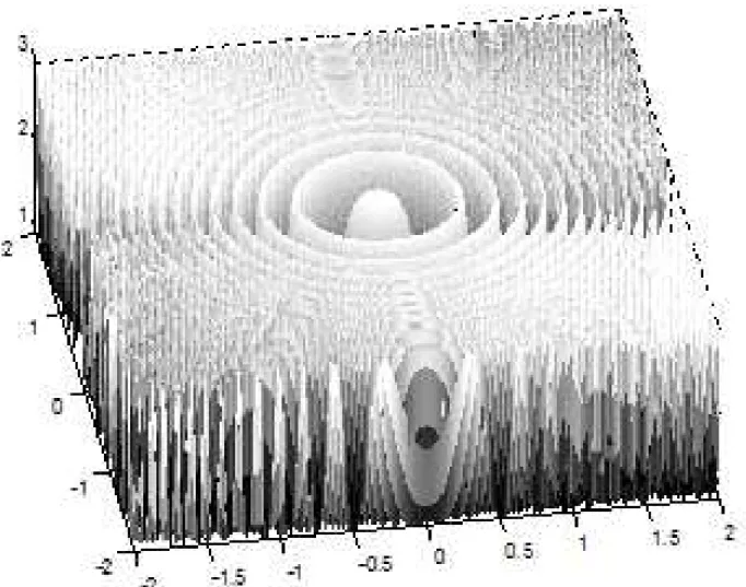
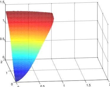
Figure 3.1 Graph of the integrand function ... 38

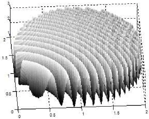
Figure 3.2 Graph of the integrand function on the constraint region ... 39

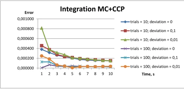
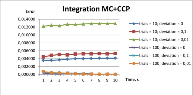
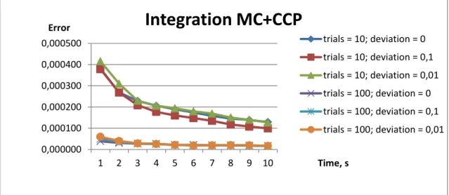
Figure 3.3 Errors of Monte Carlo integration method combined with continuous constraint programming. ... 41

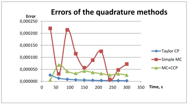
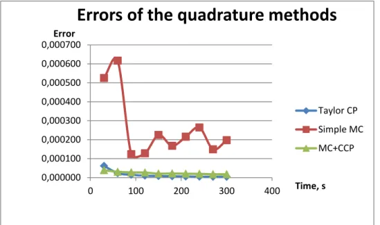
Figure 3.4 Errors of the quadrature methods... 42

Figure 3.5 Errors of Monte Carlo integration method combined with continuous constraint programming. ... 44

Figure 3.7 Graph of the integrand function ... 45

Figure 3.8 Graph of the integrand function on the constraint region ... 45

Figure 3.9 Errors of Monte Carlo integration method combined with continuous constraint programming ... 46

Figure 4.1 Mobile robot ServRobot ... 52

Figure 4.2 Extended Kalman Filter applied to the on-line SLAM problem. ... 56

Figure 4.3 Monte Carlo Localization ... 57

Figure 4.4 Robot pose on the global coordinate system ... 60

Figure 4.5 Robot pose and measurements. ... 65

(14)

xiv

Figure 4.7 Simulation results. Reduced space ... 68

Figure 4.8 Simulation results. Probability distribution ... 69

Figure 4.9 Simulation example 1. Constraint reasoning with Monte Carlo. ... 69

(15)

xv

List of Tables

Table 3.1 Integral . Relative errors ... 39

(16)

(17)

xvii

List of Algorithms

Algorithm 3.1 Branch-and-prune ... 29

Algorithm 3.2 Branch-and-prune with quadrature ... 31

Algorithm 3.3 Monte Carlo integration ... 35

Algorithm 3.4 Monte Carlo integration with deviation calculation for the interval representation ... 37

Algorithm 4.1 Computation of the probability distribution... 61

Algorithm 4.2 Monte Carlo integration for probability calculation ... 62

Algorithm 4.3 Value of probability density function calculation ... 63

Algorithm 4.4 Distance from robot to the closest object ... 64

(18)

(19)

xix

Acronyms

CCP - Continuous Constraint Programming

CCSP - Continuous Constraint Satisfaction Problem

CSP – Constraint Satisfaction Problem

CP – Constraint Programming

CPA – Constraint Propagation Algorithm

DC - Direct Current

LADAR - LAser Detection And Ranging

MC – Monte Carlo

MCL - Monte Carlo Localization

MFTP – Multivariable Fuzzy Temporal Profile model

SLAM - Simultaneous Localization and Mapping Methods

p.d.f. - probability density function

(20)

(21)

1

1. Introduction

A key element in robotics is uncertainty that arises from many factors, such

as environment, sensors, models, computations and robot actuators and motors.

Probabilistic robotics is an approach for dealing with hard robotic problems

that relies on probability theory and has a number of developed algorithms and

implemented solutions that will be specified further in this dissertation. In the

case of the robot localization problem, where sensors play a major role, errors in

measurements are unavoidable and must be considered together with the

model constraints. This requires a method for uncertainty reasoning with

mathematical models involving nonlinear constraints over continuous

variables.

(22)

2

1.1 Goals

The general goal of this work is the development of an approach that

combines safe and probabilistic reasoning for dealing with the uncertainty in

nonlinear constraint models. We propose a new technique that is based on the

combination of methods from continuous constraint programming with Monte

Carlo integration techniques. We aim to overcome the scalability problem of the

pure (safe) constraint programming approach providing the means to quickly

obtain an accurate characterization of the uncertainty. We envisage to

successfully apply this technique to probabilistic robotics and, in particular, to

show its advantages with respect to the traditional approaches for the robot

localization problem.

1.2 Area

Uncertainty occurs in stochastic environments and is a subject of study in

a number of fields, including physics, economics, statistics, engineering, and

information science. In robotics uncertainty arises from many sources.

Physical worlds are unpredictable. In robotics the environment is highly

dynamic and unpredictable that leads to the high degree of uncertainty. In

some task (such as path planning) the ignorance of uncertainty is not possible.

Sensors have number of limitations that arise from the following factors.

The range and resolution of a sensor are limited by physical laws. Image

sensors cannot see through walls and, moreover numbers of the parameters

characterizing the performance are limited. Another problem is noise, which

disturbs the measurements of the sensors. The noise in unpredictable and it

limits the information that can be extracted from sensors measurements [1].

Robot actuation involves motors that could be subject to control noise.

Some of the actuators are characterized by low noise level. However others

(23)

3

All of these factors give rise to uncertainty. A probabilistic approach

considers uncertainty and uses models to abstract useful information from the

measurements. The actual sensors always give some scatter of values measured

with some accuracy. Errors always occur in the sensor measurements.

Probabilistic robotics deals with the concepts of control and perception in

the face of uncertainty, inherent to the location of the robots which are usually

in unstructured environments. The key idea is to represent the uncertainty in an

explicit way, representing information by probability distributions over all

space of possible hypotheses instead of relying only on best estimates. In this

way, the models can represent the ambiguity and the degree of confidence in a

solid mathematics, allowing them to accommodate all sources of uncertainty.

However one of the limitations of probabilistic algorithms is the

computational complexity, because the computation of the exact posterior

distributions can be unaffordable. Also those algorithms make approximations,

since robots perform continuous processes. Another problem is lower efficiency

when compared with non-probabilistic algorithms, since the best estimate but

probability densities are considered. This is an important issue because robots,

being real-time systems, limit the amount of computation that can be carried

out. Operating in a real-time requires fast time response. Many state-of-the-art

algorithms are approximate, and are not enough accurate.

In this work we propose usage of the probabilistic constraint techniques in

the context of probabilistic robotics and in particular to solve robot localization

problems. Mobile robot localization, also known as position estimation, is the

problem of determining the pose of a robot relative to a given map of the

environment. The robot pose cannot be measured directly from the sensors, but

it can be obtained from the available with consideration of the model

constraints and the underlying uncertainty. Instead of providing a single

scenario, the most probable position of the robot in the current moment, the

proposed approach is able to characterize all possible positions (consistent with

the model) and their probabilities (in accordance with the underlying

(24)

4

The continuous probabilistic constraint framework provides expressive

mathematical model that can represent the robot localization problem. The

uncertainty and nonlinearity are taken into account in the probabilistic

constraint reasoning. The hybridization constraint branch-and-prune

algorithms with of Monte Carlo integration techniques increases the efficiency

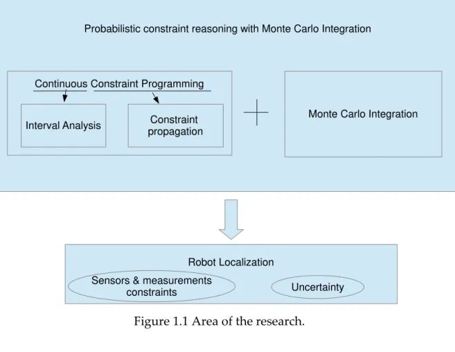
of the approach. Figure 1.1 illustrates the relevant areas of research.

Figure 1.1 Area of the research.

In continuous constraint programming the computations are supported by

interval analysis which is a set extension of numerical analysis. The

floating-point numbers are replaced by intervals that guarantee safe enclosures of the

correct values. The relations between variables are stated in the form of

constraints.

The branch-and-prune algorithms of continuous constraint programming

are aimed to cover sets of exact solutions for the constraints with sets of interval

boxes. The box is Cartesian product of intervals bounded by floating-points.

Probabilistic constraint reasoning with Monte Carlo Integration

Monte Carlo Integration Continuous Constraint Programming

Interval Analysis Constraint propagation

Robot Localization

Uncertainty Sensors & measurements

(25)

5

These algorithms recursively refine initial crude cover of the feasible space (the

set of all values, Cartesian product of the initial domains). There are two

interleaving steps - branching and pruning, which repeat until a stopping

criterion is satisfied. On the branch step the interval box is splitted into a

partition of sub-boxes (usually two). On the pruning step an interval box is

reduced from the covering into a smaller (or equal) box such that all the exact

solutions included in the original box are also included in the reduced box [2].

Continuous constraint programming provides reasoning on safe

enclosures of all consistent scenarios. Intervals are used to include all their

possible values [3]. The framework provides safe constraint propagation

techniques. Constraint propagation reduces the search space by eliminating

combinations of values that do not satisfy model constraints. However, in some

cases obtained safe enclosure of all consistent scenarios may be too extensive

and insufficient to support decisions. This can happen, if initial intervals are

wide.

The continuous probabilistic constraint framework is an extension to

constraint programming that bridges the gap between pure safe reasoning and

pure probabilistic reasoning. This framework provides the decision support in

the presence of uncertainty. The interval bounded representation of uncertainty

is complemented with a probabilistic characterization of the values

distributions. That makes possible to further characterize the scenarios with a

likelihood value.

Moreover, this approach does not suffer from the limitations of

approximation techniques, due to the constraint programming paradigm that

supports it. The approach guarantees safe bounds for the solutions and their

likelihoods.

The probabilistic constraint framework provides methods to compute

certified enclosures for the probability of consistent scenarios based on reliable

interval techniques for multidimensional quadrature. However, these methods

(26)

6

This work explores an hybrid approach that relies on constraint

programming and Monte Carlo integration to obtain estimates for the

probability of consistent scenarios. The idea is to compute close estimates of the

correct probability value by applying Monte Carlo integration techniques that

benefit from the contribution of constraint programming to reduce the sample

space into a sharp enclosure of the region of integration. Instead of computing

guaranteed results with a computationally demanding method, we aim at

obtaining accurate estimates much faster.

1.3 Contributions

This work studies the hybridization of Monte Carlo integration techniques

with continuous constraint programming for effective probabilistic constraint

reasoning. The main contributions are:

The development of an hybrid approach for probabilistic constraint reasoning that improves the efficacy of the approximate quadrature methods in

the context of the constraint programming branch-and-prune algorithm.

Implementation of the solution proposed and its benchmarking based on a set of generic experimental tests on multidimensional integrals over nonlinear

constrained boundaries.

Application of the developed techniques to the robot localization problem and analysis of its performance on a set of simulated problems.

1.4 Scheme of the document

This dissertation is structured in 5 chapters. After the first introductory

chapter the rest of the work is organized as follows:

 Chapter 2 overviews the state-of-the-art, including the basic concepts of continuous constraint programming, probability theory and quadrature

methods. Additionally it briefly summarizes the traditional applications of

(27)

7

 Chapter 3 presents our proposal to extend the constraint programming branch-and-prune algorithms with Monte Carlo integration techniques. The

probabilistic constraint reasoning is analyzed and alternative integration

approaches are suggested and evaluated on a set of experiments.

 Chapter 4 discusses the application of our approach to probabilistic robotics and, in particular to robot localization problems. The added value of

the approach is highlighted on a set of simulated problems.

(28)

(29)

9

2. State of the Art

A mathematical model is a mathematical representation of the reality,

which describes a system by a set of variables and constraints that establishes

relations between them. In engineering systems, particularly in robotics,

nonlinearity and uncertainty occur very often. Reasoning with mathematical

models under uncertainty is traditionally based on probability theory.

There are two general types of approaches for reasoning under

uncertainty. Stochastic approaches reason on the basis of the most likely

scenarios, but don't guarantee the safeness of the calculations. The drawback is

that such approaches rely on approximations and may miss relevant

satisfactory scenarios leading to erroneous decisions.

The other type of approaches provides safe enclosures of all consistent

scenarios. Continuous constraint programming operates with intervals that are

used to include all the possible values of the variables. Safe constraint pruning

techniques only eliminate combinations of values that definitely do not satisfy

the model constraints. The drawback is the consideration that all consistent

scenarios are equally likely, which can be insufficient to support decisions.

(30)

10

We believe that the combination of those two types of approaches can

provide a powerful tool for reasoning under uncertainty which may be applied

in several real-world problems, including robotic problems.

This chapter overviews the theoretical basis of continuous constraint

programming, probability constraint reasoning and Monte Carlo quadrature

methods. It also describes the real-world applications of developed methods of

those areas to robotic problems.

2.1 Continuous Constraint Programming

Constraint programming [4], [5] is a programming paradigm wherein

relations between variables are stated in the form of constraints. Mathematical

constraints are relations between variables, each ranging over a given domain.

A constraint satisfaction problem (CSP) is a classical artificial intelligence

paradigm introduced in the 1970’s. CSP is characterized by a set of variables

(each variable has associated domain of possible values), and a set of

constraints that specify relations among subsets of these variables. The

solutions of CSP are assignments of values to all variables that satisfy all the

constraints [2],[6].

Constraint programming is a form of declarative programming in the

sense that instead of specifying a sequence of steps to execute, it relies on

properties of the solutions to be found which are explicitly defined by the

constraints. The idea of constraint programming is to solve problems by stating

constraints which must be satisfied by the solutions. As such, a constraint

programming framework must provide a set of constraint-based reasoning

algorithms that take advantage of constraints to reduce the search space,

avoiding regions that are inconsistent with the constraints. These algorithms are

supported by specialized techniques that explore the specificities of the

constraint model such as the domain of its variables and the structure of its

(31)

11

Origins of continuous constraint programming comes from Davis [7],

Cleary [8] and Hyvonen [9] and later research that extended constraint

programming to continuous domains. In continuous constraint programming

the domains of the variables are real intervals and the constraints are equations

or inequalities represented by closed-form expressions (expression that can be

evaluated in a finite number of operations). In this sense the Continuous

Constraint Satisfaction Problem (CCSP) is a triple where:

 is a tuple of real variables

 is a box, the Cartesian product of intervals where each is the interval domain of variable

 is a set of numerical constraints (equations or inequalities) on subset of variables in .

Continuous constraint programming integrates techniques from constraint

programming and interval analysis into a single discipline. Interval analysis,

which addresses the use of intervals in numerical computations, is an important

component of continuous constraint programming.

2.1.1 Interval Analysis

Interval analysis was introduced in the late 1950’s [10] as a way to

represent bounds in rounding and measurement errors, and to reason with

these bounds in numerical computations. The introduction to interval analysis

can be found in [11]. In recent decades, interval analysis was widely used as the

basis for the reliable computing, calculations with guaranteed accuracy [12].

A real interval is a set of real numbers with the property that any number

that lies between two numbers in the set is also included in the set. The interval

of numbers between a and b, including a and b, is denoted [a, b] (in this work we

(32)

12

[ ] { | (2.1)

If a = b the interval is degenerated and is represented as .

The generalization of intervals to several dimensions is of major relevance

in this work. An n-dimensional box B is the Cartesian product of n intervals and

is denoted by I1× · · · × In, where each Ii is an interval.

Elementary set operations, such as ∩ (intersection), ∪ (union),  (inclusion) are valid for intervals. While the intersection between two intervals is still an

interval, this is not the case with the union of two disjoint intervals, where the

result is a set that cannot be represented exactly by a single interval. The

operation ⊎ (union hull) gives the smallest interval, containing all the elements

of both interval arguments:

[ ] ⊎ [ ] [ ] (2.2)

Interval arithmetic defines a set of operations on intervals, and is an

extension of real arithmetic for intervals. The obtained interval is the set of all

the values that result from a point-wise evaluation of the arithmetic operator on

all the values of the operands.

Let and be two real intervals. The basic interval arithmetic operators

{ are defined as:

{ | I1I2= { x  y : x I1∧ y I2 } (2.3) with  {+,−,×, /}

Under the basic interval arithmetic, the division is not defined if

.

In practice, interval arithmetic simply considers the bounds of the

operands to compute the bounds of the result, since the involved operations are

monotonic. Given two real intervals [ ] and [ ] the basic interval arithmetic

(33)

13

[ ][ ][ ] [ ] [ ] (2.4)

[ ] [ ] [ ] (2.5)

[ ] [ ] [ ] (2.6)

[ ] [ ] [ ] [ ] [ ] (2.7)

The implementation of the interval arithmetic operators is conditioned by

the floating point representation of real numbers. In order to guarantee the

correctness of the results, the above operations on the bounds of the operands

must be performed with outward rounding to the closest floating point. As

such, the computed interval is bounded by floating points and always includes

the correct real interval.

Several extensions to the basic interval arithmetic were proposed over the

years and are available in extended interval arithmetic libraries, namely:

redefinition of the division operator, allowing the denominator to contain zero;

generalization of interval arithmetic to unbounded interval arguments;

extension of the set of basic interval operators to other elementary functions

(e.g., exp, ln, power, sin, cos).

In continuous constraint programming interval arithmetic is used as a safe

method for evaluating an expression, by replacing each variable by its interval

domain, and applying recursively the interval operator evaluation rules. In fact,

the computed interval includes all possible values for the expression, but its

width may be much wider than the width of its exact range. Consequently, in

interval analysis special attention has been devoted to the definition of interval

functions that compute sharp interval images of real functions.

Moreover, interval methods are frequently used in constraint

programming due to their efficiency and reliability. One of the applications is

finding roots of equations with one variable. The combination of the Newton

method, interval analysis, and the mean value theorem gives the interval

(34)

14

the solutions of the system of non-linear equations or to prove non-existence of

solutions or.

2.1.2 Constraint Reasoning with Continuous Domains

Constraint reasoning implies the techniques for eliminating values, which

do not satisfy the constraints, from the initial search space (the Cartesian

product of all variable domains). Branch-and-prune algorithms contain

dividing and pruning steps that are recursively applied until a stopping

criterion is satisfied. The sets of values that can be proved inconsistent are

eliminated on the pruning step [3].

The safe narrowing operators (mappings between boxes) are associated

with the constraint. The operators aim to eliminate value combinations that are

incompatible with a particular constraint. These operators must satisfy the

following requirements: be correct (do not eliminate solutions) and contracting

(the obtained box is contained in the original). The properties are guaranteed

due to interval analysis methods applied.

For example, consider the constraint:

(2.8)

The following narrowing operators may be associated with this constraint

to prune the domain of each variable:

X  X  Z - Y, Y  Y  Z - X, Z  Z  X + Y (2.9)

If, for instance, the domains of the variables are X = [1,3], Y = [3,7] and

Z = [0,5] then interval arithmetic can be used to prune them to:

(35)

15

With this technique, based on interval arithmetic, safe narrowing

operators may be associated with the above constraint which are able to reduce

the original box <[1,3],[3,7],[0,5]> into <[1,2],[3,4],[4,5]> with the guarantee that

no possible solution is lost.

Once narrowing operators are associated with all the constraints of the

continuous constraint satisfaction problem, the pruning can be achieved

through constraint propagation. Narrowing operators associated with a

constraint eliminate some incompatible values from the domain of its variables

and this information is propagated to all constraints with common variables in

their scopes. The process terminates when a fixed point is reached i.e., the

domains cannot be further reduced by any narrowing operator [14].

The pruning achieved through constraint propagation is highly dependent

on the ability of the narrowing operators for discarding inconsistent value

combinations. Further pruning is usually obtained by splitting the domains and

reapplying constraint propagation to each sub-domain. In general, continuous

constraint reasoning is based on such a branch-and-prune process which will

eventually terminate due to the imposition of conditions on the branching

process (e.g. small enough domains are not considered for branching).

Since no solution is lost during the branch-and-prune process, constraint

reasoning provides a safe method for computing an enclosure of the feasible

space of a CCSP. It applies, repeatedly, branch and prune steps to reshape the

initial search space (a box) maintaining a set of working boxes (a box cover)

during the process. Moreover, some of these boxes may be classified as inner

boxes, if it can be proved that they are contained in the feasible space (again

interval analysis techniques are used to guarantee that all constraints are

satisfied).

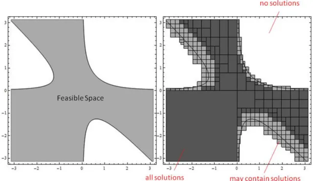
Figure 2.1 illustrates the results that can be achieved through continuous

constraint reasoning for a CCSP with two variables x and y, both ranging

(36)

16

x2_{y + xy}2 _0.5 _(2.10)

Figure 2.1 A box cover of the feasible space obtained through constraint reasoning.

As show in the figure 2.1, constraint reasoning can prove that there are

regions with no solutions (white) and find boxes where every point is a solution

(dark gray). Additionally there are some boxes that cannot be proved to contain

or not solutions (light gray). These boxes denominated boundary boxes

represent the uncertainty on the feasible space enclosure which may be reduced

by further splitting and pruning.

2.2 Probabilistic Constraint Reasoning

Probability provides a classical model for dealing with uncertainty [14].

The basic elements of probability theory are random variables, with an

associated domain, and events, which are appropriate subsets of the sample

space. A real-valued random variable is a function from the sample space into

(37)

17

A probabilistic model is an encoding of probabilistic information that

allows the probability of events to be computed, according to the axioms of

probability. In the continuous case, the usual method for specifying a

probabilistic model assumes, either explicitly or implicitly, a full joint

probability density function (p.d.f.) over the considered random variables,

which assigns a probability measure to each point of the sample space.

The probability of an event H, given a p.d.f. f, is its multidimensional

integral on the region defined by the event:

∫ (2.11)

In accordance to the axioms of probability, f must be nonnegative and

when the event is the entire sample space  then P()=1.

The idea of probabilistic constraint reasoning [3] is to associate a

probabilistic space to the classical CCSP by defining an appropriate density

function. A constraint (or set of constraints) can be viewed as an event whose

probability can be computed by integrating the density function over its

feasible space.

In general these multidimensional integrals cannot be easily computed,

since they may have no closed-form solution and the event may establish a

complex nonlinear integration boundary.

The probabilistic constraint framework relies on continuous constraint

reasoning to get a tight box cover of the region of integration and compute the

overall integral by summing up the contributions of each box in the cover.

Generic quadrature methods are used to evaluate the integral at each box.

Taylor models [15] provide certified methods to obtain sharp enclosures

for the integral at each box and are used in probabilistic constraint reasoning

[14] to compute interval enclosures for the probability of an event. To guarantee

(38)

18

differently. The inner boxes contribution to the overall integral is the interval

obtained by the certified method. However, in the case of boundary boxes, the

region is some unknown subset of the box (eventually empty) and its

contribution ranges from zero to the obtained integral over the entire box.

Although this probabilistic constraint reasoning approach outputs

guaranteed results it is computationally demanding. This justifies an hybrid

approach which relies on constraint programming to obtain a cover of the

feasible space and then uses an approximate quadrature method on this

reduced space to obtain an estimate for the probability of an event.

The study of such hybridization with approximate quadrature methods is

the subject of this work. In particular, approaches based on Monte Carlo

integration techniques are investigated.

2.3 Monte Carlo Quadrature Methods

Quadrature methods are numerical methods that aim to approximate the

value of a definite integral [16],[17]. Numerical integration is used when

integrand itself is not specified analytically; analytical representation of the

integrand is known, but it is not expressed in terms of the primitive analytic

functions; primitive function is complex.

Methods for one-dimensional integrals include [16]: Newton-Cotes

Formulas, Midpoint Rule, piecewise step function approximation, Trapezoid

Rule: piecewise linear approximation, Simpson's Rule, piecewise quadratic

approximation, Gaussian Formulas, Euler–Maclaurin formula, Romberg's

method. Methods for multidimensional integrals include: Sparse grids,

Quadrature Rules over Simplices, Monte Carlo and its modifications.

Quadrature methods based on the sparse grid approach [18],[19] consider

integration over the d-dimensional hypercube, [ ] . For spaces where

(39)

19

1963) effectively combats the curse of dimensionality. The multidimensional

quadrature formulas based on tensor products of one-dimensional formulas for

constructing sparse grids. Regardless of the size of the problem, this process

preserves the number of function evaluations and numerical within a

logarithmic factor.

Different quadrature methods were proposed for cases where the domain

is not an hypercube, but a simplex. A simplex is defined by vertices in the

n-space. The multidimensional regions of integration can often be

approximated by union of simplexes. One of the methods is the Duffy

transformation, that reduces the problem to a quadrature rule over a

hypercube.

In general, Monte Carlo methods are computational algorithms that rely

on repeated random sampling to obtain numerical results. The applications of

these methods are: integration, simulation and optimization, computational

mathematics, inverse problems.

Sampling methods, such as Monte Carlo and its modifications, contrary to

numerical quadrature rules, are more efficient for multidimensional integrals of

large dimension (d≥15). For Monte Carlo integration, the error scales like

O(1/n), where n is the number of samples, independently from the dimension of the integral. However, for substantial accuracy the convergence, a rate of

error is extremely slow. Hence, several techniques to improve the efficiency of

Monte Carlo integration were developed, including variance reduction

methods, Quasi-Monte Carlo and Adaptive Monte Carlo methods.

The Monte Carlo method is defined as following. We consider the integral

of a function f over , subset of with volume :

(40)

20

The naive approach is to sample random points on and calculate the

average value of the function. Then the integral can be approximated by:

∑ (2.13)

where n is the number of samples and is random point in .

The Monte Carlo estimate converges to the true value of the integral as

(Law of Large Numbers):

(2.14)

The error estimate for finite n is characterized by the variance of the

function :

√ (2.15)

The main advantage of Monte Carlo integration is that the error estimate

is independent of the number of dimension. The disadvantage is that integral

converges slowly to the true value as the sample size increases. There are

several approaches to improve this drawback, such as stratified sampling,

importance sampling, and control variates.

Stratified Sampling [20] is the sampling method that partition the

domain of integration into sub-domains (strata), and the overall result is

computed by summing up the results of Monte Carlo integration in each

sub-domain. This method can improve the accuracy of statistical results of Monte

Carlo method.

The integration domain Ω is partitioned into a set of m disjoint subspaces Ω1,. .. ,Ωm (strata). Then we can evaluate the integral as a sum of integrals over

(41)

21

Stratified sampling works well for low-dimensional integration, in case of

high dimensionality it does not scale well for integrals. The expected error of

this method is lower than variance of ordinary unstratified sampling.

Importance sampling [21] is another modification of Monte Carlo

method, and is used for variance reduction. Here a density function p should be

chosen similar to the integrand f. This method corresponds to a change of

integration variables

∫ ∫ (2.16)

the estimator is:

̂ ∑ (2.17)

The variance of the estimator ̂ depends on the density p(x) from which

random samples are drawn. If we choose the density p(x) intelligently, the

variance of the estimator is reduced. p(x) is called the importance density and

(2.18)

is the importance weight.

The best possible sampling density is p*(x)=c f(x) where c is the

proportionality constant:

∫ (2.19)

The constant ensures that p* is normalized:

∫ (2.20)

This gives us an estimation to the integral with zero variance, since

(42)

22

In practice, we cannot use this density, because we must know the value

of the integral we want to compute to evaluate c. However, if we choose an

importance density p(x) that has a similar shape to f(x), the variance can be

reduced. It is also important to choose an importance density p such that it is

simple and efficient to evaluate.

Importance sampling is very effective when function f(x) has large values

on small portions of the domain.

But this method has different problems and is not practical. If p goes to

zero somewhere where f is not zero, the variance can be increased and can

actually be infinite. Another common problem that happens in importance

sampling is when the sampling density has a similar shape to f(x) except that

f(x) has longer (wider) tails. In this case, the variance can become infinite.

The control variates method is a variance reduction technique. It reduce

the error of an estimate of an unknown quantity by using the information about

the errors in estimates of known quantities.

If we can rewrite the estimator as

∫ ∫ (2.22)

where integral of function is known and function has the following

property:

[ ] [ ], (2.23)

then a new estimator is

∫ ∑ (2.24)

The variance of this new estimator will be lower than the original

(43)

23

The method of control variates is more stable than importance sampling,

since zeros in g cannot induce singularities in .

Quasi-Monte Carlo methods are modifications of the Monte Carlo method

that do not require that the samples be chosen randomly. The idea is to

deterministically distribute the samples uniformly. In this methods the

irregularity of the distribution of the samples is measured and is called

discrepancy measure.

Adaptive Monte Carlo Methods introduce the idea of adaptive sampling

(or sequential sampling), to take more samples where the integrand has the

most variation. The previous taken samples are examined, and using this

information the placement of future samples is controlled. The variance of the

samples in a given domain is computed, and then more samples are taken if the

variance exceeds a given threshold.

2.4 Application of Constraint programming and Interval

Analysis to Robotics

In [5] some applications of constraint programming for robotics are

presented. The example of an application is the design of controllers for

sensory-based robots.

Many of the tools developed up to that moment in the CSP and CP

paradigms were not adequate for the task, because techniques presume an

offline model of computation, whereas controllers in real physical systems

should be designed in an online model. Furthermore, the online model must be

based on various time structures: continuous, discrete and event-based, and

computations should be performed over various type structures domains:

continuous and discrete. That requires new models of computation and

constraint programming. For this task Zhang and Mackworth [22] defined

(44)

24

asymptotically the solution set of the given constraints, possibly time-varying.

In [23], [24] robots are considered as on-line constraint-satisfying devices.

Automatic synthesis of a correct constraint-satisfying controller can be

implemented with given a constraint-based specification and a model of the

plant and the environment, that was shown for a ball-chasing robot in [25].

Later [26], [27], was designed the system to support hybrid agents i.e., agents

with both continuous and discrete interactions with their environment. A

constraint satisfying controller could be synthesized by driving the system

toward satisfying all constraints (if the robotic system deviated from a

satisfactory state it will be driven toward a satisfying state). For reactive

systems, such as controllers and signal-processing systems, timed concurrent

constraint programming was developed [28].

More recent papers in application of constraint programming in robotics

suggest different approaches. For example, in [29] in order to provide a solution

in real-time a framework was developed, that models this decision process as a

constraint satisfaction problem. It uses techniques and algorithms from

constraint programming and constraint optimization.

Using constraint programming for finding the maximal pose error

(position and rotational errors) in robotic mechanical systems is proposed in

[30]. The authors claim that their global optimizer is very competitive compared

to the other methods and provides more robust results.

Another work deals with landmark recognition in mobile robotics, using

Multivariable Fuzzy Temporal Profile model (MFTP) based on Constraint

Satisfaction Problems (CSP). This model successfully detects 95% of the

landmarks on the reference wall [31].

The application of continuous constraint programming to modular robot

control was proposed in [32]. They consider the control of modular,

(45)

25

required for typical tasks. They assumed the control problem as a constraint

problem which is a promising approach for robustly handling a variety of

non-standard constraints. A parametric model for robotic control was presented and

a generic benchmarking model for continuous constraint satisfaction problems

was proposed.

In [33] interval analysis was applied to the design and the comparison of

three-degrees-of-freedom (3-DoF) parallel kinematic machines. They introduced

an algorithm describing this method and two 3-DoF translational parallel

mechanisms designed for machining applications were compared using that

method. Also [34] considered a Gough-type parallel robot. A numerically

robust algorithm based on interval analysis was developed. It allows to solve

the forward kinematics, to determine all the possible poses of the platform for

given joint coordinates. It is possible to take into account physical and

technological constraints on the robot, such as limited motion of the passive

joints. This algorithm is competitive in terms of computation time with a

real-time algorithm such as the Newton scheme, while being safer.

Application of interval methods for certification of the kinematic

calibration of parallel robots was proposed by [35]. A certified approach for this

problem in the case of a Gough platform was developed. This approach avoids

wrong solutions produced by the classical approaches.

2.5 Summary

In this chapter the basic notions of continuous constraint programming

and interval analysis were introduced. It was discussed how probabilistic

constraint reasoning extends pure constraint reasoning with special propose

techniques for computing the probability of events defined as constraints. This

requires the computation of multidimensional integrals over constrained

nonlinear regions. Classical methods for multidimensional quadrature were

(46)

26

Finally it is shown how different methods and techniques of constraint

programming and interval analysis have been applied to robotics.

The next chapter discusses our probabilistic constraint reasoning approach

(47)

27

3. Probabilistic Reasoning with Monte Carlo

Integration

Probabilistic constraint reasoning depends on the joint cooperation of

continuous constraint programming with a multidimensional integration

method. Here the uncertainty is represented as bounded intervals with a

probabilistic characterization of the values distribution.

The probabilistic constraint framework relies on integral computations of

probabilistic density functions over constrained regions. This chapter presents

alternative approaches for the hybridization of constraint programming with

Monte Carlo integration. Continuous constraint programming is used to obtain

the feasible space, and then Monte Carlo Integration is applied on this reduced

space.

(48)

28

3.1 Probabilistic constraint reasoning

The probabilistic constraint framework complements the representation

the uncertainty by means of intervals with a probabilistic distribution of values

within such intervals. The main goal of the hybrid approach is the

development of a fast and convenient method for calculating the integral on a

bounded region. The usage of continuous constraint programming techniques

provide the results as a set of boxes that represent an enclosure of the bounded

region. Numerical and formal methods of integration can be used to compute

the value of integrals with certain accuracy. However, the error committed in

such computations can be critical for the specific problems. Whereas, certified

Taylor methods guarantee safe computations of the integral returning an

interval enclosure that contains the actual value, approximate methods aim at

obtaining fast accurate estimates.

In Chapter 2 we already introduced the notions of continuous constraint

programming and talked about the and-prune process. Several

branch-and-prune algorithms were developed, their main principle is to recursively

refine the initial interval box, which is trivially a covering of the feasible space.

The two main procedures of those algorithms are branch and prune steps which

are recursively applied until a stopping criterion is satisfied. The branching

procedure splits an interval box from the covering into a partition of sub-boxes

(usually two). The prune procedure narrows down an interval box; it either

eliminates a box from the covering or reduces it into a smaller (or equal) box

maintaining all the exact solutions. For this task a combination of constraint

propagation (CPA) and consistency techniques are usually used. A box is

reduced through the consecutive application of the consistency techniques

associated with the constraints until a fixed-point is attained [4], [6].

Algorithm 3.1 illustrates a general branch-and-prune scheme. It computes

a joint box cover from the initial domains box and is based on the algorithm

(49)

29 Branch&Prune(D, C, split, eligible, order, stop)

Input: D: initial domains box; C: set of constraints; eligible, stop: predicate; split, order: function;

Output:S: box cover;

1 { ;

2 while do

3 ;

4 ;

5 for each

6 ;

7 if

8 { ;

9 end

10 end

11 end

12 return ;

Algorithm 3.1 Branch-and-prune

The input parameters of Algorithm 3.1 are: the initial domains box D; a set

of constraints C; predicates eligible, and stop; and functions split and order. The

eligible predicate checks a box for being appropriate for further processing (for

example, it may check if it contains an interval domain that can be further

subdivided). The predicate stop imposes the stopping criterion such as

precision, cardinality of the covering, or computation time. The function split

implements the branch procedure, it defines how to partition the box into

sub-boxes. The function order defines a total order between the boxes in the cover

determining which box is retrieved for processing.

The output of Algorithm 3.1 is a box cover S for the feasible space of the

constraints in C. In order to compute it, the box cover is initialized with the

domains box (line 1) and maintained during the algorithm main cycle (lines

2-11). The first box from the current box cover that verifies the eligible predicate is

selected (boxes are ordered accordingly to the order function), and removed

from the list (line 3). Then, on the branch step, that box is split into a set of

boxes Si (line 4). Next is the prune step (lines 5-10), where each box in Si is

(50)

30

discarded (line 7), is added to the box cover (line 8). The algorithm stops when

the stopping criterion is fulfilled (line 2).

Branch-and-prune algorithms can be applied for solving different

problems. In this work we are focused on the quadrature problem, i.e.

evaluation of the multidimensional integrals. Considering this problem,

Algorithm 3.1 can be modified in order to compute the value of the integrals.

The basic idea is to calculate the value of integral on each box obtained during

the branch-and-prune algorithm. The integration can be implemented using

any method, for example using Taylor models or Monte Carlo Integration. In

this work, we compare the integration using the Taylor method, which produce

accurate results and alternatives based on Monte Carlo integration techniques

which provide approximate results. This idea is presented by Algorithm 3.2.

Basically, it is a modification of Algorithm 3.1, in which the value of the integral

on each box is computed at each step. The result of each integration is

represented as an interval, the width of which, proportional to the uncertainty

around the correct value, will be used as a selection criterion for the next box to

process.

Branch&Prune Quadrature(D, C, split, eligible, order, stop)

Input: D: initial domains box; C: set of constraints; eligible, stop: predicate; split, order: function;

Output:Q: interval;

1 ;

2 {

3 ;

4 while do

5 ;

6 ;

7 ;

8 for each

9 ;

10 if

11 ;

12 ;

(51)

31

14 end

15 end

16 end

17 return

Algorithm 3.2 Branch-and-prune with quadrature

The input parameters of the Algorithm 3.2 are similar to the previous

algorithm: the initial domains box D, the set of constraints C, predicates eligible

and stop, and functions split and order. As in the previous case, the eligible

predicate checks a box for being appropriate for further processing, the

predicate stop imposes the stopping criterion (such as precision). The function

split implements the branch procedure and the function order defines which box

is retrieved next for processing.

The first step of the algorithm is the integration of the entire domains box

considering the constraints (line 1). The integration, represented in the

pseudo code by function integrate, can be implemented by any method, such as

Taylor, Monte Carlo or any other method. In our approach we assume that the

result of the integrate function is always an interval. If the function is

implemented with the Taylor Model method then this interval must contain the

correct value. This is not the case when the Monte Carlo approach is used,

where the center or the interval is the estimated approximate value and the

width of the interval is made proportional to the estimated deviation.

During the execution of Algorithm 3.2 a box cover S is maintained where

the interval computed by function integrate is kept associated with the

respective box. At beginning the box cover is initialized with the box domains

together with the computed interval (line 2). Then, the interval is assigned to

variable (line 3) that is maintained during the processing to represent the

overall integral resulting from the contributions of every box in the cover.

The function order selects the first box from the current box cover that

(52)

32

order of boxes is determined by the width of the corresponding intervals.

Ordering them by descending interval width we aim at choosing first the boxes

with largest uncertainty on the computed integral.

The contribution of box to the overall integral must be removed from

(line 6) because we will replace such contribution by the contributions of its

sub-boxes. Notice that and are intervals and so the correct way to remove

the contribution of from is to use the special interval operator \ that reverse

the effect of the interval operator + and is defined as:

[ ] [ ] [ ] (3.1)

Afterwards, the box is splitted into sub-boxes on the branch step (line

7). On the prune step the constraint propagation algorithm is applied for

each of the boxes (lines 8-9) in order to reduce or eliminate them. If the

sub-box is not discarded (line 10), the integral value is computed over this sub-sub-box

considering the constraints (line 11). The integral value represented as an

interval is added to the previous according to the rules of interval arithmetic

(line 12). Finally the sub-box with its integral value is added to (line 13).

Basically, the integral is computed for each sub-box and the obtained

values of the integral over these sub-boxes are added (line 12) according to the

addition rule of interval analysis discussed in the Chapter 2. The widths of

those intervals serve as a criterion for choosing the box on line 5. The sum of all

those intervals is the final value of the integral.

Function can be implemented with any quadrature method. The

first method proposed in the original probabilistic constraint framework [14] is

a certified quadrature method based on Taylor models which is briefly

discussed next. Approximate implementations based on Monte Carlo

(53)

33

Taylor Models

Taylor models can be used for the computation of the quadrature over a

box. Taylor models provide efficient methods to compute enclosures for the

quadrature of multivariate functions.

A Taylor model of inside an n-dimensional box is a pair

, where is a polynomial and is an interval satisfying

The degree of the Taylor model is the degree of p.

A Taylor model of a function can be obtained from its multivariate Taylor

expansion, using the interval evaluation of the highest order derivatives to

compute rigorous bounds for the remainder [6].

Given a Taylor model of a function inside an n

-dimensional box B:

∫ ∫ (3.2)

The enclosure provided can be very sharp: if a Taylor model of order is

used, the quadrature computation has an order of convergence of . To

compute an integral of a function over some region defined as a box, the

method can be applied to obtain a sharp enclosure. However, when the region

is some unknown subset of the box (eventually empty) the integral ranges from

zero to the integral of the function maximum (minimum) over the entire box. In

this case, a sharp (and more costly) enclosure is no longer worth computing and

a cruder enclosure can be used.

3.2 Methods and algorithms of Monte Carlo integration

The Monte Carlo integration method was discussed in Chapter 2. It

(54)

34

Let consider the region with a possible nonlinear boundary,

indicator function { , an n-dimensional box and function

. Consider random sample points { uniformly distributed inside , then the approximation of the integral value is following:

∫ ∑ _(3.3)

The indicator function assumes the value 1 if the sample point

satisfy the constraints and value 0 if not.

Monte Carlo integration provides an estimate of the uncertainty in the

approximation ̂ obtained by the method. From the central limit theorem the

standard deviation of the estimate of the integral is:

√∑ ∑ ⁄ (3.4)

Thus we can represent the obtained value of the integral as the interval

[ ̂ ̂ ]. The sequence of steps for computing the interval will be the following:

1) Select random points;

2) Calculate for these points and the square of this value

; (3.5)

3) Estimate the mean of using the average of these samples:

̅ ∑ _; _(3.6)

4) Multiply with the volume to get an approximation of the integral:

̂ ∑ _; _(3.7)

5) Calculate deviation:

√∑ ∑ ⁄ ; (3.8)

6) Calculate interval:

(55)

35

The error of the estimation decreases as √ . The advantage of Monte

Carlo integration is that this result does not depend on the number of

dimensions of the integral, while most deterministic methods depend

exponentially on the dimension. The Algorithm 3.3 describes the simple Monte

Carlo integration method.

Algorithm 3.3. simpleMonteCarlo Integrate(B, C, N, f, randomGenerator, indicator,

volume)

Input: : n-dimensional box; C: set of constraints; : number of samples; , randomGenerator, indicator, volume: function;

Output:I : interval;

1 ̂ ;

2 ;

3 ;

4 while do

5

6

7 ̂ ̂

8

9 ;

10 end

11 ̂ ̂

12 √ ̂

13 [ ̂ ̂ ]

14 return

Algorithm 3.3 Monte Carlo integration

The input parameters are the n-dimensional box, the set of constraints, the

number of samples, the integrand function f, and such functions as,

randomGenerator that generates a random point within a box, indicator that

define whether a point satisfy the constraints, and volume that calculates the

volume of a box. The output is the integral, represented as an interval.

The algorithm works for a fixed number of samples (line 4) and

Probabilistic constraint reasoning with Monte Carlo integration to Robot Localization

Olga Meshcheryakova

Mestrado em Engenharia Electrotécnica,

Sistemas e Computadores

Probabilistic constraint reasoning

with Monte Carlo integration

to Robot Localization

Acknowledgements

Resumo

Abstract

Contents

List of Figures

List of Tables

List of Algorithms

Acronyms

1.

Introduction

1.1

Goals

1.2

Area

1.3

Contributions

1.4

Scheme of the document

2.

State of the Art

2.1

Continuous Constraint Programming

2.2

Probabilistic Constraint Reasoning

2.3

Monte Carlo Quadrature Methods

2.4

Application of Constraint programming and Interval

Analysis to Robotics

2.5

Summary

3.

Probabilistic Reasoning with Monte Carlo

Integration

3.2

Methods and algorithms of Monte Carlo integration