Vasco Miguel Graça Lopes
Licenciado em Engenharia InformáticaSeeded Region Growing Methods for Automatic
Upwelling Detection from Sea Surface
Temperature Images
Dissertação para obtenção do Grau de Mestre em
Engenharia Informática
Orientadora: Susana Nascimento, Profª. Auxiliar, Faculdade de Ciên-cias e Tecnologia
da Universidade Nova de Lisboa
Júri
Presidente: Doutor Pedro Abílio Duarte de Medeiros Arguente: Doutor Victor José de Almeida e Sousa Lobo
Seeded Region Growing Methods for Automatic Upwelling Detection from Sea Surface Temperature Images
Copyright © Vasco Miguel Graça Lopes, Faculdade de Ciências e Tecnologia, Universidade NOVA de LisboaA Faculdade de Ciências e Tecnologia e a Universidade NOVA de Lisboa têm o direito, perpétuo e sem limites geográficos, de arquivar e publicar esta dissertação através de exemplares impressos reproduzidos em papel ou de forma digital, ou por qualquer outro meio conhecido ou que venha a ser inventado, e de a divulgar através de repositórios científicos e de admitir a sua cópia e distribuição com objetivos educacionais ou de investigação, não comerciais, desde que seja dado crédito ao autor e editor.
Este documento foi gerado utilizando o processador (pdf)LATEX, com base no template “unlthesis” [1] desenvolvido no Dep.
A c k n o w l e d g e m e n t s
Agradeço à orientadora, Profª. Susana Nascimento, pelo acompanhamento que prestou ao longo de todo o trabalho desta dissertação e pelo rigor que foi exigido em todas as etapas.
Agradeço também o auxílio que foi prestado pelo Prof. Boris Mirkin para encontrar soluções de controlo de explosões na segmentação de imagens das Canárias, e ao Sérgio Casca pela assistência que foi dada na implementação do algoritmo SEC.
Ao Instituto de Oceanografia da Universidade de Lisboa pela cedência das imagens de Portugal, bem como aos Professores Paulo Relvas e Joaquim Luís da Faculdade de Ciências e Tecnologia da Universidade do Algarve, pela preparação e cedência das imagens das Canárias.
Também quero referir o papel importante que os professores do Departamento de Informática da FCT-UNL tiveram no meu desenvolvimento ao longo do curso.
A b s t r a c t
Coastal upwelling is a phenomenon of ocean dynamics which the Oceanographers are very interested in detect and delimitate. However, it is a tedious work to manually extract the boundaries of the upwelling area, so automatic recognition is necessary. Recently it has been proposed a new algorithm for automatic upwelling detection and delineation of its fronts, the One Seed Expanding Clustering (SEC) (Nascimento et al. (2015)). The novel features of this algorithm, compared to Seeded Region Growing (SRG) methods, include a novel homogeneity criterion in the format of a product rather than the conventional difference between a pixel value and the mean of the values over the region of interest and, the automatic threshold of the homogeneity criterion which is mathematically derived from the criterion, used in the self-tuning version of the method.
The main goal of this dissertation was to advance in the development of this algorithm in the following aspects: to make a comparative study between distinct automatic thresh-olding techniques and the self-tuning version of the SEC algorithm, and also one between the SEC and several SRG algorithms selected from the literature. It was developed an iterative version of the SEC algorithm which allowed to correctly and automatically rec-ognize discontinuous upwelling areas. The experimental results were analyzed using supervised evaluation measures, for images with ground-truth map, and unsupervised measures for images without ground-truth.
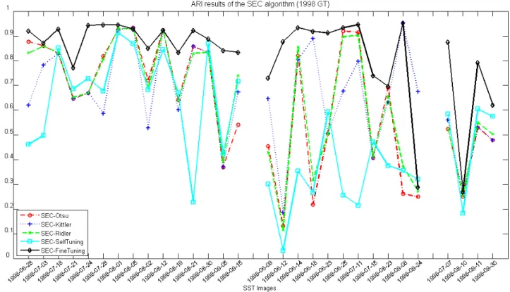
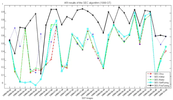
For the images with ground-truth map the SEC-SelfTuning achieved good results (F-measure≥0.7) in 62.3% of the images, the SEC-Kittler was the most reliable of the SEC versions with 78.7% positive evaluations and, the method of Adams and Bischof (1994) was best of the SRG methods with 83.6% good scores, but with manual seed selection. For images without ground-truth, the mean rate of positive classifications, using the selected evaluation measures, was 69.7% for the SEC-SelfTuning, 72.4% for the best SEC version, SEC-Ridler, and 89.5% for the Adams and Bischof (1994) method.
R e s u m o
Afloramento costeiro é um fenómeno relacionado com a dinâmica dos oceanos que os oceanógrafos estão muito interessados em detectar e delimitar. No entanto, é um tra-balho repetitivo e aborrecido de fazer, de modo que é necessário um sistema automático. Recentemente, foi proposto um novo algoritmo para a detecção automática de aflora-mento e delimitação das suas frentes, oOne Seed Expanding Clustering(SEC) (Nascimento et al. (2015)). As novas características deste algoritmo, em comparação com os métodos
Seeded Region Growing(SRG), incluem um novo critério de homogeneidade, no formato de um produto, em vez da habitual diferença entre um valor de um pixel e a média dos va-lores dentro da região de interesse e também, othresholddo critério de homogeneidade é derivado matematicamente deste critério, e é utilizado na versão auto-afinada do método.
O objetivo principal desta dissertação foi avançar no desenvolvimento deste algoritmo nos seguintes aspectos: fazer um estudo comparativo entre diversas técnicas de threshol-ding automático e a versão auto-afinada do algoritmo SEC, e também desenvolver um estudo entre o algoritmo SEC e vários algoritmos SRG selecionados da literatura. Foi de-senvolvida uma versão iterativa do algoritmo SEC que permitiu reconhecer correctamente e automaticamente áreas de afloramento descontínuas. Os resultados experimentais fo-ram analisados utilizando medidas de avaliação supervisionadas, em imagens com mapa deground-truth, e medidas não supervisionadas para imagens semground-truth.
Para as imagens com ground-truth, o SEC-SelfTuning alcançou bons resultados ( F-measure≥0,7) em 62,3% das imagens, oSEC-Kittlerfoi o mais fiável das versões do SEC com 78,7% avaliações positivas, o método de Adams e Bischof (1994) foi o melhor método SRG com 83,6% de boas pontuações, mas com a selecção manual de sementes. Para imagens semground-truth, a taxa média de classificações positivas, utilizando as medidas não supervisionadas seleccionadas, foi de 69,7% para o SEC-SelfTuning, 72,4% para a melhor versão do SEC, oSEC-Ridler, e 89,5 % para o método de Adams e Bischof (1994).
C o n t e n t s
List of Figures x
List of Tables xxii
1 Introduction 1
1.1 Motivation . . . 1
1.2 Description and Context . . . 3
1.3 Main Contributions . . . 6
1.4 Document Organization . . . 6
2 Related Work 7 2.1 Introduction to Image Segmentation . . . 7
2.2 Seeded Region Growing (SRG) . . . 8
2.2.1 Overview of SRG methods . . . 9
2.2.2 Domains of Applications . . . 15
2.2.3 Selected SRG Methods for Sea Surface Temperature (SST) Image Analysis . . . 17
2.3 Automatic Thresholding Techniques . . . 22
2.3.1 Ridler and Calvard’s method . . . 24
2.3.2 Otsu’s method . . . 24
2.3.3 Kittler and Illingworth’s method . . . 24
2.4 Evaluation Measures for Image Segmentation . . . 25
2.4.1 Supervised Evaluation Measures . . . 25
2.4.2 Unsupervised Evaluation Measures . . . 26
3 Proposed Approach 28 3.1 The Seed Expanding Cluster (SEC) . . . 28
3.1.1 The SEC method . . . 28
3.1.2 The SEC Algorithm . . . 28
3.1.3 Self-tuning version of SEC . . . 32
3.2 Iterative Seed Expanding Cluster (I-SEC) . . . 32
3.2.1 Termination condition . . . 37
C O N T E N T S
3.3 Applying the SRG Methods to SST Image Analysis . . . 42
3.3.1 Applying the Adams and Bischof Seeded Region Growing . . . 43
3.3.2 Applying the Verma Seeded Region Growing . . . 43
3.3.3 Applying the Shih and Cheng Seeded Region Growing . . . 44
3.3.4 Applying the Gambotto Seeded Region Growing . . . 45
3.3.5 Applying the Zanaty and Asaad Seeded Region Growing . . . 45
4 Experimental Study 46 4.1 Goals of the Study . . . 46
4.2 Imagery Data . . . 47
4.3 Setting of the Experiments . . . 49
4.4 Supervised Analysis of SEC versions . . . 51
4.4.1 SEC Automatic thresholding vs Self-tuning . . . 51
4.4.2 SEC versions vs other SRG Methods . . . 59
4.4.3 Study for SST Images of Canary . . . 64
4.5 Unsupervised Analysis of SEC versions . . . 71
4.5.1 Comparing the Unsupervised Evaluation Measures . . . 71
4.5.2 SEC Automatic thresholding vs Self-tuning . . . 75
4.5.3 SEC versions vs other SRG Methods . . . 76
4.6 Tuning the Density Threshold of the SEC Algorithm . . . 79
4.7 Outlook of the Results . . . 79
5 Conclusion and Future Work 82 Bibliography 84 A Analysis of Experimental Results 90 A.1 Discontinuity in the Upwelling Region . . . 90
A.2 Validation of SRG methods . . . 92
A.2.1 Validation of SRG methods with the F-measure . . . 92
A.2.2 Validation of SRG methods with ARI index . . . 99
A.2.3 Validation of SRG methods with unsupervised evaluation measures 101 A.3 Thresholds of the Unsupervised Evaluation Measures . . . 111
A.4 Empirical Study of Density Threshold . . . 112
A.5 Iterative Procedure Segmentation Study . . . 113
A.5.1 Iterative Procedure for the SEC-Otsu . . . 113
A.5.2 Iterative Procedure for the SEC-Kittler . . . 116
A.5.3 Iterative Procedure for the SEC-Ridler . . . 118
A.5.4 Iterative Procedure for the SEC-SelfTuning . . . 120
A.5.5 Iterative Procedure for the OtsuVermaSRG . . . 123
A.5.6 Iterative Procedure for the MeanVermaSRG . . . 126
C O N T E N T S
A.5.8 Iterative Procedure for the GambottoSRG . . . 130
A.5.9 Iterative Procedure for the ZanatySRG . . . 133
B Segmentation Results 135 B.1 SST Images with GT / Strong Gradients from 1998 . . . 135
B.2 SST Images with GT / Weak Gradients from 1998 . . . 141
B.3 SST Images with GT / Noisy from 1998 . . . 151
B.4 SST Images with GT from 1999 . . . 155
B.5 SST Images without ground-truth (NGT) from 1998 . . . 159
B.6 SST Images NGT from 2000 . . . 161
B.7 SST Images NGT from 2001 . . . 163
B.8 SST Images NGT from 2002 . . . 165
L i s t o f F i g u r e s
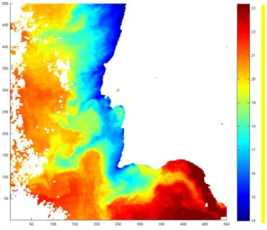
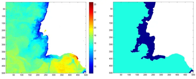
1.1 SST image of the portuguese coast (1 August 1998). The temperature values are codified in a color scale, where blue represents colder waters and red warmer waters. The white pixels represent land in the continental area, or noise derived from clouds or transmission errors from the satellite in the ocean
area. . . 2
3.1 SST image of the portuguese coast (12 June 1998). At least two relatively large, not contiguous, upwelling areas can be distinguished in this image, one in the north and other in the south, which are separated by warmer waters in the middle of the image. . . 32
3.2 1998-08-05 SEC-SelfTuning . . . 37
3.3 1998-08-05 ground-truth map . . . 37
3.4 1998-09-24 SEC-Kittler . . . 37
3.5 1998-09-24 ground-truth map . . . 37
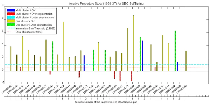
3.6 The plot shows the percentage for each termination possibility of the iterative procedure, organized by sets of images, in this case for the results of the SEC-SelfTuning. . . 38
3.7 Data related to the iterative procedure applied to the SEC-SelfTuning for the SST images of 1998 with ground-truth. The graphic which includes the values for the difference between the mean of the first region and the minimum of one relevant cluster, the relevant cluster has different meanings depending of which category described in the legend. It also includes, for each SST image, the number of the iteration that the last region of upwelling was extracted and the reason why the iterative procedure ended. . . 41
3.8 Data related to the iterative procedure applied to the SEC-SelfTuning for the SST images of 1999 with ground-truth. . . 42
4.1 Two SST images of Portugal, the one in the left was captured in 2 August 1998 and the one in the right in 28 July 1998. . . 48
L i s t o f F i g u r e s
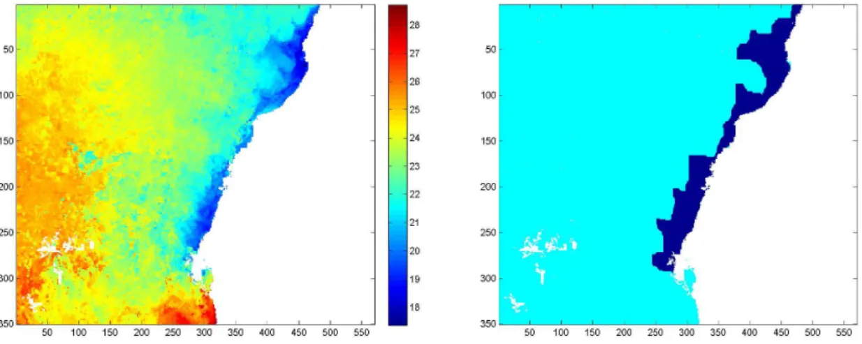
4.3 SST Image from the Canary, namedimg_58, in the left, and the correspondent ground-truth in the right. . . 49 4.4 F-measure results for the comparative study between the SEC algorithm
ver-sions. The segmentation results are from the SST images of the portuguese coast from the year 1998, which was divided into subsets of images with strong gradients in the frontier of the upwelling area, weak gradients and images with noise, from left to right in the graphic correspondingly. . . 53 4.5 Similarity thresholds that were calculated for each of the SEC algorithm
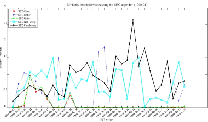
ver-sions. Higher thresholds will contain more the growth of the clusters than smaller ones. The segmentation results are from the SST images of the por-tuguese coast from the year 1998, which was divided into subsets of images with strong gradients in the frontier of the upwelling area, weak gradients and images with noise, from left to right in the graphic correspondingly. . . 54 4.6 F-measure results for the comparative study between the SEC algorithm
ver-sions. The segmentation results are from the SST images of the portuguese coast from the year 1999. . . 55 4.7 Similarity thresholds that were calculated for each of the SEC algorithm
ver-sions. Higher thresholds will contain more the growth of the clusters than smaller ones. The segmentation results are from the SST images of the por-tuguese coast from the year 1999. . . 56 4.8 The graphic shows the improvements that the fine-tuning of the density
thresh-old can have in the F-measure score. It is compared the Otsu and SEC-SelfTuning versions with their own versions, but with the fine-tuning of the density threshold. The segmentation results are from the SST images of the portuguese coast from the year 1998, which was divided into subsets of images with strong gradients in the frontier of the upwelling area, weak gradients and images with noise, from left to right in the graphic correspondingly. . . 57 4.9 The graphic shows the improvements that the fine-tuning of the density
thresh-old can have in the F-measure score. It is compared the Otsu and SEC-SelfTuning versions with their own versions, but with the fine-tuning of the density threshold. The segmentation results are from the SST images of the portuguese coast from the year 1999. . . 58 4.10 SST Image from 18 of June 1998, in the left, and the correspondent
ground-truth map in the right. . . 59 4.11 SST Image from 18 of June 1998, in the left without the fine-tuning of the
L i s t o f F i g u r e s
4.12 F-measure results for each of the SRG methods visualized in a box plot, making it possible to understand the variation of the results in the set of SST images from 1998. The box represents 50% of the data and its lower and upper lines are at the 25% and 75% quantile of the data. The remaining results are inside the vertical lines, with exception for the outliers that are represented by the plus symbols. . . 63 4.13 F-measure results for each of the SRG methods visualized in a box plot, making
it possible to understand the variation of the results in the set of SST images from 1999. . . 64 4.14 F-measure results for the comparative study between the SEC algorithm
ver-sions. The segmentation results are from the SST images of the Canary. . . . 66 4.15 Similarity thresholds that were calculated for each of the SEC algorithm
ver-sions. Higher thresholds will contain more the growth of the clusters than smaller ones. The segmentation results are from the SST images of the Canary. 67 4.16 The graphic shows the improvements that the fine-tuning of the density
thresh-old can have in the F-measure score. It is compared the Otsu and SEC-SelfTuning versions with their own versions, but with the fine-tuning of the density threshold. The segmentation results are from the SST images of the Canary. . . 68 4.17 F-measure results for each of the SRG methods visualized in a box plot, making
it possible to understand the variation of the results in the set of SST images of the Canary. . . 71 4.18 Correlation factors between the F-measure and the unsupervised evaluation
measures, for each of the versions of the SEC algorithm. It is important to have into consideration which methods should have positive and negative correlation values. . . 73 4.19 Correlation factors between the F-measure and the unsupervised evaluation
measures, for each of the SRG methods. It is important to have into consider-ation which methods should have positive and negative correlconsider-ation values. . 73
A.1 SST Image from 29 of July 1999, in the left, and the correspondent ground-truth in the right. It is an example of how noise, in this case clouds, can interfere and make necessary to the region growing algorithms to extract more than one cluster for just one continuous upwelling area. In this case, there are only one upwelling region, but the algorithm must extract two continuous regions. . . 91 A.2 SST Image from 21 of July 1999, in the left, and the correspondent
L i s t o f F i g u r e s
A.3 ARI results for the comparative study between the SEC algorithm versions. The segmentation results are from the SST images of the portuguese coast from the year 1998, which was divided into subsets of images with strong gradients in the frontier of the upwelling area, weak gradients and images with noise, from left to right in the graphic correspondingly. . . 99 A.4 ARI results for the comparative study between the SEC algorithm versions.
The segmentation results are from the SST images of the portuguese coast from the year 1999. . . 100 A.5 ARI results for the comparative study between the SEC algorithm versions.
The segmentation results are from the SST images of the Canary. . . 100 A.6 Inter-Otsu results for each of the SRG methods visualized in a box plot, making
it possible to understand the variation of the results in the set of SST images from 1998 with no ground-truth map. . . 101 A.7 Inter-Otsu results for each of the SRG methods visualized in a box plot, making
it possible to understand the variation of the results in the set of SST images from 2000 with no ground-truth map. . . 101 A.8 Inter-Otsu results for each of the SRG methods visualized in a box plot, making
it possible to understand the variation of the results in the set of SST images from 2001 with no ground-truth map. . . 102 A.9 Inter-Otsu results for each of the SRG methods visualized in a box plot, making
it possible to understand the variation of the results in the set of SST images from 2002 with no ground-truth map. . . 102 A.10 Inter-FRC results for each of the SRG methods visualized in a box plot, making
it possible to understand the variation of the results in the set of SST images from 1998 with no ground-truth map. . . 103 A.11 Inter-FRC results for each of the SRG methods visualized in a box plot, making
it possible to understand the variation of the results in the set of SST images from 2000 with no ground-truth map. . . 103 A.12 Inter-FRC results for each of the SRG methods visualized in a box plot, making
it possible to understand the variation of the results in the set of SST images from 2001 with no ground-truth map. . . 104 A.13 Inter-FRC results for each of the SRG methods visualized in a box plot, making
it possible to understand the variation of the results in the set of SST images from 2002 with no ground-truth map. . . 104 A.14 Intra-FRC results for each of the SRG methods visualized in a box plot, making
it possible to understand the variation of the results in the set of SST images from 1998 with no ground-truth map. . . 105 A.15 Intra-FRC results for each of the SRG methods visualized in a box plot, making
L i s t o f F i g u r e s
A.16 Intra-FRC results for each of the SRG methods visualized in a box plot, making it possible to understand the variation of the results in the set of SST images from 2001 with no ground-truth map. . . 106 A.17 Intra-FRC results for each of the SRG methods visualized in a box plot, making
it possible to understand the variation of the results in the set of SST images from 2002 with no ground-truth map. . . 106 A.18 CalinskiHarabasz results for each of the SRG methods in a box plot, making
it possible to understand the variation of the results in the set of SST images from 1998 with no ground-truth map. . . 107 A.19 CalinskiHarabasz results for each of the SRG methods in a box plot, making
it possible to understand the variation of the results in the set of SST images from 2000 with no ground-truth map. . . 107 A.20 CalinskiHarabasz results for each of the SRG methods in a box plot, making
it possible to understand the variation of the results in the set of SST images from 2001 with no ground-truth map. . . 108 A.21 CalinskiHarabasz results for each of the SRG methods in a box plot, making
it possible to understand the variation of the results in the set of SST images from 2002 with no ground-truth map. . . 108 A.22 Differences between the best density threshold and the empirically selected
thresholds for the SEC-SelfTuning in 1998 images. Lower differences are best. 112 A.23 Differences between the empirically selected thresholds and 0.0204 for the
SEC-SelfTuning in 1998 images. Higher differences are best. . . . 112 A.24 Data related to the iterative procedure applied to the SEC-Otsu for the SST
images from 1998 with ground-truth. . . 113 A.25 Data related to the iterative procedure applied to the SEC-Otsu for the SST
images from 1999 with ground-truth. . . 114 A.26 Data related to the iterative procedure applied to the SEC-Otsu for the SST
images of the Canary with ground-truth. . . 114 A.27 The plot shows the percentage for each termination possibility of the iterative
procedure, organized by sets of images, in this case for the results of the SEC-Otsu. . . 115 A.28 Data related to the iterative procedure applied to the SEC-Kittler for the SST
images from 1998 with ground-truth. . . 116 A.29 Data related to the iterative procedure applied to the SEC-Kittler for the SST
images from 1999 with ground-truth. . . 116 A.30 Data related to the iterative procedure applied to the SEC-Kittler for the SST
images of the Canary with ground-truth. . . 117 A.31 The plot shows the percentage for each termination possibility of the iterative
L i s t o f F i g u r e s
A.32 Data related to the iterative procedure applied to the SEC-Ridler for the SST images from 1998 with ground-truth. . . 118 A.33 Data related to the iterative procedure applied to the SEC-Ridler for the SST
images from 1999 with ground-truth. . . 118 A.34 Data related to the iterative procedure applied to the SEC-Ridler for the SST
images of the Canary with ground-truth. . . 119 A.35 The plot shows the percentage for each termination possibility of the iterative
procedure, organized by sets of images, in this case for the results of the SEC-Ridler. . . 119 A.36 Data related to the iterative procedure applied to the SEC-SelfTuning for the
SST images from 1998 with ground-truth. . . 120 A.37 Data related to the iterative procedure applied to the SEC-SelfTuning for the
SST images from 1999 with ground-truth. . . 120 A.38 Data related to the iterative procedure applied to the SEC-SelfTuning for the
SST images of the Canary with ground-truth. . . 121 A.39 The plot shows the percentage for each termination possibility of the iterative
procedure, organized by sets of images, in this case for the results of the SEC-SelfTuning. . . 122 A.40 Data related to the iterative procedure applied to the OtsuVermaSRG for the
SST images from 1998 with ground-truth. . . 123 A.41 Data related to the iterative procedure applied to the OtsuVermaSRG for the
SST images from 1999 with ground-truth. . . 123 A.42 Data related to the iterative procedure applied to the OtsuVermaSRG for the
SST images of the Canary with ground-truth. . . 124 A.43 The plot shows the percentage for each termination possibility of the
itera-tive procedure, organized by sets of images, in this case for the results of the OtsuVermaSRG. . . 125 A.44 Data related to the iterative procedure applied to the MeanVermaSRG for the
SST images from 1998 with ground-truth. . . 126 A.45 Data related to the iterative procedure applied to the MeanVermaSRG for the
SST images from 1999 with ground-truth. . . 126 A.46 Data related to the iterative procedure applied to the MeanVermaSRG for the
SST images of the Canary with ground-truth. . . 127 A.47 The plot shows the percentage for each termination possibility of the
itera-tive procedure, organized by sets of images, in this case for the results of the MeanVermaSRG. . . 128 A.48 Data related to the iterative procedure applied to the ShihSRG for the SST
images from 1998 with ground-truth. . . 129 A.49 Data related to the iterative procedure applied to the ShihSRG for the SST
L i s t o f F i g u r e s
A.50 Data related to the iterative procedure applied to the ShihSRG for the SST
images of the Canary with ground-truth. . . 130
A.51 Data related to the iterative procedure applied to the GambottoSRG for the SST images from 1998 with ground-truth. . . 130
A.52 Data related to the iterative procedure applied to the GambottoSRG for the SST images from 1999 with ground-truth. . . 131
A.53 Data related to the iterative procedure applied to the GambottoSRG for the SST images of the Canary with ground-truth. . . 131
A.54 The plot shows the percentage for each termination possibility of the itera-tive procedure, organized by sets of images, in this case for the results of the GambottoSRG. . . 132
A.55 Data related to the iterative procedure applied to the ZanatySRG for the SST images from 1998 with ground-truth. . . 133
A.56 Data related to the iterative procedure applied to the ZanatySRG for the SST images from 1999 with ground-truth. . . 133
A.57 Data related to the iterative procedure applied to the ZanatySRG for the SST images of the Canary with ground-truth. . . 134
A.58 The plot shows the percentage for each termination possibility of the itera-tive procedure, organized by sets of images, in this case for the results of the ZanatySRG. . . 134
B.1 1998-08-02 . . . 135
B.2 1998-08-02 ground-truth map . . . 135
B.3 1998-08-02 SEC-Otsu . . . 135
B.4 1998-08-02 SEC-Kittler . . . 135
B.5 1998-08-02 SEC-Ridler . . . 136
B.6 1998-08-02 SEC-SelfTuning . . . 136
B.7 1998-08-02 AdamsSRG . . . 136
B.8 1998-08-02 OtsuVermaSRG . . . 136
B.9 1998-08-02 MeanVermaSRG . . . 136
B.10 1998-08-02 ShihSRG . . . 136
B.11 1998-08-02 GambottoSRG . . . 137
B.12 1998-08-02 ZanatySRG . . . 137
B.13 1998-08-05 . . . 137
B.14 1998-08-05 ground-truth map . . . 137
B.15 1998-08-05 SEC-Otsu . . . 137
B.16 1998-08-05 SEC-Kittler . . . 137
B.17 1998-08-05 SEC-Ridler . . . 138
B.18 1998-08-05 SEC-SelfTuning . . . 138
B.19 1998-08-05 AdamsSRG . . . 138
L i s t o f F i g u r e s
B.21 1998-08-05 MeanVermaSRG . . . 138
B.22 1998-08-05 ShihSRG . . . 138
B.23 1998-08-05 GambottoSRG . . . 139
B.24 1998-08-05 ZanatySRG . . . 139
B.25 1998-09-15 . . . 139
B.26 1998-09-15 ground-truth map . . . 139
B.27 1998-09-15 SEC-Otsu . . . 139
B.28 1998-09-15 SEC-Kittler . . . 139
B.29 1998-09-15 SEC-Ridler . . . 140
B.30 1998-09-15 SEC-SelfTuning . . . 140
B.31 1998-09-15 AdamsSRG . . . 140
B.32 1998-09-15 OtsuVermaSRG . . . 140
B.33 1998-09-15 MeanVermaSRG . . . 140
B.34 1998-09-15 ShihSRG . . . 140
B.35 1998-09-15 GambottoSRG . . . 141
B.36 1998-09-15 ZanatySRG . . . 141
B.37 1998-06-14 . . . 141
B.38 1998-06-14 ground-truth map . . . 141
B.39 1998-06-14 SEC-Otsu . . . 141
B.40 1998-06-14 SEC-Kittler . . . 141
B.41 1998-06-14 SEC-Ridler . . . 142
B.42 1998-06-14 SEC-SelfTuning . . . 142
B.43 1998-06-14 AdamsSRG . . . 142
B.44 1998-06-14 OtsuVermaSRG . . . 142
B.45 1998-06-14 MeanVermaSRG . . . 142
B.46 1998-06-14 ShihSRG . . . 142
B.47 1998-06-14 GambottoSRG . . . 143
B.48 1998-06-14 ZanatySRG . . . 143
B.49 1998-07-11 . . . 143
B.50 1998-07-11 ground-truth map . . . 143
B.51 1998-07-11 SEC-Otsu . . . 143
B.52 1998-07-11 SEC-Kittler . . . 143
B.53 1998-07-11 SEC-Ridler . . . 144
B.54 1998-07-11 SEC-SelfTuning . . . 144
B.55 1998-07-11 AdamsSRG . . . 144
B.56 1998-07-11 OtsuVermaSRG . . . 144
B.57 1998-07-11 MeanVermaSRG . . . 144
B.58 1998-07-11 ShihSRG . . . 144
B.59 1998-07-11 GambottoSRG . . . 145
B.60 1998-07-11 ZanatySRG . . . 145
L i s t o f F i g u r e s
B.62 1998-07-15 ground-truth map . . . 145
B.63 1998-07-15 SEC-Otsu . . . 145
B.64 1998-07-15 SEC-Kittler . . . 145
B.65 1998-07-15 SEC-Ridler . . . 146
B.66 1998-07-15 SEC-SelfTuning . . . 146
B.67 1998-07-15 AdamsSRG . . . 146
B.68 1998-07-15 OtsuVermaSRG . . . 146
B.69 1998-07-15 MeanVermaSRG . . . 146
B.70 1998-07-15 ShihSRG . . . 146
B.71 1998-07-15 GambottoSRG . . . 147
B.72 1998-07-15 ZanatySRG . . . 147
B.73 1998-08-23 . . . 147
B.74 1998-08-23 ground-truth map . . . 147
B.75 1998-08-23 SEC-Otsu . . . 147
B.76 1998-08-23 SEC-Kittler . . . 147
B.77 1998-08-23 SEC-Ridler . . . 148
B.78 1998-08-23 SEC-SelfTuning . . . 148
B.79 1998-08-23 AdamsSRG . . . 148
B.80 1998-08-23 OtsuVermaSRG . . . 148
B.81 1998-08-23 MeanVermaSRG . . . 148
B.82 1998-08-23 ShihSRG . . . 148
B.83 1998-08-23 GambottoSRG . . . 149
B.84 1998-08-23 ZanatySRG . . . 149
B.85 1998-09-08 . . . 149
B.86 1998-09-08 ground-truth map . . . 149
B.87 1998-09-08 SEC-Otsu . . . 149
B.88 1998-09-08 SEC-Kittler . . . 149
B.89 1998-09-08 SEC-Ridler . . . 150
B.90 1998-09-08 SEC-SelfTuning . . . 150
B.91 1998-09-08 AdamsSRG . . . 150
B.92 1998-09-08 OtsuVermaSRG . . . 150
B.93 1998-09-08 MeanVermaSRG . . . 150
B.94 1998-09-08 ShihSRG . . . 150
B.95 1998-09-08 GambottoSRG . . . 151
B.96 1998-09-08 ZanatySRG . . . 151
B.97 1998-07-07 . . . 151
B.98 1998-07-07 ground-truth map . . . 151
B.99 1998-07-07 SEC-Otsu . . . 151
B.1001998-07-07 SEC-Kittler . . . 151
B.1011998-07-07 SEC-Ridler . . . 152
L i s t o f F i g u r e s
B.1031998-07-07 AdamsSRG . . . 152
B.1041998-07-07 OtsuVermaSRG . . . 152
B.1051998-07-07 MeanVermaSRG . . . 152
B.1061998-07-07 ShihSRG . . . 152
B.1071998-07-07 GambottoSRG . . . 153
B.1081998-07-07 ZanatySRG . . . 153
B.1091998-09-30 . . . 153
B.1101998-09-30 ground-truth map . . . 153
B.1111998-09-30 SEC-Otsu . . . 153
B.1121998-09-30 SEC-Kittler . . . 153
B.1131998-09-30 SEC-Ridler . . . 154
B.1141998-09-30 SEC-SelfTuning . . . 154
B.1151998-09-30 AdamsSRG . . . 154
B.1161998-09-30 OtsuVermaSRG . . . 154
B.1171998-09-30 MeanVermaSRG . . . 154
B.1181998-09-30 ShihSRG . . . 154
B.1191998-09-30 GambottoSRG . . . 155
B.1201998-09-30 ZanatySRG . . . 155
B.1211999-09-01 . . . 155
B.1221999-09-01 ground-truth map . . . 155
B.1231999-09-01 SEC-Otsu . . . 155
B.1241999-09-01 SEC-Kittler . . . 155
B.1251999-09-01 SEC-Ridler . . . 156
B.1261999-09-01 SEC-SelfTuning . . . 156
B.1271999-09-01 AdamsSRG . . . 156
B.1281999-09-01 OtsuVermaSRG . . . 156
B.1291999-09-01 MeanVermaSRG . . . 156
B.1301999-09-01 ShihSRG . . . 156
B.1311999-09-01 GambottoSRG . . . 157
B.1321999-09-01 ZanatySRG . . . 157
B.1331999-09-10 . . . 157
B.1341999-09-10 ground-truth map . . . 157
B.1351999-09-10 SEC-Otsu . . . 157
B.1361999-09-10 SEC-Kittler . . . 157
B.1371999-09-10 SEC-Ridler . . . 158
B.1381999-09-10 SEC-SelfTuning . . . 158
B.1391999-09-10 AdamsSRG . . . 158
B.1401999-09-10 OtsuVermaSRG . . . 158
B.1411999-09-10 MeanVermaSRG . . . 158
B.1421999-09-10 ShihSRG . . . 158
L i s t o f F i g u r e s
B.1441999-09-10 ZanatySRG . . . 159
B.1451998-08-04 . . . 159
B.1461998-08-04 SEC-Otsu . . . 159
B.1471998-08-04 SEC-Kittler . . . 159
B.1481998-08-04 SEC-Ridler . . . 160
B.1491998-08-04 SEC-SelfTuning . . . 160
B.1501998-08-04 AdamsSRG . . . 160
B.1511998-08-04 OtsuVermaSRG . . . 160
B.1521998-08-04 MeanVermaSRG . . . 160
B.1531998-08-04 ShihSRG . . . 160
B.1541998-08-04 GambottoSRG . . . 161
B.1551998-08-04 ZanatySRG . . . 161
B.1562000-08-08 . . . 161
B.1572000-08-08 SEC-Otsu . . . 161
B.1582000-08-08 SEC-Kittler . . . 161
B.1592000-08-08 SEC-Ridler . . . 162
B.1602000-08-08 SEC-SelfTuning . . . 162
B.1612000-08-08 AdamsSRG . . . 162
B.1622000-08-08 OtsuVermaSRG . . . 162
B.1632000-08-08 MeanVermaSRG . . . 162
B.1642000-08-08 ShihSRG . . . 162
B.1652000-08-08 GambottoSRG . . . 163
B.1662000-08-08 ZanatySRG . . . 163
B.1672001-08-04 . . . 163
B.1682001-08-04 SEC-Otsu . . . 163
B.1692001-08-04 SEC-Kittler . . . 163
B.1702001-08-04 SEC-Ridler . . . 164
B.1712001-08-04 SEC-SelfTuning . . . 164
B.1722001-08-04 AdamsSRG . . . 164
B.1732001-08-04 OtsuVermaSRG . . . 164
B.1742001-08-04 MeanVermaSRG . . . 164
B.1752001-08-04 ShihSRG . . . 164
B.1762001-08-04 GambottoSRG . . . 165
B.1772001-08-04 ZanatySRG . . . 165
B.1782002-07-31 . . . 165
B.1792002-07-31 SEC-Otsu . . . 165
B.1802002-07-31 SEC-Kittler . . . 165
B.1812002-07-31 SEC-Ridler . . . 166
B.1822002-07-31 SEC-SelfTuning . . . 166
B.1832002-07-31 AdamsSRG . . . 166
L i s t o f F i g u r e s
B.1852002-07-31 MeanVermaSRG . . . 166
B.1862002-07-31 ShihSRG . . . 166
B.1872002-07-31 GambottoSRG . . . 167
B.1882002-07-31 ZanatySRG . . . 167
B.189img_262 . . . . 167
B.190img_262 ground-truth map . . . . 167
B.191img_262 SEC-Otsu . . . . 167
B.192img_262 SEC-Kittler . . . . 167
B.193img_262 SEC-Ridler . . . . 168
B.194img_262 SEC-SelfTuning . . . . 168
B.195img_262 AdamsSRG . . . . 168
B.196img_262 OtsuVermaSRG . . . . 168
B.197img_262 MeanVermaSRG . . . . 168
B.198img_262 ShihSRG . . . . 168
B.199img_262 GambottoSRG . . . . 169
B.200img_262 ZanatySRG . . . . 169
B.201img_336 . . . . 169
B.202img_336 ground-truth map . . . . 169
B.203img_336 SEC-Otsu . . . . 169
B.204img_336 SEC-Kittler . . . . 169
B.205img_336 SEC-Ridler . . . . 170
B.206img_336 SEC-SelfTuning . . . . 170
B.207img_336 AdamsSRG . . . . 170
B.208img_336 OtsuVermaSRG . . . . 170
B.209img_336 MeanVermaSRG . . . . 170
B.210img_336 ShihSRG . . . . 170
B.211img_336 GambottoSRG . . . . 171
L i s t o f Ta b l e s
1.1 Table that contains the abbreviations for the different methods that were used in the studies, divided in separated categories and with the reference to the section of the dissertation document where the correspondent method was presented. . . 5
2.1 Definitions and notation necessary to describe thresholding algorithms (Prieto et al. (2012)): . . . 24
4.1 Table that accounts for how frequent each version of the SEC algorithm, ex-cluding the fine-tuning version, had the best score when segmenting an SST image of the portuguese coast. It is also accounted the frequency that each version had F-measure scores superior or equal to 0.7, which was empirically identified has a threshold for separating good from bad segmentation results. The best versions scores are bold in the table, for each of the sets of images and information that is being analyzed. . . 52 4.2 Table that accounts for how frequent SRG method had the best score when
segmenting an SST image of the portuguese coast. . . 61 4.3 Table that accounts for how frequent each version of the SEC algorithm,
ex-cluding the fine-tuning version, had the best score when segmenting an SST image of the Canary. It is also accounted the frequency that each version had F-measure scores superior or equal to 0.7, which was empirically identified has a threshold for separating good from bad segmentation results. The best versions scores are bold in the table, for each of the sets of images and infor-mation that is being analyzed. . . 66 4.4 Table that accounts for how frequent each version of the SEC algorithm,
L i s t o f T a b l e s
4.5 Accuracy that each unsupervised evaluation measure had when applied to each SRG method. Underlined are the three most accurate evaluation mea-sures for each of the SRG methods. In the bottom line it can be seen the percentage of times that each unsupervised evaluation measure was in the three most accurate for each SRG method (Success Rate). The values in bold are the ones where the correlation to the F-measure was better, meaning higher or lower than 0.2 or -0.2, depending if for the given unsupervised evaluation measure the ideal correlation should be positive or negative correspondingly. 75 4.6 Table that accounts for how frequent each version of the SEC algorithm and
each SRG method had positive scores given by each unsupervised evaluation measures, when segmenting SST image without ground-truth. The best SRG methods scores are bold in the table. In the bottom lines it can be seen the mean rate of positive classifications given by the select four best unsupervised evaluation measures, and the correspondent standard deviation. . . 78
A.1 Images with discontinuity that need more than one iteration to extract the full upwelling area and the correspondent cause of the discontinuity. . . 92 A.2 Table with the F-measure results for the comparative study between the SEC
algorithm and the SRG methods applied to the extraction of upwelling context. The segmentation results are from the SST images of the portuguese coast from the year 1998, with strong gradients in the frontier of the upwelling area. The best scores for each SST image are highlighted in bold. . . 93 A.3 Table with the F-measure results for the comparative study between the SEC
algorithm and the SRG methods applied to the extraction of upwelling context. The segmentation results are from the SST images of the portuguese coast from the year 1998, with weak gradients in the frontier of the upwelling area. The best scores for each SST image are highlighted in bold. . . 94 A.4 Table with the F-measure results for the comparative study between the SEC
algorithm and the SRG methods applied to the extraction of upwelling context. The segmentation results are from the SST images of the portuguese coast from the year 1998, with noise interfering with the segmentation process. The best scores for each SST image are highlighted in bold. . . 95 A.5 Table with the F-measure results for the comparative study between the SEC
L i s t o f T a b l e s
A.6 Table with the F-measure results for the comparative study between the SEC algorithm and the SRG methods applied to the extraction of upwelling context. The segmentation results are from the SST images of the portuguese coast from the year 1999. The best scores for each SST image are highlighted in bold. (Part 2/2) . . . 97 A.7 Table with the F-measure results for the comparative study between the SEC
algorithm and the SRG methods applied to the extraction of upwelling context. The segmentation results are from the SST images of the Canary. The best scores for each SST image are highlighted in bold. . . 98 A.8 Table that accounts for how frequent each version of the SEC algorithm,
ex-cluding the fine-tuning version, and each SRG method had good score, rela-tively to the correspondent threshold, when segmenting SST image without ground-truth. The best SRG methods scores are bold in the table, for each of the sets of images and information that is being analyzed. (Part 1/2) . . . 109 A.9 Table that accounts for how frequent each version of the SEC algorithm,
ex-cluding the fine-tuning version, and each SRG method had good score, rela-tively to the correspondent threshold, when segmenting SST image without ground-truth. The best SRG methods scores are bold in the table, for each of the sets of images and information that is being analyzed. (Part 2/2) . . . 110 A.10 Table with the produced thresholds using the Information Gain method. For
each region growing algorithm, different thresholds were calculated for the many unsupervised evaluation measures. The values in bold text are the ones where the correlation to the F-measure was better, meaning higher or lower than 0.2 or -0.2, depending if for the given unsupervised evaluation measure the ideal correlation should be positive or negative correspondingly. . . 111 A.11 Table with the produced thresholds using the Otsu’s method. For each region
C
h
a
p
t
e
r
1
I n t r o d u c t i o n
1.1 Motivation
Coastal upwelling is an oceanographic phenomenon characterized by the presence, at the sea surface, of colder and nutrient rich waters which are driven by the wind force over the continental shelf, and by filaments of upwelled waters extended for a large area. It is expressed by alterations in the movement of surface water masses perpendicular to the coast line, which come to replace warmer waters, usually surface water with low nutrient levels. Diverse ecological effects derive from upwelling, but one impact is especially note-worthy. When upwelling brings nutrient-rich waters to the surface, it supports blooms of phytoplankton which are the energy base for large animal populations higher in the food chain, making its detection indispensable to fisheries. Delimitation of this phenomenon is also important to the development of climate models, detection of pollutants and general coastal monitoring.
C H A P T E R 1 . I N T R O D U C T I O N
Oceanographers hands, but also because of the subjectivity inherent to visual inspection, so an objective approach to extract the upwelling is necessary. Also, it is too difficult to deal with upwelling regions with transition zones characterized by smooth thermal boundaries, where it is hard to make the distinction between the objects of interest and the background.
Figure 1.1: SST image of the portuguese coast (1 August 1998). The temperature values are codified in a color scale, where blue represents colder waters and red warmer waters. The white pixels represent land in the continental area, or noise derived from clouds or transmission errors from the satellite in the ocean area.
Different approaches have been proposed in the past to do automatic upwelling de-tection from remote sensing images, like the example image in Figure 1.1, where the upwelling areas are represented by blue tones corresponding to colder waters and, the lateral yellow bar represents contains the color that codifies the temperature at the bound-ary.
C H A P T E R 1 . I N T R O D U C T I O N
of mesoscale frontal activity based on the edge detection algorithm initially presented by Cayula and Cornillon (1992); also in (Tamim et al. (2013)) for automatic detection and extraction of upwelling areas an approach is presented, based on the evaluation and comparison between two unsupervised classification methods, Otsu’s method and Fuzzy C-means. However, these approaches require, to achieve an admissible segmentation, a more or less complex pre-processing stage, with exception for the work of Tamim et al. (2013).
In (Nascimento et al. (2005)) the segmentation of SST images was successfully achieved using the fuzzy c-means algorithm, however it did not provide an automatic mechanism to make the delimitation of the frontier of upwelling areas. This problem was solved, as described in (Nascimento and Franco (2009)), by adding a step of frontier detection after the segmentation phase. Nascimento et al. (2012) developed a fully automated fuzzy clustering method to solve the problem of automatic recognition of upwelling ar-eas in SST images. The system presented, FuzzyUPWELL, provides a framework for an unsupervised segmentation and delimitation of upwelling areas. The FuzzyUPWELL system integrates an unsupervised fuzzy clustering algorithm, the Anomalous Pattern Fuzzy Clustering (AP-FCM), a threshold procedure to determine the upwelling fronts that combines a variety of features extracted from the obtained clusters, a mechanism to delimitate the upwelling areas by fuzzy boundaries defined from measures of classifi-cation uncertainty, and a Graphical User Interface (GUI). Although the FuzzyUPWELL had shown to be a reliable system, it only operates over the temperature data during the segmentation process, not taking directly into account the geographic information about the clusters it creates. Moreover, the delineation of the upwelling front is a stage separated from the segmentation process.
Therefore, in (Nascimento et al. (2015)) it was proposed a new method, the Seed Expanding Cluster algorithm (SEC) inspired on the popular Seeded Region Growing (SRG) algorithm (Adams and Bischof (1994)), and that takes into account not only the temperature value of the pixel, but also its spacial context, in order to model the process of upwelling formation as a process of combining pixels, into a progressive bigger region, according to the similarity of their temperatures to the temperature of a seed point at the beginning, which is chosen as the pixel with lower temperature. The SEC algorithm has shown promising results in its ability to automatically recognize upwelling area and its frontline from SST images.
The SEC algorithm does not require posterior steps of delimitation of the frontier of upwelling areas. In each iteration of the algorithm a new frontier to the cluster is being defined, so the final frontier contains the pixels that delimit the upwelling area.
1.2 Description and Context
C H A P T E R 1 . I N T R O D U C T I O N
Region Growing method introduced by Adams and Bischof (1994), but is a considerably modified version of it, and it belongs to the region growing family of algorithms. The SRG algorithms are characterized by growing a region whenever its interior is homogeneous according to a certain feature of interest, and the region growing begins from one initial seed or multiple seeds if the objective is to segment into multiple areas, by adding similar neighboring pixels according to a homogeneity criterion.
The SEC algorithm is conceptually similar to most of SRG methods, but it is impor-tant to salient its specifications. The algorithm starts its growing process from one seed only and adds pixels to the region using a novel homogeneity criteria, in the form of a product rather than a difference as usual in most of the approaches of SRG algorithms. Other important characteristic of this algorithm is that the threshold of the homogeneity criterion is mathematically derived from this criterion, which is a unique feature as com-pared to other adaptive thresholding SRG algorithms presented in the literature. This last characteristic is used in the Self-tuning Seeded Expanding Clustering (SEC-SelfTuning, for short) version. To control the expansion of the region, a threshold value for the ho-mogeneity criterion must be set, however it is sometimes a difficult and tedious work to the user to do, so to fully automate the SEC algorithm a self-tuning version was proposed. It is important to compare this self-tuning version with other versions of the algorithm, where automatic thresholding techniques can be used to find an adequate threshold value without user intervention. This methods to tune the threshold value are already applied in image segmentation, where the calculated threshold value is used to separate an object from the background of the image. Different thresholding methods must be tested and their effectiveness evaluated. The self-tuning version of the algorithm will be compared with other version of the algorithm where the homogeneity threshold value is estab-lished by the selected automatically thresholding methods (Ridler and Calvard (1978); Otsu (1979); Kittler and Illingworth (1986)).
An iterative version of the algorithm is also to be produced. The SEC algorithm only grows one region, however an extension of it will extract several regions of the phenomenon under study, which sometimes does not cover a contiguous area of ocean.
C H A P T E R 1 . I N T R O D U C T I O N
of images to be analyzed, have assigned to them a binary ground-truth map, delineated by expert oceanographers, representing areas of upwelling and non-upwelling. For these images, supervised techniques to evaluate image segmentation can be applied, which compare the ground-truth to the segmentation result (Zhang (1996)). However, many images can not have a reference image to evaluate the quality of the segmentation, and for fully automate the process and avoid tedious pre-processing by the experts, it is necessary to use unsupervised evaluation techniques (Zhang et al. (2008)).
Many methods are necessary to complete the proposed study, and for convenience short names were attributed for each one, and can be seen in the Table 1.1. The abbre-viated names are divided in the the categories of SEC versions, SRG methods used in the comparative study and unsupervised evaluation measures that were used to test the quality in images that did not had ground-truth map associated to them.
Table 1.1: Table that contains the abbreviations for the different methods that were used in the studies, divided in separated categories and with the reference to the section of the dissertation document where the correspondent method was presented.
Category Method Abbreviation Described In
SEC Versions
SEC-Otsu Section 3.1.1 and 2.3.2
SEC-Kittler Section 3.1.1 and 2.3.3
SEC-Ridler Section 3.1.1 and 2.3.1
SEC-SelfTuning Section 3.1.1 and 3.1.3 SEC-FineTuning Section 3.1.1 and 4.3
SRG Methods
AdamsSRG Section 2.2.3.1
OtsuVermaSRG Section 2.2.3.2
MeanVermaSRG Section 2.2.3.2
ShihSRG Section 2.2.3.3
GambottoSRG Section 2.2.3.4
ZanatySRG Section 2.2.3.5
Unsupervised Evaluation Measures
Intra_LN Section 2.4.2, Measure (i)
Inter_Otsu Section 2.4.2, Measure (vi)
Inter_FRC Section 2.4.2, Measure (iv)
Intra_FRC Section 2.4.2, Measure (iii)
Intra_Liu Section 2.4.2, Measure (ix)
C H A P T E R 1 . I N T R O D U C T I O N
1.3 Main Contributions
The main contributions of this dissertation are three-fold:
1. To make a comparative study among distinct automatic thresholding techniques (Ridler and Calvard (1978); Otsu (1979); Kittler and Illingworth (1986)) and the self-tuning version of the SEC algorithm in order to find the best thresholding method to guide the growing of the cluster;
2. To realize an extensive comparative experimental study between several SRG algo-rithms established in the literature (Adams and Bischof (1994); Gambotto (1993); Shih and Cheng (2005); Verma et al. (2011); Zanaty and Asaad (2013)) and the SEC algorithm, to study its effectiveness on the automatic upwelling detection for several years of images;
3. To develop an iterative version of the SEC algorithm that allows to recognize dis-continuous upwelling regions. This iterative version of SEC sequentially extracts clusters one by one until a pre-specified number of clusters be recognized. The iterative procedure will be used on the two previous comparative studies.
Transversal to the former contributions is the comparative evaluation of the exper-imental results. For that, several supervised and unsupervised validation indices will be applied.
1.4 Document Organization
C
h
a
p
t
e
r
2
R e l a t e d Wo r k
2.1 Introduction to Image Segmentation
The process of partitioning an image into multiple segments, with the objective of chang-ing the representation of an image into somethchang-ing meanchang-ingful and easier to analyze is called image segmentation. It is the low-level operation that targets to partitioning im-ages by determining disjoint and homogeneous regions or, equivalently, by finding edges or boundaries and, it is a first step before applying to images higher-level operations such as recognition, semantic interpretation, and representation. This was explained in Luc-cheseyz and Mitray (2001), which presented a survey on color image segmentation since most of the methods till that time were focused on segmentation of gray-level images.
There are a lot of different segmentation techniques present in the literature (Haral-ick (1983); Pal and Pal (1993); Szeliski (2010)). Some methods perform better on different kinds of images, so there is no universal method accepted and it is still a challenging problem to achieve good image segmentation.
Segmentation process is classified into different methods based on the user interac-tion level needed. There are manual segmentainterac-tion, semi-automatic segmentainterac-tion and automatic segmentation. For this work the most relevant method is the automatic image segmentation which is divided in four techniques (Fan et al. (2001); Dass and Devi (2012); Preetha et al. (2012); Dantulwar and Krishna (2014)):
C H A P T E R 2 . R E L AT E D WO R K
• Boundary-based techniquesuse the assumption that pixel values change rapidly at the boundary between two regions. The basic principle is to apply some of the gradient operators convolving them with the image. The edges are rapid transitions between two different regions and can be detected when high values of the gradient magnitude are found. After finding edges, they have to be linked to form closed boundaries of the regions. This might involve some post-procedures which can be very time-consuming.
• Region-based techniquespartition an image into regions that are similar according to a criterion of homogeneity. Homogeneity criteria are based on some threshold value which can be difficult to specify, because it depends on the image data. It is in this category that the Seeded Region Growing (SRG) technique is inserted and it will be largely discussed further on.
• Hybrid techniqueswhich integrate the results of boundary detection and region growing techniques expecting to obtain better overall results in segmentation. There is a great variety of ways to mix different techniques, but they might be expensive in computational power sometimes. More about this combination of methods can be seen in the survey of Freixenet et al. (2002).
2.2 Seeded Region Growing (SRG)
The Seeded Region Growing (SRG), which is the reference method in the literature, is presented by Adams and Bischof (1994) is a robust, rapid and free of tuning parameters algorithm for segmentation of intensity images. The method requires the input of a number of seeds that can be individual pixels or a set of them, which will control the formation of regions where the image will be segmented. The algorithm grows these seeded regions until all the image pixels have been allocated to a specific region. This is made iteratively and all those pixels at the border of growing regions are examined at each iteration. The pixel that is most similar to a region that it borders is assigned to that region.
The algorithm works well for a great variety of images and it is also very attractive for semantic image segmentation by involving the high-level knowledge of image com-ponents in the seed selection procedure, it allows to separate regions that have the same properties taking into account the spacial information of the pixels. Unfortunately the SRG algorithm suffers from some problems, namely his inherent dependency on the order of processing of the image pixels, as well from not having an automatic seed generation. So the obvious way to improve the SRG technique is to provide a better pixel labeling method and automate the process of seed selection (Mehnert and Jackway (1997) ; Fan et al. (2001)).
C H A P T E R 2 . R E L AT E D WO R K
analyzing a SRG growing algorithm there are some questions that are important to an-swer:
1. How to select the seeds and how critical is the seed selection to get a good segmen-tation result?
2. What is the homogeneity criterion for the region growing and how to specify the corresponding threshold?
3. How to manage the pixel labeling procedure efficiently?
The SRG methods have several advantages, but also some disadvantages, as stated by Kamdi and Krishna (2011):
Advantages
1. Can correctly separate regions with the same properties following an homogeneity criterion.
2. Perform well in images that have clear edges.
3. To grow a region it is only necessary to place a seed inside of it.
4. The seed can be chosen by the user to extract some object.
5. It performs well when dealing with noise.
Disadvantages
1. The computation might be consuming.
2. Noise or variation of intensity in the image may result in holes or over-segmentation.
3. It may not distinguish the shading of the image.
2.2.1 Overview of SRG methods
After the reference Seeded Region Growing algorithm has been proposed by Adams and Bischof (1994), a great variety of works related to this algorithm emerged. All of them tried to improve the method in different ways, and from the main ideas, many adaptations were done in order to better solve problems in specific applications, or to simply create a better algorithm in general. Most of the research works do not solve all the problems at once, rather they focus on improving some aspects of this kind of algorithms, like order dependency in pixel processing, selection of the initial seed, establishment of threshold of the homogeneity criterion, and definition of the homogeneity criterion itself.
C H A P T E R 2 . R E L AT E D WO R K
with a label while satisfying a connectivity constraint. What happens is that if only one seed is provided, then the region corresponding to that single seed will grow until all pix-els in the image are allocated to it. So, algorithms that use a threshold value to constraint the growth of the region, appeared in order to solve this problem. Another problem is the one of finding noise in the images which can lead an over-segmentation of the image.
2.2.1.1 Strategies for order dependency
The order dependency in pixel processing leads to different final segmentation results, so it is a problem that was addressed in some earlier works (Mehnert and Jackway (1997); Wan and Higgins (2003); Shih and Cheng (2005); Fan et al. (2005)) and, was also a worry in most of the other works even so it was not the main focus of their research. In the reference SRG paper from Adams and Bischof (1994) , one of the reasons the order dependency was tolerated was because in their implementation, the speed was enhanced greatly, besides knowing that order dependency leads to a negligible difference in the results.
Mehnert and Jackway (1997) came with a solution for the two problems of order de-pendency that are inherent in the SRG algorithm proposed by Adams and Bischof (1994). The first problem of order dependency is called inherent order dependency and occurs whenever several pixels have the same difference measure to their neighboring regions and, the second is called implementation order dependency and occurs when one pixel has the same difference measure to several regions. The solution to the first problem was achieved by processing pixels with the same difference measure in parallel. This means that pixels can only be labeled and region means updated, when all other pixels at that priority have been examined. To solve the second order dependency, the pixels with same difference measure to several regions are assigned with a special label and take no further part in the region growing process, only in the end, after all the pixels have been labeled, the problematic pixels are independently re-examined to see what region they belong to. This fix was important because a different order of processing pixels leads to different final segmentation results. In (Wan and Higgins (2003)) a generic Symmetric Region Growing method that is insensitive to the initial input seeds was theoretically described. The objective, which they aimed to achieve, was to define the theoretical criteria necessary for region growing algorithms, to be insensible to the initial seeds selection and to be still efficient, in any dimensionality.
2.2.1.2 Strategies to select the initial seeds
C H A P T E R 2 . R E L AT E D WO R K
into account that one advantage of SRG is the high-level knowledge of semantic image components and this can be exploited to select the suitable seeds for obtaining meaningful region growing. Melouah and Amirouche (2014) regarding automatic seed selection, classified the different works in three axes: region extraction approach, features extraction approach and edges extraction approach.
C H A P T E R 2 . R E L AT E D WO R K
between two spectral vectors. After this, pairs of spatially adjacent regions are merged based on a threshold criterion equal to the smallest dissimilarity criterion value between pairs of spatially adjacent regions. The process is repeated until a chosen convergence criterion is achieved, usually this being a specified number of regions to be reached. Also, Dantulwar and Krishna (2014) created an algorithm to overcome the problem of initial seeds selection, which might be costly. So, a single seeded region growing technique is presented, which always selected the initial seed as the central pixel of the image. After that, it grows the region according to a grow formula with a intensity based similarity index, calculated by Euclidean distance between labeled pixel and a non labeled pixel. It selects the next seed from a connected pixel to the region. The stopping criterion for the grow formula is determined using the Otsu’s thresholding method (Otsu (1979)).
2.2.1.3 Types of homogeneity criteria
The homogeneity criteria are a very important part of the SRG algorithms, because choos-ing appropriate criteria is the key in extractchoos-ing the desired regions. Pohle and Toen-nies (2001) has categorized the selection of different homogeneity criteria into three meth-ods: criteria selection based on intensity level properties of the current points; compari-son of segmentation with different homogeneity criteria; criteria selection for a complete segmentation of the scene with potentially varying criteria for different regions. Stop-ping criteria should be efficient to discriminate neighbor elements in non-homogeneous domains. Most of the SRG approaches involve a homogeneity criterion based on a dissim-ilarity measure defined by the difference between the pixel to be labeled and the mean of the region of interest, initially described in (Adams and Bischof (1994)). However, there are other works that use alternative homogeneity criteria in order to obtain better quality in segmentation, and trying to solve some problems of SRG methods like cases of explosion in the segmented area provoked by weak boundaries of the regions. Regarding homogeneity, the region growing formula should be capable of guarantee that pixels in-side one region must be homogeneous with respect to some properties, and that pixels from different regions must have distinct properties.
C H A P T E R 2 . R E L AT E D WO R K
criterion specification depends on image formation properties that are not known to the user, so they developed a region growing algorithm that learns its homogeneity criterion from characteristics of the region to be segmented. Two runs of SRG are necessary, the first with the objective of estimate the parameters of the homogeneity criterion that will be applied to the second run. Learning the criterion requires to estimate mean and two different standard deviations for grey values from a number of pixels of the region. The algorithm produces results that are only little sensitive to the seed point location. Espin-dola et al. (2006) stated that the region growing algorithms, which are usually used for remote sensing image segmentation, need the user to supply control parameters, like the similarity threshold and an area threshold (Bins et al. (1996)), so an objective function is proposed for selecting suitable parameters for region-growing algorithms to ensure best quality results. The new objective function must guarantee that each of the result-ing segments should be internally homogeneous and should be distresult-inguishable from its neighborhood. The function combines a variance indicator that expresses the overall homogeneity of the regions, with a spatial auto-correlation index that detects separability between regions. Rai and Nair (2010) showed the impact in the quality of segmentation made by the various aspects of homogeneity criterion. A gradient based homogeneity criterion that is characterized by a cost function is used and, it exploits features of the sur-roundings of the seed. The method is semi-automatic because the seed must be provided as input. With weak boundaries problem in mind, Zanaty and Asaad (2013) presented a new algorithm called Probabilistic Region Growing. This approach automatically sets the similarity threshold value, based on estimating the probability of pixel intensities of the whole image. The homogeneity criterion, similar to the reference one that has the form of a difference between the pixel to be labeled and the mean of the region, is extracted automatically from characteristics of the regions and it might be different for every pixel, since the threshold value is adaptive. In this algorithm the pixels are pro-cessed sequentially in a random path starting at the initial seed, and the homogeneity criterion is updated continuously.
2.2.1.4 Thresholding strategies
A problem with some of the SRG algorithms is that the threshold value must be given has input, either way by trial and error experiments, or its value is the output of another algorithm. An improper threshold value can have a considerable impact on the quality of the segmentation result. Sometimes in the same image, there are different levels of threshold that must be taken in consideration in order to extract objects with different characteristics.
C H A P T E R 2 . R E L AT E D WO R K
C H A P T E R 2 . R E L AT E D WO R K
2.2.1.5 Dealing with noisy images
Dealing with noisy images can also be a major problem and a technique developed by Car-valho et al. (2010) finds a way of doing it without pre-processing methods. For this they create an algorithm that comprises a statistical region growing procedure combined with hierarchical region merging. A coefficient of variation is the criterion to test homogeneity. The strategy used was to aggregate statistically homogeneous regions until a dissimilarity between the most similar pair of spatially adjacent regions reaches a specified threshold or a certain number of regions is obtained.
2.2.2 Domains of Applications
A great variety of scientific work has been done, which do not necessarily change the SRG algorithm, but used it to solve a complex problem, many times integrating it as a step in a larger and more sophisticated process.
There are some types of applications, referenced in the literature, where Seeded Re-gion Growing algorithms are very popular, like Remote Sensing, Medical Image Process-ing or Industrial Inspection.
2.2.2.1 SRG in Remote Sensing
C H A P T E R 2 . R E L AT E D WO R K
2.2.2.2 SRG in Medical Image Processing
In Medical Image Processing this kind of algorithms are used in works like segmentation in brain MRI, studied in (Stokking et al. (2000)), which explained that region growing methods, applied to brain MRI images, suffer from problems caused by weak boundaries, because of the fact that the brain tissue under consideration is readily connected to an-other tissue type, so anan-other techniques must be conjugated with the SRG algorithm to achieve better results; Wang and Chen (2012) established the method of vector seeded region growing suitable for medical images, and after a vector seed selection, a region growing algorithm is used. A new technique was proposed because traditional SRG meth-ods do not work well in Brain MRI image segmentation. Breast MRI images are object of study in works like Al-Faris et al. (2012), which proposed a modified automatic SRG algo-rithm based on the Particle Swarm Optimization image clustering system. This method resulted in a significant improved performance, but it also avoided the need for man-ual selection of the suspected region window with the object of interest, seed pixel and threshold value processes; Al-Faris et al. (2013) used a system with automated features for MRI breast tumor segmentation, staged in three stages, being the last one based on a modified version of the SRG method. The first modification is that the algorithm automat-ically selects the initial seed and, the second is that SRG threshold value is determined by measuring the difference between the initial pixel and its neighbors. This modified method was presented before in (Al-Faris et al. (2012)). Wong and Zrimec (2006) auto-matically detected lung disease and, used a seeded region growing algorithm to guide the classifier to regions with potential disease patterns. The seeds utilized are selected based in regions of interest in the periphery of the lung. Mat-Isa et al. (2005) improved screening for cervical cancer, using SRG algorithm to extract features of cervical cells and it was proved to be very suitable for resolving this problem. Or applying these techniques to forensic-case analysis, as in (Urschler et al. (2012)), where blood pools are extracted from the MRI scan using SRG because of the good contrast that the blood pool has with the surrounding tissue. There are other works using this kind of algorithm, like Pohle and Toennies (2001), which presented a new self-learning, fully automatic approach for a region-oriented segmentation of medical images. The algorithm learns its homogene-ity criterion automatically from characteristics of the region to be segmented; Chen et al. (2006) created a sketch-based interface for seeded region growing volume segmenta-tion. The region of interest is showed in real-time to the user when he places the seed point in the 3D model.
2.2.2.3 SRG in Industrial Applications