Pedro Miguel Tenreiro Cardoso

(1)

Pedro Miguel Tenreiro Cardoso

Licenciado em Engenharia Informática

Modeling and visualization of medical

anesthesiology acts

Dissertação para obtenção do Grau de Mestre em Engenharia Informática

Orientador : Adriano Lopes, CITI, FCT/UNL

Júri:

Presidente: João Alexandre Carvalho Pinheiro Leite

Arguente: Samuel de Sousa Silva

(2)

(3)

iii

Modeling and visualization of medical anesthesiology acts

Copyright cPedro Miguel Tenreiro Cardoso, Faculdade de Ciências e Tecnologia, Uni-versidade Nova de Lisboa

(4)

(5)

(6)

(7)

Acknowledgements

(8)

(9)

Resumo

A visualização médica evoluíu das simples imagens 2D num quadro de luz para imagens computorizadas em 3D. Esta tendência possibilitou aos médicos encontrarem melhores formas de planear cirurgias e de diagonosticar pacientes. Embora exista uma grande variedade de software de imagiologia em 3D, este é ainda insipiente nas res-postas que proporciona a actos de anestesiologia. De facto, tem sido pouco o trabalho relacionado com anestesiologia. Consequentemente, médicos e estudantes de medicina têm pouco apoio no estudo da anestesia no corpo humano. Com este trabalho, espe-ramos contribuir para a existência de melhores ferramentas de visualização médica na area da anestesiologia. Médicos e em particular estudantes de medicina devem poder estudar os actos de anestesiologia de uma forma mais eficaz. Eles devem poder identi-ficar as melhores localizações para administrar a anestesia, estudar sobre o tempo que demora a anestesia a surtir efeito no paciente, etc. Neste trabalho apresentamos um pro-tótipo de visualização médica com três funcionalidades principais: pré-processamento de imagem, segmentação e renderização. O pré-processamento é usado sobretudo para remover ruido das images, obtidas através de scanners de imagem. Na fase de segmen-tação é possível identificar estruturas anatómicas relevantes. Como prova de conceito, a nossa atenção esteve centrada na região lombar do corpo humano, com dados obti-dos através de scanners de ressonância magnética. O resultado da segmentação implica a criação de um modelo 3D. Relativamente à renderização, os modelos 3D são visuali-zados usando o algoritmo marching cubes. O software desenvolvido também suporta dados dependentes do tempo. Assim, poderemos representar o movimento da anestesia no corpo humano. Infelizmente, não nos foi possível obter tal tipo de dados. No entanto, utilizámos dados de pulmões humanos para validar esta funcionalidade.

(10)

(11)

Abstract

In recent years, medical visualization has evolved from simple 2D images on a light board to 3D computarized images. This move enabled doctors to find better ways of planning surgery and to diagnose patients. Although there is a great variety of 3D med-ical imaging software, it falls short when dealing with anesthesiology acts. Very little anaesthesia related work has been done. As a consequence, doctors and medical stu-dents have had little support to study the subject of anesthesia in the human body. We all are aware of how costly can be setting medical experiments, covering not just medi-cal aspects but ethimedi-cal and financial ones as well. With this work we hope to contribute for having better medical visualization tools in the area of anesthesiology. Doctors and in particular medical students should study anesthesiology acts more efficiently. They should be able to identify better locations to administrate the anesthesia, to study how long does it take for the anesthesia to affect patients, to relate the effect on patients with quantity of anaesthesia provided, etc. In this work, we present a medical visualization prototype with three main functionalities: image pre-processing, segmentation and ren-dering. The image pre-processing is mainly used to remove noise from images, which were obtained via imaging scanners. In the segmentation stage it is possible to iden-tify relevant anatomical structures using proper segmentation algorithms. As a proof of concept, we focus our attention in the lumbosacral region of the human body, with data acquired via MRI scanners. The segmentation we provide relies mostly in two al-gorithms: region growing and level sets. The outcome of the segmentation implies the creation of a 3D model of the anatomical structure under analysis. As for the rendering, the 3D models are visualized using the marching cubes algorithm. The software we have developed also supports time-dependent data. Hence, we could represent the anesthesia flowing in the human body. Unfortunately, we were not able to obtain such type of data for testing. But we have used human lung data to validate this functionality.

(12)

(13)

1

Introduction

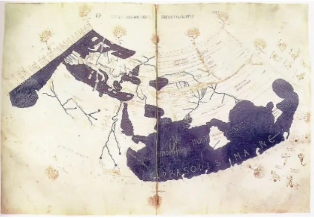
Visualization as a discipline to present information is not a recent phenomenon. Before the so-calledinformation society, visualisation techniques were used in maps and scientific drawings for over a thousand years.

Figure 1.1: ThePtolemy world mapas an example of data representation.

In this chapter we provide a generic overview about computer visualisation, in partic-ular in relation to medical visualization. Then, we set out the boundaries for the problem we are studying and finally we point out the organisation of the remaining chapters in this dissertation.

1.1 Visualization Overview

(18)

1. INTRODUCTION 1.1. Visualization Overview

investigate a huge amount of data, we can use computer generated graphs or images. Visualization itself has already proved to be a powerful tool for data investigation in the past so the know-how accumulated for many centuries has been transferred to computer visualization.

The emphasis on computer visualization started in the early 1990s with the special issue of Computer Graphics on Visualization in Scientific Computing. Since then, multiple conferences solely focusing on visualization have been organised. Two of then are the

Eurographics Workshop on Visualizationand theIEEE Conference on Visualization.

Despite initial differences that were set up according to the information to be repre-sented, that is, whether it was scientific numerical data or more generic non-numerical data, we are witnessing a more common approach to data visualization. Hence, the fields ofScientific VisualizationandInformation Visualizationare getting more and more interre-lated.

In order to illustrate the importance of visualization nowadays, we list below some important applications:

Medical visualization. Anatomic data is acquired through scanning device machines, which is then presented using a volume visualization technique, for instance isosurface extraction. This kind of applications can be used to help physicians to diagnose cancer for example.

Flow visualization. The objective is to make flow patterns visible. Most fluids (air, wa-ter, etc.) are transparent, thus their flow patterns are invisible to us without some special methods to make them visible. The data can be obtained by flow simulation or by mea-suring experiments. The design of new aircrafts can be validated by using simulations with flow visualization. In this way, there is no longer a need to construct expensive pro-totypes in order to test the project design.

Geographic information systems. For a long time maps have been used to visualize geographic data. Techniques like height fields or isolines are commonly used in com-puter visualization to show topographic information like mountains.

Information visualization. One of the focus is to use computer-based tools to explore large amount of data. Big databases and multi-modal data increasingly require appropri-ate visualization techniques. For example, business data visualization is widely used to represent economic data.

(19)

1. INTRODUCTION 1.1. Visualization Overview

Large-scale data visualization. It is particularly used when studying natural phenom-ena. For example, earth sciences turbulence calculations can produce large amount of data, leading to huge demands on power computation. Astrophysics is another example which deals with data measured at a huge scale so no direct data investigation is possible. Some techniques used in large-scale data visualization have to deal with data reduction, sometimes trading data resolution for some level of user interactivity.

The first application we have mentioned above – Medical visualisation – is an important part of the visualisation field. It is also the one where our work fits in. In the following we will extend this subject.

After the x-ray technology was invented in the 19th century, it was then clear that it would be a valuable diagnostic tool. Nevertheless, the x-ray technology was still limited as physicians had to work with a minimal set of images.

Once computed tomography (CT) and Magnetic Resonance (MR) were introduced, we were able to work with larger set of images from a given patient and to have a more detailed view of his body. The amount of images was still limited, but the traditional light boards started to become small to contain all the images, thus making it harder to analyze the patient body. With the rise of computational power, computers helped to solve the problem. By the end of the 1990s, computers were just an alternative to the light board.

When the first multi-slice CT scanners were introduced, there was a new task for computers: to create a 3D representation of the anatomical structure pictured in the im-ages provided by these scanners. It was a perfect solution, as the huge amount of imim-ages obtained were too hard to analyze one by one, and consequentely it was hard to get an overall description of the patient’s body. Fortunately a 3D representation would help to solve these problems.

With the rise of medical visualization, also new ways to visualize volumes in medicine have emerged. For example:

Diagnostics. With 3D medical visualization, new ways to diagnose patients have been found. This is the case of Virtual Endoscopy, which avoids the painful process the patient would have to face by using a real endoscope. An example of a virtual endoscopy is shown in Figure1.2.

Communication. 3D medical visualization now helps the communication between the radiologists, surgeons and patients. It is a fact that 3D renderings are much easier to understand by people.

(20)

1. INTRODUCTION 1.2. Problem Description

Training. Students and doctors can be trained with the help of a virtual training envi-ronment.

Figure 1.2: Virtual Endoscopy of the colon (virtual colonscopy) [MITa].

1.2 Problem Description

Some anesthesias (e.g. epidural anesthesia) can be hard to administer by doctors, partic-ularly when they are professional juniors. Teaching a doctor or student the behavior of the anesthesia along with the location in which it must be administered can be an hard process.

Most of the available 3D medical applications don’t allow the representation of time-varying data volumes. Because of this, there isn’t much support when it comes to anes-thesiology acts. Furthermore, most of the research in the area of medical visualization is focused in the fields of diagnostics and surgical planning.

The main purpose of this dissertation is to provide a tool that allows students or young doctors to study anesthesiology acts. This tool should create a 3D representation of an anatomical structure along with the anesthesia substance. Also, it should incorporate an appropriate annotation system to facilitate the studying process.

(21)

Figure 1.3: Surgical plan of a neurosurgery [vdB].

time.

In order to answer positively to the requirements we have set out, we first must iden-tify our main challenges and to establish how we can overcome them.

Before physicians started using 3D imaging software, they used to analyze the pa-tients with the 2D images from CT or RM scanners. As the computational power has increased, 3D imaging started being used more often and it became an active area of re-search in computer science. Today we have multiple ways of representing the human body in 3D from data acquired using medical imaging machines. Although a lot of re-search has been done, to the best of our knowledge there is no software allowing doctors or medical students to study the behaviour of anesthesia substances in the human body.

As it was mentioned, there are multiple methods to represent the human body in 3D. These methods have their own advantages and disadvantages, and so one of the problems we are facing revolves around choosing the best methods to create our tool. We envisage four major areas to look at:

• User interface and basic visualization.

• Image segmentation.

• Rendering of data volume.

(22)

User interface and basic visualization.This part of the problem consists of designing a proper user interface with the potential of satisfying all user requirements. For exam-ple, we have to decide what menus and what types of visualization will be available.

Image segmentation. As previously stated, 3D medical imaging software usually goes through a phase of segmentation, so our application will not be different. There are sev-eral segmentation methods available, some of them are more suited to our problem than others. For instance, for our problem we are interested in those that work better with soft tissues. There are other aspects we must also take into account when choosing the segmentation method. For example, how accurate is the method, how sensitive is the method to noise, etc. The level of interactivity in the segmentation phase is also a major concern. The physician must be able to validate the segmentation and, in case the seg-mentation is faulty, he must be able to make proper adjustments in the used segseg-mentation method used.

It is crucial that this phase of the problem is well addressed because the next phases depend a lot on this one.

Rendering of data volume. This phase depends on the image segmentation phase. At this point, the components identified in the segmentation phase are used to create the corresponding 3D model. To do this, there are multiple approaches (e.g. volume ren-dering and surface-based renren-dering). We have to decide which approach better fits our objectives. The chosen approach must be of low computational complexity, because the physician must be able to examine a given anatomical structure from different perspec-tives and if using a complex rendering method might slow down this process. Although at first this might not seem very important nowadays because of the growth in CPU/GPU power, we must also take into account that, in the next phase, we need to represent a time-varying data volume. The representation of multiple members identified in the segmen-tation phase must be well distinguishable. It is a fact that it is necessary to differentiate the anesthesia from the anatomical structure at hand.

Rendering of time-varying data volume. Because we want to be able to analyze the be-haviour of the anesthesia, it is necessary that such bebe-haviour varies as time passes. That is what happens in reality. The main issue here might be the size of the data set used, even though we do not expect to have very large data sets during the testing phase. However, that doesn’t mean it will not be the case in the future.

(23)

1. INTRODUCTION 1.3. Dissertation Organization

1.3 Dissertation Organization

The remaining chapters in this dissertation are organized in the following way:

We start Chapter2by analysing work that might be related to ours. The main themes are segmentation, rendering and time-dependent visualization. In the segmentation sec-tion we present basic segmentasec-tion algorithms and algorithms widely used in medical visualization. In the rendering section we present the marching cubes algorithm and vol-ume rendering techniques. Regarding time-dependent visualization, we present some of the main problems and suggested techniques to solve these.

In Chapter3– Lumbar region segmentation – we discuss the techniques used during the segmentation of the lumbar region and the reasoning behind it. The whole segmenta-tion process goes through 3 main stages:pre-processing, which addresses noise reduction,

algorithm initialization, which demonstrates some of the necessary intermediate steps we have to go through to run a segmentation algorithm successfully and finally the segmenta-tion, which deals with choosing and applying segmentation algorithms. The anatomical structures segmented are the abdominal aorta, back muscles, spinal canal and the verte-bral body.

Chapter 4 – Time-Dependent rendering – presents and compares two approaches used to segment and render time-dependent datasets. The first approach tries to pro-cess each of the time slices one at a time while the other has no defined order to propro-cess the time slices (parts of each time slice can be processed instead of a whole slice) and simply presents the final results at the end.

Chapter 5 – Prototype – presents the architecture used to build the prototype and demonstrates how the interface works given that the user wants to segment a certain anatomical structure and interact with, or modify the segmentation.

(24)

(25)

2

Related Work

In this chapter we present some related work covering aspects of data segmentation, rendering, time-varying visualization and development toolkits.

First, we start by introducing the framework of the data visualization process. Then we lay out some aspects of data acquisition, followed by a discussion about some tech-niques for image pre-processing. Then we present segmentation algorithms, whether being the general ones or the ones commonly used in medical imaging. Next, we discuss 3D visualization techniques, both in terms of volume and surface-based visualization. We then make reference to the difficult issue of time-varying visualization. Finally, we present a set of toolkits that can be used to develop a tool for medical visualization.

2.1 Data Visualization Process

The data visualization process can be described according to the pipeline presented in Figure2.1.

Figure 2.1: The Data Visualization pipeline[cp].

(26)

2. RELATEDWORK 2.2. Data Acquisition

the method can be a CT or MR scanning. In other kinds of applications (e.g. flow visual-ization), the raw data can be obtained through a simulation.

To make theRaw Datauseful,Data Transformationsneed to be applied in order to cre-ate a set ofProcessed Data. Examples ofData Transformationsare statistical computations like averaging values. Operations like data stratification or orderingRaw Databy some attribute can also be made at this stage of the visualization process. If there are problems like errors in data, they must be detected and addressed right at this stage in order to avoid presenting erroneous information to users.

Then, a mapping function is applied to theProcessed Data in order to create aVisual Structure. At this stage, it is important to consider the goal of the visualization so a proper mapping function will be used. For example, statistical representation (e.g. histograms) is a classic technique to buildVisual Mappings.

Finally,View Transformationscan then be applied interactively in order to modify rep-resentations. An example of a transformation made at this stage isZooming.

2.2 Data Acquisition

Medical data acquisition, as the first stage in the visualization pipeline (see Figure2.1), is particularly concerned with the technologies used to acquire data sets of the anatomical structure of a given patient. In the following, we present some of the most important technologies considering our problem.

2.2.1 Computed Tomography

Computed Tomography (CT) was the first imaging technique to generate slice images and therefore it became a very important technology in 3D visualization.

Figure 2.2: A CT Scanner [Hos].

(27)

2. RELATEDWORK 2.2. Data Acquisition

through the patient’s body. The value obtained by the last detector is then compared to the radiation tracked by the reference detector in order to check how much did the radiation weakened.

2.2.2 Magnetic Resonance Imaging

Magnetic Resonance Imaging (MRI) is also an important imaging technique in 3D visu-alization. Similarly to CT, this method can also generate slice images. An MRI scanner contains a powerful magnet which is used to align the magnetization of some atomic nuclei in the body. Radio frequency fields are then used to alter the alignment of this magnetization. This causes the nuclei to produce a rotating magnetic field detectable by the scanner. This information is used to construct and image of the scanned area of the body.

2.2.3 Positron Emission Tomography

Positron Emission Tomography (PET) is an imaging technique that produces a 3D data volume of functional processes in the body (a radioactive tracer is used to show chemi-cal activity of anatomichemi-cal structures). To produce a 3D data volume, the system detects gamma rays emitted indirectly by a positron-emitting radionuclide, which is introduced into the body. The 3D volumes are then constructed by using computerized reconstruc-tion procedures, like the ones used in CT and MRI.

2.2.4 Discussion

As expected, the data acquisition technologies we have mentioned above have their own advantages and disadvantages.

Computed Tomography is suited to detect bone injuries, chest imaging and cancer detection. This technique is widely used in emergency room patients. When it comes to details of bony structures, CT provides a good detail. Although with less detail, it is also able to depict soft tissues and blood vessels.

Magnetic Resonance Imaging is suited for soft tissue evaluation such as ligament and tendon injury, spinal cord injury and brain tumours. However, it is worth to point out that bony structures are not as detailed as soft tissues.

(28)

2. RELATEDWORK 2.3. Image Pre-processing

2.3 Image Pre-processing

Before applying a data segmentation algorithm, sometimes it is necessary to denoise the image as the segmentation algorithm to be used may be too sensitive to noise. If there is no proper care then the resulting segmentation will have poor quality. In this section we present two smoothing methods widely used: edge preserving smoothing and median filter.

2.3.1 Edge Preserving Smoothing

The main problem of smoothing/denoising is that it tends to blur away sharp bound-aries in the image that could help to distinguish anatomical structures. Perona and Malik [PM90] introduced a method called anisotropic diffusion. With this technique it is possi-ble to reduce image noise while preserving or even enhancing edges in the image. This was possible by introducing a variable diffusion coefficient (which was constant before). This way it is possible to limit the amount of smoothing near edges or boundaries. The

anisotropic diffusionequation if given in equation2.1, where I(x, y, t)is the image inten-sity, div and∆are the divergence and gradient operators, andc(x, y, t) is the diffusion coefficient.

∂

∂tI(x, y, t) =div(c(x, y, t)∇I(x, y, t)) (2.1)

The diffusion coefficient must encourage the forward diffusion inside smooth regions and backward diffusion at high gradient locations. Perona and Malik [PM90] proposed multiple mathematical functions for the diffusion coefficient, being equation2.2 one of them. The parameterk, theconductance parameter, controls the sensitivity of the process to edge contrast.

c(x, y, t) = exp −

|∇I(x, y, t)|2

k

!

(2.2)

This particular equation takes advantage of the high contrast edges rather than the low contrast ones.

2.3.2 Median Filter

The median filter can also be used as a robust approach for noise reduction. The filter is particularly efficient against salt-and-pepper noise2.3. The median filter computes the value of each output pixel as the statistical median of the neighborhood of values around the corresponding input pixel. A radius for each dimension must be provided to create a neighborhood.

(29)

2. RELATEDWORK 2.4. Generic Segmentation Algorithms

Figure 2.3: Example of salt-and-pepper noise [Blo].

Figure 2.4: Median filter example [HJJtISC13].

This method tends to not damaging the boundaries and edges too much and it is of very little complexity. It is also known that, by applying the algorithm multiple times with the same radius, we can obtain results fairly similar to the ones that we obtain using theanisotropic diffusionfilter mentioned above.

2.4 Generic Segmentation Algorithms

Image segmentation is the process of partitioning an image into multiple segments. This is a crucial task in medical visualization. The goal is to change the representation of the image in order to ease the identification of the objects of interest in the image and thus, to make the overall image analysis much easier. An image segmentation technique usually assigns labels to the image pixels and the pixels with same label share certain visual characteristics.

When applied to a stack of images, which is a typical scenario in medical imaging, the resulting contours after image segmentation can then be used to create 3D represen-tations.

In the following we present some of the basic segmentation algorithms. As a first objective, we have to understand how basic segmentation can be done.

2.4.1 Thresholding

(30)

Figure 2.5: Thresholding of an image with a bi-modal intensity distribution [oE].

Figure 2.6: Thresholding of an image with a multi-modal intensity distribution [oUSoc].

Inglobal thresholding, there are two groups of pixels: The group 1 corresponds to the set of pixels that have an intensity value greater or equal to the threshold valuet; the rest of pixels (the ones with an intensity value lesser thant) belong to group 2. The complexity of this algorithm is very low, but because of this, it brings us some shortcomings. Global thresholdingworks fine with images with a bi-modal distribution (see Figure2.5) but, as we can see in Figure 2.6, the algorithm will perform poorly if the image has a multi-modal distribution. To obtain better results with images with a multi-multi-modal distribution, entropy based threshold algorithms were suggested in [PSY97]. These algorithms try to maximize the entropy in the thresholded image. That is, in images with bigger contrast between pixels, we can obtain better segmentation results using threshold techniques. An alternative to entropy based algorithms are the histogram shape based threshold al-gorithms [CL98], which try to force multi-modal intense distributions into a bi-modal distribution.

Instead ofglobal thresholding, we can uselocal thresholding. This local method divides an image into sub-images and selects an independent threshold value for each sub-image. This technique is very sensitive to noise and some of the segmented regions might not correspond to the objects in the original image.

(31)

2.4.2 Region-based Segmentation

Region-based image segmentation rely on grouping similar neighbouring pixels. There are two main methods:split and merge[CP80] andregion growing[AB94].

2.4.2.1 Split and Merge

Thesplit and mergemethod divides an image into multiple regions and then merges the ones that are similar according to some criteria (see Figure2.7). To be more precise, the whole image is first considered as a single region. If a certain homogeneity criterion is not met, then the region is split into four quadrants. This process is repeated recursively within each region. When each of the regions contain only homogeneous pixels, the al-gorithm starts comparing all regions with their neighbor regions and merge the ones that are similar. It is an algorithm computationally fast.

Figure 2.7: Split process of the Split and Merge algorithm [oUDoB].

2.4.2.2 Region Growing

The region growing method works in the opposite way relative to the split and merge

method. It begins by selectingnseed pixels. The algorithm will then try to merge each of these pixels with similar neighbors (pixels with similar intensities) so creating a region of multiple pixels. An illustration of this process is shown in Figures2.8and2.9.

R. M. Haralick and L. G. Shapiro have proposed a variant of this technique [SH01]. Basically the mean and variance of a region are used now to decide if a pixel belongs or not to that region.

(32)

Figure 2.8: Region Growing algorithm: Start of a growing region [oCSI].

Figure 2.9: Region Growing algorithm: Growing process after a few iterations [oCSI].

2.4.3 Edge-based Segmentation

Edge-based segmentation algorithms use edge detectors to create segments in a given image. This helps to distinguish the multiple structures in an image. Examples of such algorithms, presented below, are the gradient magnitude filter and the canny edge detec-tor.

2.4.3.1 Gradient Magnitude

The magnitude of the image gradient is extensively used in image analysis, mainly to help the determination of object contours and the separation of homogeneous regions. A gradient magnitude operator detects the amplitude edges at which pixels change their gray-level suddenly. For an image volume, the magnitude of the gradient vector assumes a local maximum at an amplitude edge. The magnitude is zero if the volume is constant. Equation2.3can be used to calculate the magnitude for a volumef(x).

|∇f|=

s

(∂f

∂x)

2_{+ (}∂f

∂y)

2_{+ (}∂f

∂z)

2 _(2.3)

(33)

point in the image, the result is either the corresponding gradient vector or the norm of this vector.

In the case of 2D, the operator uses two 3x3 matrices (masks), which are applied to the original image to calculate the approximations of the derivatives. One of the matrices is used for horizontal changes and the other one for vertical. LetAbe the source image,

GxandGythe images that contain the horizontal and vertical derivative approximations:

Gx= 

 

−1 0 +1





 andGy = 

 

+1 +1 +1 0 0 0

−1 −1 +1





 (2.4)

Both images, (GxandGy), can be combined using equation2.5.

G=qG2

x+G2y (2.5)

2.4.3.2 Canny Edge detector

An example of detector is theCanny Edgedetector [Can86], which uses a double thresh-olding technique. After going through a smoothing step, the algorithm finds the edge strength by taking the gradient of the image. The Prewitt operator (see Equation2.4) can be used to approximate the absolute gradient magnitude (edge strength). The edge di-rection must also be calculated. To do this we can simply use Equation2.6, whereθis the angle (which corresponds to the edge direction) andArctan()is the arctangent. Finally, a thresholdt1is used to detect edges by comparing the pixels in the image with the

thresh-old. Any pixel that has a greater value thant1is presumed to be an edge pixel. Another

thresholdt2is defined as a criterion to connect possible edges to the already defined edge

pixel. Any pixels that are connected to the edge pixels defined byt1 and have a greater

value thant2 are also selected as edge pixels. Figure2.10shows a result of this detector.

θ=Arctan(Gy/Gx) (2.6)

Edge-based segmentation algorithms tend to find edges which are irrelevant to the object, and the contours of the object sometimes are disjointed. Edge-based segmenta-tion algorithms usually have low computasegmenta-tional complexity.

2.4.4 Graph-based Segmentation

Graph-based segmentation consists in the formation of a weighted graph, where each vertex corresponds to a region in the image. The edges are weighted with respect to some measure. Graph-based algorithms often try to minimize cost functions such as acut

(34)

2. RELATEDWORK 2.5. Common Segmentation Algorithms for Medical Imaging

Figure 2.10: Example of result of the Canny Edge detector [vddcAUp].

i.e., the edge in the graph between two similar pixels (which will be represented by two vertexes) will have a high weight value and the connection between two very distinct pixels will have low weight, i.e.,G= (V,E) whereVis the set of vertexes and E the set of edges andAandBtwo disjoint sets ofV, we have the cut function:

cut(A, B) = X

a∈A, b∈B

w(a, b) (2.7)

Because similar pixels are connected with high weight edges and the distinct ones are connected by low weight edges, by minimizing thecutfunction, the partitionsAandB

are created and will represent two segments in the image.

Graph-based segmentation algorithms usually find global optimal solutions. As ex-pected, these algorithms are computationally expensive.

The segmentation methods we have presented in this section are all very similar when it comes to complexity, with the exception of graph-based segmentation, a complex one. While region-based and graph-based methods can cause over segmentation, edge-based can create disjoint edges and thresholding depends on the intensity distribution.

Despite all that, these algorithms can be tailored and combined together to achieve better results in medical image segmentation. But if generic implementations are used, then the boundaries obtained will not necessarily correspond to the real boundaries we aim to find out.

2.5 Common Segmentation Algorithms for Medical Imaging

Medical images might pose specific needs and challenges when comparing to other type of images. Above all, we need to understand which type of algorithms are more helpful for our work and which ones are less helpful.

(35)

theatlas-based segmentation. We expect that other methods with similar characteristics will deliver similar efficiency and quality.

2.5.1 Active Contour Model

Active contour model, or snakes, proposed by Kasset al.[WT88], consists of a deformable geometric spline which is influenced by image forces and other constraint forces. These forces pull the spline towards object contours. A snake can be defined parametrically as

v=v(s) = (x(s), y(s)), s∈[0,1]. (2.8)

The matching between the snake and the image is made by means of energy mini-mization. The total energy of the snake can be written as

E∗ snake=

1 Z

0

Esnake(v(s))ds=

1 Z

0

(Einternal(v(s)) +E_image(v(s)) +E_con(v(s)))ds (2.9)

where Einternal represents the internal energy, Eimage represents the image forces and Econrepresents the external constraint forces. The internal energy can be written as

Eint= (α(s)|v_s(s)|2+β(s)|v_ss(s)|2)/2. (2.10)

The first order term represents the stretching force of the snake and the second order term represents its bending force. Large values ofα(s)will increase the internal energy of the snake the more it stretches, if the value ofα(s)is small, the energy function will be insen-sitive to the amount of stretch. Simillarly, large values ofβ(s)will increase the internal energy of the snake the curves it has, if the value ofβ(s)is small, the energy function will be insensitive to curves in the snake.

The image energy can be written as

Eimage=wlineEline+wedgeEedge+wtermEterm (2.11)

Adjusting the weights will determine which features will be considered by the snake.

Eline is the intensity of the image, which can represented byEline = I(x, y). Adjusting

the sign ofwlinewill make the line attracted to dark lines of light lines. Edges in the

im-age can be found by following an energy function which makes the snake attract towards contours with large image gradients. Eedgecan be represented byEedge = −|∇I(x, y)|2.

The constraint energyEcon can be used to interactively guide the snake.

(36)

broken edges and subjective contours. While the original snake model cannot converge well to concave features, GVF also solves this problem.

The values ofαandβof the internal energy are chosen subjectively. Gaoet al.[JGK98] proposed a solution to define these values in the extraction of the liver boundary. After a preprocessing phase, which include steps like removing the noise of the original images, the liver boundary is refined by snake algorithm. The value of αis proportional to the distance of adjacent control points, andβis inversely proportional to the curvature value.

2.5.2 Level set methods

Level setswere firstly introduced by Osher and Sethian [OS88] and have been widely used in medical image segmentation. This is mainly due to their ability to track the boundaries of the biological structures of interest. It is worth to point out thatactive contourscan be implemented usinglevel sets.

Thelevel setsmethod creates a contourΓ(t), which evolves towards the boundaries of the desired object. It is defined as the zero levo set of and embedding functionφ(x, y, t) :

R3_→_R_{as given in equation}_2.12_.

Γ(t) ={(x, y)|φ(x, y, t) = 0} (2.12)

Using the contour defined in equation2.12, we can define two domains:Ω+₌_{₍_{x, y}₎_|_φ₍_{x, y, t}₎_>

0}, which is the interior of the contour, andΩ−₌_{₍_{x, y}₎_|_φ₍_{x, y, t}₎_<₀_}_{, the exterior.}

The level set functionφ(x, y, t)can be defined using the euclidean distance function. Equation2.13shows a possible definition. The distanced(x, y, t)is defined as the length of the shortest path from point(x, y)to the desired contour.

φ(x, y, t) =

  

 

−d(x, y) :(x, y)∈Ω−

0 :(x, y)∈Γ(t)

d(x, y) :(x, y)∈Ω+

(2.13)

With the level set function defined, we can now introduce the outer unit normal vector

− →

N (equation2.14)

− →

N =− δφ

|δφ| (2.14)

The contour will evolve in time due to several artificial forces, which makes the con-tour move in the normal direction.

2.5.2.1 Fast Marching

(37)

describes the evolution of a closed curve as a function of timeT with speedF(x)in the normal direction at a pointxon the curve. Concerning the time function in the equation, the user can specify at which time the algorithm stops (this is used to save computational time). The user must also provide at least one seed point with an initial value.

F(x)|∇T(x)|= 1 (2.15)

The speed function values are usually obtained from a speed image. The main pur-pose of this image is to use it as an indicator of where the level sets function should grow faster and where it should grow slower. Suppose we have an image which intensities are between the values 0.0 and 1.0. Ideally the speed value should be 1.0 in homogeneous regions of anatomical structures and the values should decay rapidly to 0.0 around the edges of structures. There are several methods to produce a speed image. For instance, we can use the sigmoid filter. The sigmoid filter gives us more control over the resulting speed image because of its parametersαandβ.

The sigmoid filter is based on the sigmoid intensity transformation (see equation2.16). This filter is commonly used as an intensity transform: It maps a specific range of inten-sity values into a new inteninten-sity. Because the sigmoid is a non linear function, it is possible to focus attention on a particular set of values, while progressively attenuating the values outside that range. The parameterαin equation2.16defines the width of the input in-tensity range andβdefines the intensity around which the range is centered (see Figure

2.11).

I′

= (M ax−M in)∗ 1

1 + exp(−(I−β_α ))+M in (2.16)

Figure 2.11: Influence of the alpha and beta parameters in the sigmoid func-tion [HJJtISC13].

(38)

2.5.3 Active Shape Model

Organs and other biological structures in medical images have a tendency towards some average shape. This tendency can be very useful when proposing algorithms.

Cootesel al.[TFCJ94] proposed to useActive Shape Modelsin order to locate structures in medical images. This method requires a training phase in order to take advantage of the average shape of a biological structure.

Once the training phase is finished, the algorithm appliesPrincipal Component Analysis

(PCA) to identify the relevant shapes. After this step, it is possible to create an arbitrary shape by the linear combination of these identified shapes. The outcome can then be deformed by changing the coefficients used in the linear combination. A similar method was used by Gleasonet al.[SSGM02] to detect poly cystic kidney disease in CT images. The main disadvantage of this algorithm is to require of a lot of training samples.

2.5.4 Atlas-based Segmentation

In some applications, a clinical expert can manually label several images and so seg-menting unseen images is a matter of extrapolating from these manually labeled training images. Methods like this are referred to as atlas-based segmentation methods.

The atlas construction can be based on a single object. The training images are used separately to construct the atlas, but this poses several problems. Since the selection of a sample is arbitrary, it means that the selected object may not be a typical one. Fur-thermore, the fact that only one sample is used, means that no information about the variability of the object is available so it is impossible to determine if the resulting shape is acceptable. To solve these problems,probabilistic atlashas been proposed [PBM03]. This method uses a spatial distribution of probabilities to determine if a pixel belongs or not to an organ. To obtain the probability distribution, multiple samples are used. Usually it is required the use of image registration in order to align the atlas images (the sam-ples) to a new image. Similarly to the active shape model (which can be considered as a probabilistic atlas), the disadvantage of probabilistic atlas is that it requires a large set of training samples in order to work properly.

(39)

2. RELATEDWORK 2.6. Volume Rendering

and active contour models also provide a greater level of interactivity since they don’t re-quire as much time to execute as atlas-based segmentation or other methods that rere-quire training.

2.6 Volume Rendering

Volume rendering is a rendering technique aiming to display a 3D sampled data set en-tirely, therefore laying emphasis on the overall as opposed to the detail. Usually, the data set is a group of 2D slice images acquired by a CT or MRI scanner. These slices are taken following a regular pattern (e.g. one slice every milimeter) thus allowing us to reconstruct the complete volume.

In the following we present the most important techniques used in volume rendering.

2.6.1 Ray Casting

Ray Castingwas introduced in 1988 by Marc Levoy [Lev88] and, as we can see in Fig-ure2.12, it generates high-quality images. In medical imaging, we can use ray casting in the field of virtual endoscopy [HO00] for example.

In this technique, a ray is generated for each desired image pixel. Originating from the camera position, multiple rays are traced through the data volume. Along the part of the ray that lies within the volume, equidistant samples are selected. If the volume is not aligned with the ray, sampling points will be located between voxels and it will be necessary to interpolate the values of the samples from its surrounding voxels. After all sampling points have been shaded, then the final color for the pixel currently being processed is computed. To do so, the sampling points are combined along the ray. In general, this composition starts with the samples farthest from the viewer and ends with the one nearest to him, in a blending fashion of layers. Masked parts of the volume do not affect the resulting pixel.

Ray casting used to be demanding technique, in particularly priori to recent advances in graphic cards technology. Several techniques have been proposed in the past to speed up the technique [RAW94,RGY98].

It is worth to point out that ray casting nowadays should be parallelized, that is, instead of casting rays in a sequential fashion, multiple rays should be casted at the same time, in parallel. Thanks to this, ray casting is now considered as an interactive technique.

2.6.2 Shear Warp

(40)

2. RELATEDWORK 2.6. Volume Rendering

Figure 2.12: Volume ray casting applied to CT data of a crocodile. The image was ren-dered by Fovia’s High Definition Volume Rendering engine [Wikb].

computer’s memory. Because the pixels have to be rearranged, the image is distorted and a final correction step is necessary (warping the image).

This technique is relatively fast in software at the cost of less accurate sampling and worse image quality when compared to ray casting. Nevertheless, the reasonable trade-off between speed and quality made it an interesting choice for implementation in special hardware architectures.

2.6.3 Splatting

Thesplattingtechnique was proposed by Lee Westover in 1991 [WW91]. This technique is meant to trade quality for speed. With splatting, volume rendering displays are com-posed by accumulating splatted data voxels on the viewing surface in back to front order. The degree of influence of each voxel is defined by a reconstruction filter.

The all process resembles the result of throwing snow balls on a wall.

2.6.4 Maximum Intensity Projection

Unlike the accumulation process of other volume rendering techniques, the maximum in-tensity projection method only picks out and projects the voxels with maximum inin-tensity that fall in the way of parallel rays traced, from the viewpoint to the plane projection.

This technique is a widely used technique in medical visualization. For example, it is the rendering technique of choice when it comes to the investigation of vascular structures [CWQ+

(41)

2. RELATEDWORK 2.7. Surface Rendering

2.7 Surface Rendering

While volume rendering is concerned with the display of the data sets in their entirety, surface-based rendering techniques focus on depicting surfaces within the volume. Hence, it is a useful technique to emphasize material transitions within the volume, as depicted in Figure2.13.

In the following we present the common surface-based rendering techniques. In par-ticular, iso-surface extraction and segmentation masks.

As a historical note, we should make reference to the technique called contour ap-proaches. They were widely before the introduction of iso-surfacing techniques but not anymore. Basically, in a semi-automatic or manual way, the 2D contours (points of same value but in a 2D slice) of the structures of interest were identified on single slices. Then geometric algorithms were used to connect the contours of adjacent slices in order to form a closed surface [KSSe00].

Figure 2.13: An example of a surface-rendered human skull [Ren].

2.7.1 Iso-surface extraction

Iso-surface extractionaims to represent all points within a volume with the same property or value. The Marching Cubes (MC) technique is the best established iso-surface extrac-tion approach. It was introduced by W.E. Lorensen and H.E. Cline in 1987 [LC87] and since then it has been broadly used in various domains.

With the rectangular volume data defined as a set of voxels, the algorithm starts by examining each of these voxels, one by one. Each voxel has eight neighbor locations, thus forming an imaginary cube. Then the algorithm determines the polygon or polygons needed to represent part of the isosurface that passes through the cube. The polygons are then used to produce the desired surface.

(42)

2. RELATEDWORK 2.8. Time-Varying Visualization

along the cube’s edge by linearly interpolating the two scalar values that are connected by that edge. This time consuming process motivated researchers to come up with sev-eral acceleration strategies [IK94,LA98]. Moreover, there were some issues related to the accuracy of the initial solution, which led to further research work [LB03].

Figure 2.14: The original 15 MC configurations, considering both rotational and reflective symmetry. These configurations led to further research to address issues of accuracy so they have been extended [Wika].

2.7.2 Segmentation Masks

This technique simply consists of displaying regions of the data volume which have been identified by segmentation techniques. Therefore it is just a matter of representing graph-ically the points already identified. Unlike iso-surface extraction, there is no need to process the all volume data. But in this surface-rendering method, special smoothing techniques have to be employed because segmentation masks usually originate staircase artifacts.

2.8 Time-Varying Visualization

Most of the applications in 3D visualization use a single data set that corresponds to a single instant of time of its domain of interest. Such data set is of dimension width× height×depth.

However, when referring to time-varying visualization, as it happens in medical vi-sualisation, we have to deal with an extra dimension: The time. As a consequence, the data set dimension is nowwidth×height×depth×time.

(43)

2. RELATEDWORK 2.8. Time-Varying Visualization

Philip Sutton and Charles D. Hansen proposed the use of Temporal Branch-on-Need Trees (T-BON [SH99b]. In the preprocessing step, a branch-on-need octree for each time step in the data, the tree infrastructure is stored to disk. Before any isovalue queries, the tree infrastructure is read from disk and recreated in main memory. After this, queries are accepted in the form(timestep, isoval). The values of the nodes corresponding totimestep

are first read. If the values spanisoval(i.e. greater than theisoval), the children of these nodes are read. If a lead node spansisoval, the disk block containing the data for the cells in that leaf is added to a list. Once the necessary portions of the tree have been brought into memory, all blocks in the list are read from disk. This was proposed in 1999, when the memory capacity and computer power was much lower then it is today, which means that this algorithm can be tailored to read less data from the disk.

Han-Wai Shenet al.proposed a volume rendering technique which uses a time-space partitioning (TSP) tree [SH99a]. A TSP tree is similar to a regular octree. The difference is that the TSP tree node contains both spatial and temporal information about the under-lying data in the subvolume, while a regular octree only contains the spatial information. Zhe Fanget al.[FMHC07] suggested that the goal of medical diagnosis is not to ob-serve dynamic in real time as much as to differentiate healthy from diseased tissue. Hence it is not so important to provide interactive selection of arbitrary time-slices, but rather the comprehensive evaluation of the time-behaviour of each tissue sample and its classi-fication into different tissue types and tissue behaviours.

Zhe Fanget al.[FMHC07] also proposed a way of rendering time-varying medical im-ages by analyzing the time activity curve (TAC) of the voxels within a given volume. The TAC of each voxel is compared to a template TAC, which can be obtained by interactively probing the underlying data by specifying an arbitrary voxel via its spatial location, or it can also be generated from the result of some previous analysis, such as finding the average of a region of interest. The comparison between the template TAC and the other TACs results in a scalar value (i.e. each voxel associated with one scalar distance). The volume can then be rendered using classical (scalar) volume rendering algorithms.

Maet al. have provided a survey of different time-varying data visualization tech-niques used in large-scale data visualization [ML05].

(44)

2. RELATEDWORK 2.9. Development Toolkits for Medical Visualization

Finally, it is worth mentioning that most of the research in type-varying visualization is more common in areas other than medicine. For instance, in chemistry, mechanical engineering and other areas with various types of simulations. In medical visualization, the data sets tend to be smaller when it comes to time, because patients usually can not be exposed to PET or CT scanners for a long period of time.

2.9 Development Toolkits for Medical Visualization

In the following we present some of the most popular toolkits used to develop medi-cal visualization applications. This section ends with a brief discussion and comparison between such toolkits.

2.9.1 ITK – Insight Segmentation and Registration Toolkit

The Insight Segmentation and Registration Toolkit [ITK] is an open-source toolkit, de-veloped in C++ by several institutions and funded by the National Library of Medicine. It was developed mainly for image processing, segmentation and registration. ITK pro-vides a large number of segmentation algorithms such as thresholding, edge detection, region growing, active contour and watershed. Image visualization, manipulation or analysis features are not provided by ITK and so other libraries have to be used to cover these aspects. Also, ITK does not support 3D image rendering. But because of this, ITK provides interfaces to the Visualization Toolkit (VTK) [VTK], which can handle 3D image rendering.

2.9.2 MITK – Medical Imaging Interaction Toolkit

The Medical Imaging Interaction Toolkit (MITK) [MITb], developed at he German Cancer Research Center, combines ITK and VTK, thus easing the effort required to create applica-tions for medical image analysis. Notice that, as it was previously stated in Section2.9.1, ITK requires additional visualization and interaction features. The MITK community provides good documentation, as well as multiple tutorials and installation instructions to combine with Qt[Qt], a convenient tool to build graphical interfaces with MITK. Since MITK is derived from ITK and VTK, most of the ITK’s and VTK’s documentation can be used as well.

2.9.3 IGSTK – Image-Guided Surgery Toolkit

(45)

Figure 2.15: User interface of an application developed using IGSTK for robot-assisted needle placement in biopsies [AEC07].

2.9.4 User interface Development

As we can conclude from the sections above, it is necessary to use an additional library to build the user interface. The libraries wxWidgets [wxW], Fast Light Toolkit (TLTK) [FLT] and KWWidgets[KWW] are examples of open-source libraries which can be successfully used to build user interface for medical imaging applications. Even though not being open-source, Qt [Qt] provides a free version which can be used alongside ITK and VTK.

2.9.5 Application Builders

Multiple application builders and/or Problem Solving Environments (PSEs) have also been developed in the past. Such tools allow users to interactively design solutions to a certain class of problems, by providing a graphical interface where it is possible to build a processing pipeline. This is achieved by adding different modules and establishing a network of connections among them.

In this section we present some of the application builders that can support medical image analysis, processing and visualization.

DeVIDE.The Delft Visualization and Image processing Development Environments (DeVIDE) [DeV] provides several visualization and image processing features by inte-grating several libraries, such as VTK [VTK] and ITK [ITK]. It provides a higher-level function to ease their usage.

It is also possible to add new features to DeVIDE, by including new modules or adding code to existing ones in order to modify their behavior.

(46)

We notice that MeVisLab provides a helpful documentation tutorial.

SCIRun. SCIRun [SCI] is a problem solving environment developed at the Scien-tific Computing and Imaging Institute, University of Utah. Similarly to the application builders already mentioned, a user selects software modules and connected them in a visual programing environment in order to create a high level workflow. The modules include several ITK functionalities for image segmentation and registration, as well as it provides MATLAB integration.

It is worth mentioning that some of the applications developed at University of Utah have evolved from SciRun’s features, namely, Seg3D [Seg] and ImageVis3D [Ima].

ITK is a great tool for image processing and segmentation, even though it lacks visual-ization features. This can be fixed by also using VTK, MITK and IGSTK. We therefore can put together image processing methods, visualization and interface design, all in a single toolkit. With such framework, the developer’s effort is minimized. IGSTK seems to be a good choice when it comes to image-guided surgery.

(47)

3

Lumbar Segmentation

The lumbar region of the human body is one of the places where epidural anaesthesia is performed (see Figure3.1). There are several structures in this region that we believe are relevant during epidural anaesthesia, namely, the spinal canal, the vertebral body, the intervertebral disc, the abdominal aorta and the inferior vena cava.

Figure 3.1: Lumbar region of a human body.

(48)

3. LUMBARSEGMENTATION 3.1. Segmentation Pipeline

from image pre-processing to the segmentation itself. We evaluate results for the case of spinal canal, abdominal aorta, vertebral body and back muscles. This chapters ends with major conclusions we can draw from the tests carried out.

3.1 Segmentation Pipeline

The segmentation pipeline we set up for the purpose of image segmentation is depicted in Figure3.2. Hereafter we just consider MRI images.

Figure 3.2: Segmentation pipeline for a 3D MRI dataset.

After loading the MRI dataset to be analysed, the process starts with pre-processing of the images, having in mind the reduction of noise and the enhancement of the features of interest.

The next step is the related to initilization of algorithms. Actually, some segmentation algorithms require the use of additional filters to work properly.

The following step is the proper segmentation. At this point, we have used two types of algorithms, namely, the region growing and the level sets algorithm.

We should point out that there is usually an additional step at the end, where the obtained segmentation can be edited. However, as an interactive one, we have decided not to address it in this chapter.

Table3.1presents information about the datasets of the lumbar region that have been used in these experiments. They were taken from the lumbosacral region. The back muscles in these images are represented with low intensity values (notice that muscles can also be represented with high intensity values).

Name Size Inclination

MRIX LUMBAR 512 x 512 x 26 Axial R66y (901) 321 x 334 x 20 Axial R66y (801) 321 x 334 x 20 Axial MRIX LUMBAR 512 x 512 x 12 Sagittal LOMBIX 660 x 644 x 25 Sagittal LOMBIX 770 x 770 x 12 Sagittal A10y 435 x 432 x 11 Sagittal

Table 3.1: 3D MRI data sets of the lumbar region to be segmented. These images are all in the DICOM format.2

2

(49)

3. LUMBARSEGMENTATION 3.2. Image Pre-processing

As far as toolkits to help carrying out the experiments, and following the discussion presented in Section2.9, we have decided to use the Medical Imaging Interaction Toolkit (MITK) [MITb]. As mentioned, MITK is a free open-source software system for develop-ment of interactive medical image processing software. We will be also using the Insight Toolkit (ITK) [ITK] and the Visualization Toolkit (VTK) [VTK], since MITK combines both ITK and VTK as an application framework.

3.2 Image Pre-processing

As previously stated, the image pre-processing stage is used mainly to reduce noise and enhance image features. To denoise the image, we have used two main techniques: Me-dian filter andanisotropic diffusionfilter (as edge preserving smoothing). Both techniques are described in Section 2.3. The images presented in this section are from the dataset

MRIX LUMBAR[Osi] Axial.

3.2.1 Comparison

We have tested both methods with different parameters and values. Thesignal-to-noise

ratio was used to compare both methods, although it doesn’t take into account edge preserving characteristics. The equation3.1sets the computation of thesinal-to-noiseratio, whereµis the mean of the intensities in the image, andσthe standard deviation.

SN R= µ

σ (3.1)

Table3.2shows the results obtained for the median filter and for theanisotropic diffu-sionfilter. Thesignal-to-noiseratios obtained with the median filter are lower than those obtained withanisotropic diffusionfilter, as illustrated in Figure3.3. The median filter was used with the radius value of1to avoid damaging structure boundaries too much. The

anisotropic diffusionfilter was used with conductance parameter of1.0.

In this particular image, the fact thatanisotropic diffusionfilter doesn’t change the mean of the image, helps thesignal-to-ratioratio to grow faster than the one obtained with the median filter.

Note that if we kept increasing the number of iterations, thesignal-to-noiseratio ob-tained with the median filter would eventually surpass thesignal-to-noiseratio obtained with theanisotropic diffusion. This is because median filter is a linear smoothing filter and doesn’t take into account the boundaries of the structures in the figure, even though we can obtain good edge preserving results in some cases.

Figure 3.4show the images obtained for each of the filters using 35 iterations. The boundaries in the image obtained by the median filter were damaged and some have disappeared. Hence, we conclude that the median filter works better when there is less

(50)

3. LUMBARSEGMENTATION 3.3. Initialization

Median filter Anisotropic diffusionfilter

Iterations µ SN R µ SN R

5 162.978 1.144 168.318 1.155

10 161.636 1.149 168.318 1.188

15 160.791 1.153 168.318 1.209

20 160.153 1.156 168.318 1.225

25 159.628 1.158 168.318 1.238

30 159.189 1.160 168.318 1.250

35 158.820 1.162 168.318 1.260

Table 3.2: Mean and SNR results for both median andanisotropic diffusionfilters.

Figure 3.3: Median filtervs.anisotropic diffusionfilter.

noise in the image. If so, less iterations are needed to smooth the image, which means that there is a greater chance to preserve the boundaries of the structures.

Anisotropic diffusionusually takes longer to execute than the median filter. It may be an issue if there are time constraints at the segmentation stage.

On the basis on the results gathered, we are in favour of usinganisotropic diffusionin our experiments.

3.3 Initialization

Some segmentation algorithms, namely level sets, require additional initialization other than applying smoothing methods. The level sets method usually requires a speed image to be provided at the beginning. The intensity values in a speed image are interpreted as the values of a speed function used by the level sets (see Section2.5.2.1).

(51)

Figure 3.4: Original image (left). Use of median filter with 35 iterations and radius 1 (center), andanisotropic diffusionfilter with 35 iterations and 1.0 as conductance parameter (right).

can easily stop when the values start dropping to low intensity values.

3.3.1 Edge Detection Filters

The task ahead of obtaing the speed image itself is to apply edge detection filters. We have used two filters for that purpose: the gradient magnitude filter and thecanny edge detector.

3.3.1.1 Gradient Magnitude Filter

The gradient magnitude filter can be used as an edge detecting filter. Unless we use the gradient magnitude filter with smoothing, no additional parameters are required. Since we already went through a smoothing process, we have decided to use the gradient magnitude filter with no additional smoothing.

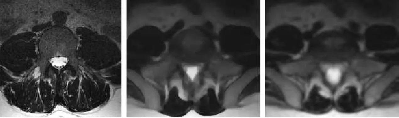
Figure3.5shows the resulting image after applying the gradient magnitude filter to the smoothed image of the lumbar region. But if no smoothing is applied, then the edges become mixed with the noise, as depicted in Figure3.6.

3.3.1.2 Canny Edge Detector Filter

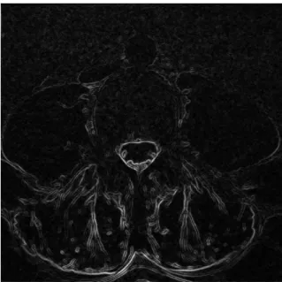
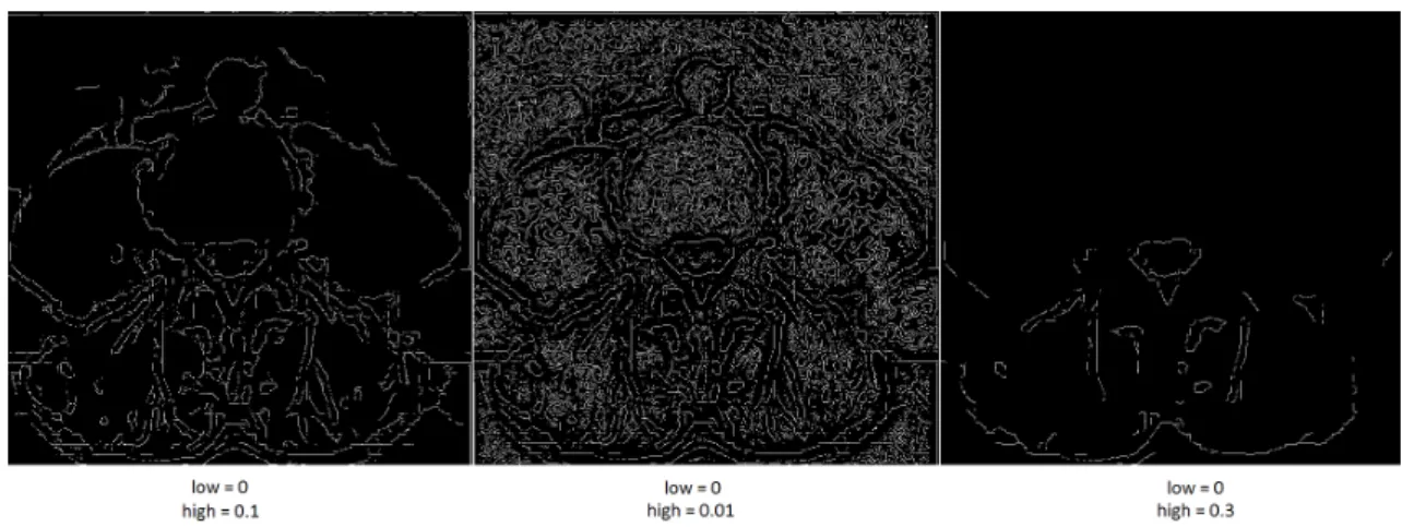
Another algorithm we have used to detect the edges was the canny edge detector. This method requires both a low threshold value and a high threshold value. The values must be less than 1 and negatives values will not work, which means thatlow < high <1.

(52)

Figure 3.5: Gradient magnitude filter applied after smoothing the image.

Figure 3.6: Gradient magnitude applied but without smoothing the image first.

3.3.1.3 Comparison

Regarding the execution time, it is a non-issue for both methods. Indeed, they both exe-cute very fast and so execution time is negligible.

The canny edge detector filter fails to completely connect some of the edges, while the gradient magnitude does this very well.

(53)

Figure 3.7: Canny edge detector results.

which simplifies the whole process.

3.3.2 Speed Image

As mentioned, a speed image is an image which values are interpreted as values of a speed function. Its main purpose is to be used as an indicator of where the level sets function should grow faster and where it should grow slower. Suppose we have an image which intensities are between the values 0.0 and 1.0. Ideally, the speed value should be 1.0 in homogeneous regions of anatomical structures and the values should decay rapidly to 0.0 around the edges of structures.

There are several methods to produce a speed image. For instance, we can use a sig-moid filter and, as an alternative, a reciprocal filter. We have used both for that purpose.

3.3.2.1 Sigmoid Filter

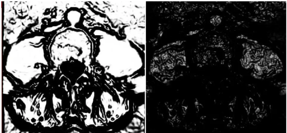
The sigmoid filter maps a specific range of intensity values into a new intensity. Because the sigmoid is a non linear function, it is possible to focus on a particular set of values, while progressively attenuating the values outside that range.

We can approach the problem of creating the speed image in two different ways: we can focus attention on the values of edges or alternatively on the values of homogeneous areas. The parameterβ is used for this purpose. To simplify the choice of the value, we have rescaled the intensities in the edge image to values between0.0and1.0. The edge intensity values are closer to1.0and the intensity values in the homogeneous areas are closer to0.0. Since we want the homogeneous areas to become brighter and the edges to become darker, but we have currently the opposite, we must provide a negative value forαin order to invert the intensities.

Figure3.8, shows multiple images obtained with differentβ values and a negativeα