Syed Abdul Mateen
Nº 46862
Sequential Extraction Thresholding Clustering for
Segmentation of Coastal Upwelling on Sea Surface Temperature
Images
Dissertação para obtenção do Grau de Mestre em
Engenharia Informática
© Copyright
Sequential Extraction Thresholding Clustering for Segmentation of Coastal
Upwelling on Sea Surface Temperature Images
Abstract
Coastal upwelling is a process when cold and nutrient-rich water dynamically appears over the surface of the ocean by replacing the warm water. The oceanographers are interested to detect the upwelling regions and corresponding boundaries but to examine the whole process of upwelling they have to work manually on each image, therefore; it increases the workload. The main purpose of this application is to automatically detect the upwelling regions, monitoring environmental changes and the study of fishery resources.
The Seed Expanding Clustering algorithm (SEC) (Nascimento et al., 2015) is a thresholding clustering method for automatic detection of upwelling and delineation of its
fronts. The self‐tuning thresholding is derived from the clustering criterion and serves as a
boundary regularizer of the growing clusters. The SEC algorithm is shown more than 80% of accuracy rate on the unsupervised automatic recognition of the phenomenon.
The main contribution of this dissertation is threefold. First, the development of a sequential extraction version of the SEC algorithm with a stop condition that takes advantage of the knowledge domain to select seeds and model extracted features. Second, the development of an explosion control procedure to detect the so-called leakage problem. Third, the development of a fusion scheme of unsupervised clustering validation measures.
The experimental comparison of the new iterative version of the SEC algorithm with a new developed iterative version of Adams & Bischof SRG on the unsupervised segmentation of upwelling regions on SST images from different regions of the globe show their competitiveness comparing to other conventional SRG methods.
Acknowledgement
Firstly, I am grateful to the Almighty God for establishing me to complete this thesis promptly. I would like to express my sincere thanks to Prof. Susana Nascimento her valuable guidance and encouragement extended to me. She provided me the motivation to do this research and provided monitoring throughout this thesis work as well as the accuracy that is required on all steps. I would like to thank the Professors of Centro de Oceanografia and Department de Engenharia Geográfica, Geof\'isica e Energia (DEGGE), Faculdade de Ciências, Universidade de Lisboa for providing the SST images of Portugal examined in this study, as well as Professors Paulo Relvas and Joaquim Luís from Faculty of Science and Tecnology, University of Algarve for providing the collection of SST images of Canary Island.
Table of Contents
List of Figures vi
List of Tables x
1 Introduction ... 1
1.1 Motivation ... 1
1.2
Problem
Description ... 31.3 Main Contributions ... 4
1.4 Organization of the Document ... 5
2 Literature Review ... 6
2.1 Introduction to Image Segmentation ... 6
2.2 Clustering Automatic Thresholding (CAT) Methods for Image Segmentation ... 6
2.2.1Ridler and Calvard’s method ... 8
2.2.2Otsu’s method ... 8
2.2.3Kittler and Illingworth’s method ... 9
2.3 Seeded Region Growing (SRG) Methods for Image Segmentation ... 9
2.3.1Adam's Seeded Region Growing Method ... 9
2.3.2Adaptive Seeded Region Growing using Automatic Thresholding ... 10
2.4 Domains of Application ... 13
2.5 Strategies for Controlling Explosion in SRG ... 14
2.6 Clustering Validation Approaches ... 17
2.6.1Supervised vs Unsupervised Validation ... 17
2.6.2
Uns
upervised Validation Measures... 183 Extending the Seed Expanding Clustering and Related Methods ... 21
3.1 The Seed Expanding Cluster (SEC) Method and its Algorithms ... 21
3.2 The Iterative Seed Expanding Cluster (ISEC) Algorithm ... 23
3.3 Improved Iterative Seed Expanding Clustering Algorithm ... 24
3.3.1Inner Stop Condition: the Revised SEC ... 24
3.3.2Outer Stop Condition: the Revised ISEC ... 27
3.4 Sequential Iterative version of Adams SRG Algorithm ... 30
3.5 Proposed Strategy for Explosion Control ... 32
3.6 Fusion Strategy for Unsupervised Clustering Validation ... 34
4 Experimental Study ... 35
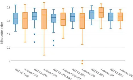
4.3 Analysis of Iterative Seed Expanding Clustering ... 39
4.3.1 Comparing ISEC-V2 vs ISEC... 39
4.3.2 Comparing ISEC-V2 vs I-Adams SRG ... 41
4.3.3 Comparing ISEC-V2 vs Conventional SRG Methods ... 43
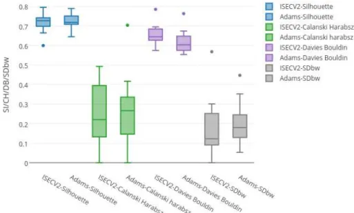
4.4 Fusion Strategy for Unsupervised Clustering Evaluation ... 46
4.4.1 Unsupervised Fusion Analysis of ISEC-V2 vs I-Adams SRG ... 46
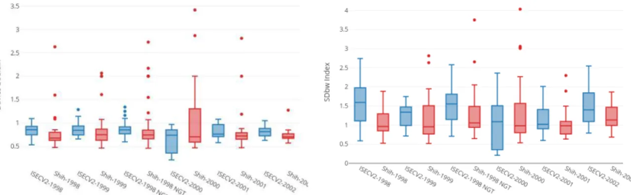
4.4.2 Unsupervised Fusion Analysis of ISEC-V2 vs Conventional SRG Methods ... 48
4.5 Analysis of the Explosion Control in ISEC-V2 ... 51
4.6 Summary of the Results ... 55
5 Conclusion and Future Work... 57
Bibliography ... 58
A The Results ... 62
A.1 Matlab and R Correlation Analysis ... 62
A.2 ISEC-V2 Comparative Results with ISEC ... 63
A.3 SEC vs RSEC Results of F-measure Index ... 64
A.4 Segmentation Results with SST images (Explosion) ... 65
A.5 Segmentation Results with SST images (No Explosion) ... 70
A.6 Segmentation Results with SST images of Canary ... 74
List of Figures
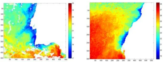
1.1 Applying SEC on SST image, (1.1a) original SST image, (1.1b) corresponding ground truth map, (1.1c) segmentation result by applying the ST-SEC algorithm ... 2 1.2 Applying SEC on SST image, (1.2a) original SST image, (1.2b) corresponding ground truth map, (1.2c) segmentation result by applying the ST-SEC algorithm ... 2 3.1 Resulting images, left one is the segment result from RSEC algorithm and the right one is the result from SEC algorithm ... 25 3.2 F-measure results using SEC and RSEC algorithms for the images of Canary ... 26 3.3 Feature firstmean-min value for sequential extracted clusters on ISEC-V2 ... 28 3.4 ISEC-V2 combine results in terms of F-measures and the number of iterations for images of 1998 and 1999 (Portugal). The left image is the line graph of F-meaure analysis and the right image is the bar chart of number of outer iterations ... 29 3.5 F-measure as a result of Iterative Adams for the images 1998 and 1999 of Portugal. ... 30 3.6 left: the image of Ground-truth, Right: the resulting image from I-Adams ... 31 3.7 Bar chart showing outer iterations comparing ISEC and I-Adams for the images 1998 and 1999 of Portugal. ... 31 3.8 Contour Strength trend for the images of No Explosion 1998-1999 (Portugal)... 33 3.9 Contour Strength trend for the images of No Explosion 1998-1999 (Portugal)... 33 4.1 Two SST images, the left one is from Portugal (1998-07-11) and the right one is from Canary (img_262) ... 36 4.2 Three SST images, the one in the left is the image with strong gradient, the middle one is with weak gradient and the right one is the noisy SST image ... 37 4.3 The ground-Truth of the above image with strong gradient ... 37 4.4 Coordinates of the seeds and the coastline. ... 39 4.5 Silhouette Index analysis comparing ISEC-V2 with I-Adams using the whole data set of SST images (Portugal) ... 41 4.6 Calinski, SDbw and Davies Bouldin indices analysis comparing ISEC-V2 with
4.12 SF-A/SF-G/SF-H/SF-Med fusion measures comparing ISEC-V2 with I-Adams using
the whole dataset of SST images (Portugal) ... 46
4.13 SF-A/SF-G/SF-H/SF-Med fusion measures comparing ISEC-V2 with I-Adams for the images of Canary. ... 47
4.14 SF-A/SF-G/SF-H/SF-Med fusion measures comparing ISEC-V2 with Shih SRG using the whole dataset of SST images (Portugal). ... 48
4.15 SF-A/SF-G/SF-H/SF-Med fusion measures comparing ISEC-V2 with Verma SRG using the whole dataset of SST images (Portugal). ... 49
4.16 SF-A/SF-G/SF-H/SF-Med fusion measures comparing ISEC-V2 with Shih SRG using the images of Canary ... 49
4.17 SF-A/SF-G/SF-H/SF-Med fusion measures comparing ISEC-V2 with Verma SRG using the images of Canary ... 50
4.18 SST images, left image is the original image, middle one is the ground truth and the right image is segmented image with explosion ... 51
4.19 Contour Strength corresponding to the number of iterations, the left image is the one with explosion and the right is without explosion.. ... 52
4.20 Image 19990914 Portugal, Contour Strength with no-explosion ... 52
4.21 First derivative corresponding to the number of iterations of the image 19980612 with explosion ... 53
4.22 Explosion Analysis for the images of 1998-1999, Iterations with actual algorithm and after the CS apply ... 54
4.23 Two SST images, the left one is the ground truth and the right one is the segmented image with explosion ... 55
4.24 First Derivative corresponding to the number of iteration for the image 19980711 (Portugal) ... 55
4.25 Resulting image when RSEC algorithm stops at iteration 51 and ground truth in the background ... 56
A.1 Correlation of Matlab and R using Silhouette index with F-measure ... 62
A.2 Correlation of Matlab and R using Davies Bouldin index with F-measure ... 62
A.3 Correlation of Matlab and R using Calinski Harabsz index with F-measure ... 63
A.4 SST image (1998-06-14) in the left and Ground Truth in the right ... 63
A.5 Segmentation results, left image is the result of ISEC and the right one is the result of ISEC-V2 ... 64
A.6 Iterative result images by ISEC algorithm ... 64
A.7 Iterative result images by ISEC-V2 algorithm... 64
A.8 SST Image 1998-07-15 ... 65
A.9 GT 1998-07-15 ... 65
A.12 Shih-SRG 1998-07-15 ... 66
A.13 Verma-Otsu 1998-07-15 . ... 66
A.14 SST image 1998-07-11. ... 66
A.15 GT 1998-07-11. ... 66
A.16 ISEC-V2 1998-07-11. ... 66
A.17 I-Adams 1998-07-11... ... 66
A.18 Shih SRG 1998-07-11... 67
A.19 Verma-Otsu 1998-07-11. ... 67
A.20 SST image 2002-07-31 ... 67
A.21 ISEC-V2 2002-07-31. ... 67
A.22 I-Adams 2002-07-31. ... 67
A.23 Shih SRG 2002-07-31... 68
A.24 Verma-Otsu 2002-07-31. ... 68
A.25 SST image 1998-06-12 ... ... 68
A.26 GT 1998-06-12. ... 68
A.27 ISEC-V2 1998-06-12. ... 68
A.28 I-Adams 1998-06-12. ... 68
A.29 Shih SRG 1998-06-12... 69
A.30 Verma-Otsu 1998-06-12. ... 69
A.31 SST image 1998-06-14. ... 69
A.32 GT 1998-06-14. ... 69
A.33 ISEC-V2 1998-06-14. ... 69
A.34 I-Adams 1998-06-14 ... 69
A.35 Shih SRG 1998-06-14... 70
A.36 Verma-Otsu 1998-06-14 ... 70
A.37 SST image 1998-08-01 ... 70
A.38 GT 1998-08-01 ... 70
A.39 ISEC-V2 1998-08-01 ... 70
A.40 I-Adams 1998-08-01 ... 70
A.41 Shih SRG 1998-08-01... 71
A.42 Verma-Otsu 1998-08-01 ... 71
A.43 SST image 1998-08-02 ... 71
A.44 GT 1998-08-02 ... 71
A.46 I-Adams 1998-08-02 ... 71
A.47 Shih SRG 1998-08-02 ... 72
A.48 Verma-Otsu 1998-08-02 ... 72
A.49 SST image 1999-09-01 ... 72
A.50 GT 1999-09-01 ... 72
A.51 ISEC-V2 1999-09-01 ... 72
A.52 I-Adams 1999-09-01 ... 72
A.53 Shih SRG 1999-09-01 ... 73
A.54 Verma-Otsu 1999-09-01 ... 73
A.55 SST images 2000-08-08 ... 73
A.56 ISEC-V2 2000-08-08 ... 73
A.57 I-Adams 2000-08-08 ... 73
A.58 Shih SRG 2000-08-08 ... 74
A.59 Verma-Otsu 2000-08-08 ... 74
A.60 SST image 177 ... 74
A.61 GT 177 ... 74
A.62 ISEC-V2 image 177 ... 74
A.63 I-Adams image 177 ... 74
A.64 Shih SRG image 177 ... 75
A.65 Verma-Otsu image 177 ... 75
A.66 SST image 117 ... 75
A.67 GT image 117 ... 75
A.68 ISEC-V2 image 117 ... 75
A.69 I-Adams image 117 ... 75
A.70 Shih SRG image 117 ... 76
A.71 Verma-Otsu image 117 ... 76
A.72 SST image 237 ... 76
A.73 GT image 237 ... 76
A.74 ISEC-V2 image 237 ... 76
A.75 I-Adams image 237 ... 76
A.76 Shih SRG image 237 ... 77
A.77 Verma-Otsu image 237 ... 77
A.78 SST image 1998-06-12 ... 77
A.80 ISEC-V2 1998-06-12 ... 77
A.81 Contour Strength (CS)’s first derivative, 1998-06-12 ... 78
A.82 GT and Segmentation, 1998-06-12 ... 78
A.83 Segmentation at it=37, 1998-06-12 ... 78
A.84 SST image 1998-06-18 ... 78
A.85 GT 1998-06-18 ... 78
A.86 ISEC-V2 1998-06-18 ... 79
A.87 Contour Strength (CS)’s first derivative, 1998-06-18 ... 79
A.88 GT and Segmentation, 1998-06-18 ... 79
A.89 Segmentation at it=49, 1998-06-18 ... 79
List of Tables
3.1 Percentage of improved F-measure using the images of 1998 and 1999. ……..…… 253.2 Images of CANARY island with result of f-measures, using SEC and the new revised version RSEC.………...………...……… 26
4.1 The whole dataset of Portugal and the Canary Island ………...…… 37
4.2 Unsupervised Indices ………...…… 41
4.3 Visual analysis (Explosion and Under-segmentation) for the whole dataset of Portugal and the Canary. ……….……...…… 45
4.4 Fusion Analysis for the whole dataset of Portugal as well as Canary. …...…… 50
I
NTRODUCTION
1.1
Motivation
Upwelling occurred when cold and nutrient–rich water appears over the surface of the ocean by replacing the warm water or nutrient-depleted water. The nutrient-rich water is fertilized that produces a good fishing ground; therefore, upwelling detection is directly related to the maritime economy or blue economy. Due to the presence of cold water in these regions, upwelling areas can be identified by cold Sea Surface Temperatures (SST) and high concentrations of chlorophyll-a. The higher availability of upwelling regions results in high levels of primary fishery production. Roughly, 25% of the total global marine fishing is coming from five different upwelling areas that are 5% of the total oceanic area.
The oceanographers have been using SST images, as described by Nascimento and Franco (2009), and Nascimento et al. (2012), for the identification of conversion zone between the colder and warmer oceanic waters. They applied high scale resolution on SST images, which used to take a lot of time and effort to process one by one. In order to get the best results, a good visualization of the whole phenomena is necessary. The detection and continuous monitoring of upwelling might be an extensive process, therefore, automatic tools are required, because not only a large quantity of data collected daily but also to predict the trend of upwelling areas in different regions and seasons, thus an objective approach to extract that region is necessary.
In the past, different approaches have been adopted in order to perform automatic upwelling detection from SST images. The artificial neural networks were applied to wind and SST data for the prediction of coastal upwelling (Kriebel et al., 1998). Neural network algorithm was used for detection and segmentation of upwelling regions (Chaudhari et al., 2008). The author used k-means clustering results to determine the presence of upwelling. Marcello et al. (2005), based on coarse-segmentation method proposed automatic detection of upwelling. The semi-automated method used for detection of upwelling areas (Plattner et al., 2006). Automatic detection of frontal activity was applied using edge detection algorithm (Nieto et al., 2012). The upwelling extracted by means of Otsu’s automatic thresholding method and Fuzzy C-means (Tamim et al., 2013).
segmentation process, not taking into account the geographical information about the extracted clusters. Moreover, detection of the frontier was entirely separate from the segmentation phase.
Therefore, Nascimento et al. (2015) adapted the Seeded Region Growing (SRG) (Adams and Bischof, 1994) algorithm in order to propose a new algorithm named Seed Expanding Cluster algorithm (SEC). This algorithm not only considered the temperature value of the pixel but also its spatial context in order to combine pixels for segmentation. It grows regions according to the similarity criterion that is, the temperature of the region to the temperature of a seed pixel. The seed pixel is selected in the beginning, which is the pixel with the lowest temperature.
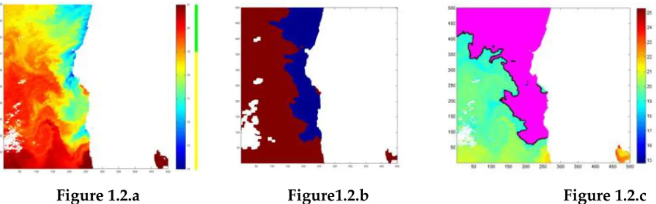
Figure 1.1.a Figure 1.1.b Figure 1.1.c
Figure 1.1: Applying SEC on SST image, (1.1a) original SST image, (1.1b) corresponding ground truth map, (1.1c) segmentation result by applying the ST-SEC algorithm.
The images in this section have been taken from Nascimento et al. (2015), the Figure (1.1.a) is the original image, Figure (1.1.b) is the ground-truth map and Figure (1.1.c) is the resulting image. The SEC algorithm on these images has shown promising results in order to recognize the upwelling area automatically and the frontline. The result with Self-T SEC algorithm is very satisfactory but only in the case of a strong gradient. In the case of smooth gradients explosion has been observed, which can be seen in Figure (1.2.c).
It is difficult to handle upwelling regions with transition zones characterized by smooth gradient boundaries because it is hard to make the distinction between the objects of interest and the background. Segmentation leak or explosion is one of the biggest issues in the detection of upwelling areas.
1.2
Problem Description
The algorithms, which solve the problem of automatic detection of upwelling region, are Seed Expanding Cluster (SEC), Self-tuning Seed Expanding Cluster (ST-SEC) (Nascimento et al., 2015) and the Iterative Seed Expanding Cluster (I-SEC) (Lopes, 2015). All the above-mentioned authors adapted the classical Seeded Region Growing (SRG) algorithm but with different criterion of homogeneity. In SRG, region grows when the homogeneity criterion matches i.e. the difference between testing pixel and the seed pixel. It starts with one pixel or the set of multiple pixels if the objective is to segment multiple areas by adding the similar pixels into the upwelling region according to the homogeneity criteria.
The SEC-algorithm starts with initial seeds but it takes only one pixel to start region growing. The main difference between SEC and SRG is the calculation of homogeneity criterion (threshold) that is, the product of the considering pixels instead of the conventional difference. Therefore, the SEC and its family algorithms (ST-SEC and I-SEC) are different from novel Seeded Region Growing (SRG) in terms of a threshold. In SRG, a threshold is defined manually in order to stop the expansion of growing region, which is not appropriate for automatic detection process, therefore, ST-SEC proposed an automatic calculation method for a threshold. In other versions of SEC, threshold is also calculated automatically from the known clustering automatic threshold methods named Ridler and Calvard (1978); Otsu (1979); Kittler and Illingworth (1986).
1.3
Main Contributions
The main contributions of this dissertation are:
(i) A sequential extraction version of the Seed Expanding Cluster (SEC). This algorithm is composed by two-nested iterative cycles: the inner one responsible for the construction
of the ‘core’ cluster; and the outer one that extracts clusters one-by-one from the residual data. The external stop condition takes advantage of the knowledge domain by defining the seeds selection region and a modeled extracted feature. This new iterative version of SEC Algorithm (I-SECV2) had been experimented on SST images from different regions on the globe having very diverse upwelling patterns;
(ii) The development of an explosion control procedure and its incorporation in the previous algorithm, and the study of the effectiveness of the new version of the
algorithm in avoiding the so‐called leakage problem.
(iii) The development of a sequential extraction version of the benchmark Seeded Region Growing algorithm (Adams and Bischof, 1994), following the architecture of I-SECV2.
(iv) The development of a ‘consensus’ scheme of unsupervised clustering validation measures, since the last explored strategy is far from being satisfactory. Not surprisingly, the obtained results using several validation indices are not concordant between each other. Therefore, it was implemented a scheme of fusion voting for unsupervised validation.
1.4
Organization of the Document
L
ITERATURE
R
EVIEW
2.1
Introduction to Image Segmentation (IS)
Image segmentation is a process of converting an image into partitions called segments. Each segment contains information about color, motion, texture etc. The segments are homogeneous according to some criterion. Image segmentation always plays a leading role in image processing research and it is the first step for image analysis.
The results depend on the way of applying image segmentation methods that means good analysis is directly related to the IS. Mainly there are two objectives of image segmentation, first is to decompose the image into segments and the second is more important i.e., to arrange the pixels into an efficient and meaningful way for further analysis.
It is not a practical approach to process the whole image directly. Therefore, several image segmentation algorithms had been proposed, in the field of image processing before recognition. Image segments classify an image into clusters or regions according to the same features. Now a day, lots of image segmentations algorithm exists and are applied in different fields of science and our daily life. We can categorize these algorithms according to the methods used, like edge-based, region-based and data-clustering based segmentation.
Automate the image segmentation process makes all stages of image processing more efficient and easy. The proposed study is more focused on the clustering automatic threshold for image segmentation that would be discussed in the next section.
Thresholding is one of the simplest methods in IS where pixels are assigned to a category in which the value lies. Each pixel allocated to some category based on a threshold. Furthermore, we have Region-based segmentation in which region grows from one seed or multiple seeds. All of them expand each region pixel by pixel based on the homogeneity criteria. In data clustering, the concept of growing region is based on the distance between each pixel.
2.2
Clustering Automatic Thresholding (CAT) Methods for Image
Segmentation
Thresholding is one of the most popular and widely used methods for image segmentation. The basic idea is to separate foreground from the background by selecting the value for a threshold. This depends on the image features of interest.
Sezgin and Sankur (2004) grouped threshold into six main categories:
1) Histogram-Based, where peaks and valleys of a smooth histogram analyzed. It is also called shaped based methods of thresholding.
2) Clustering based, where grey level samples grouped into two parts, foreground, and the background.
3) Object attribute-based, it includes the methods that measure the similarity between the gray level and the binary image, using fuzzy shape similarity, edge coincidence etc. 4) Entropy-based, analysis features similarity according to the foreground and background
entropy.
5) The spatial-based, methods used higher-order probability distribution and/or correlation between pixels.
6) Local methods, calculate a threshold for each pixel from the local image characteristics. Now we will have a look at three main methods for automatic thresholding of an image that belongs to above discussed clustering-based methods.
Ridler and Calvard’s method
Otsu’s method
Kittler and Illingworth’s method
Formulation
:Let the pixels of an image represented in terms of L gray levels . The number of pixels at level is denoted by and the total number of pixels by . The gray-level histogram normalized and the probability distribution is:
. (2.1)
Now assume that the pixels divided into two classes background and foreground, and threshold at level ; background denotes pixels with levels and foreground denotes pixels with levels .
, (2.2)
. (2.3)
, (2.4)
, (2.6)
. (2.7)
2.2.1
Ridler and Calvard’s method
Ridler and Calvard (1978) proposed an iterative process for an image thresholding method. In this method, an optimal value of threshold has chosen automatically because of an iterative process. Iterations provide a cleaner extraction of the object region. They introduce a signal controlling function in which if the function received zero value, the image will signal the background and vice versa.
The switching function (threshold) is defined as the average of the foreground and background class means.
(2.8)
The process starts by reading the image pixel by pixel. It stops when the switching function remains constant for further iterations.
Selection of an optimal threshold is very difficult to achieve therefore this method proposed maximum four iterations.
2.2.2 Otsu’s method
According to Otsu (1979), automatic selection of threshold is based on unsupervised and nonparametric method. It assumes that the image contains two classes of pixels following bi-modal histogram (foreground and background), then it calculates the optimum threshold mathematically by separating classes in a way that their combined intra-class variance is minimal, or equal to their inter-class variance is maximal.
The total variance is the sum of the within-class variances and the between-class variances.
(2.9)
where “ ” is the probablity of backgroud class and foreground class respectively.
2.2.3
Kittler and Illingworth’s method
The method proposed by Kittler and Illingworth (1986), starts by calculating the bi-model histogram of the grey level image h(g) then it estimates the prior probability P of the calculated histogram. In the end, the mean is equal to the total probability.
It is the initial Threshold of the given image and separates the image into classes foreground and background.
Kittler proposed the criterion function:
(2.10)
and the desired threshold is based on the minimization of criterion function that is:
(2.11)
2.3 Seeded Region Growing (SRG) Methods for Image Segmentation
2.3.1
Adam’s Seeded Region Growing Method
Adam and Bishof (1994) proposed a region-growing algorithm called SRG, which is widely used in a different kind of application nowadays. The SRG is based on the conventional region growing assumption, that is, region grows based on similarity of pixels. It is a simple and robust method for growing region systematically. The good results can be achieved in the first step but it majorly depends upon the selection of seeds, therefore, high-level knowledge of image is the root of selection seeds.
It starts with placing the initial seeds in the image, where each seed could be a single pixel or set of pixels. Regions grow with these pixels by adding neighboring pixels to them who qualify the criterion. The SRG stops when all the pixels have allocated some region (only one).
Mainly SRG based on two factors: 1) The seed selection, and
2) The similarity criterion
The homogeneity or similarity criterion is defined as the difference between the testing pixel and the pixel of interesting region R.
where is the gray value of the pixel . Main issues with SRG are:
1) To start the algorithm, how to select a good initial seed? 2) What is the threshold for the region to grow?
3) How to manage the labeling of the pixels?
2.3.2 Adaptive Seeded Region Growing using Automatic Thresholding
Seeded Region Growing (SRG) is a fast and robust method for image segmentation and has the ability to adapt other techniques to make the process more efficient. In this section, we will discuss the adaptive SRG using homogeneity criterion (threshold) more automatic.
2.3.2.1 Linear SRG and Quadratic SRG
Linear and Quadratic SRG algorithm by Fan and Lee (2015), relaxed the grey level assumption of the original SRG. Since the SRG (original) does not impose any restriction on the growing regions, therefore it would produce very rough segmentation boundaries. They also introduced a stabilized SRG that encourages smoother boundaries and prevents the so-called leakage or explosion problem.
In SRG, similarity criterion is assumes that the grey value of any region does not change and can be a single constant value. Linear SRG relaxes this assumption by modeling the grey values with linear plane.
Let the numbers of rows and columns of an image be and , and the coordinates of a pixel located at that point are respectively. The new Linear SRG method is modeled as
where are coefficients of the corresponding plane, and ε is error term, usually assumed to be identically and independently distributed. The new homogeneity criterion based on linearity is:
(2.13)
Quadratic SRG is similar to the Linear SRG but the only difference is that it is modeled in quadratic planes. The homogeneity criterion in this contrast is:
(2.14)
2.3.2.2 Seed Expanding Cluster (SEC)
The single-seeded region-growing algorithm by Nascimento et al. (2015) was inspired by SRG (classical model) but with different homogeneity criterion in the format of a product. The growth is controlled by a similarity threshold and it stops when no more pixels remain in the frontier boundary. We will discuss SEC algorithm and its versions in detail in section 3.
2.3.2.3 The Verma Seeded Region Growing
Verma et al. (2011) proposed a single-seeded region growing method similar to the SEC algorithm for color image segmentation. The algorithm starts from the central pixel of the image as seed. It grows only one region at a time and in order to tune the automatic threshold value, it uses Otsu’s adaptive thresholding technique.
The similarity criterion is based on the intensity of the pixels, that is:
(2.15)
where is the intensity value of the testing pixel N , and is the intensity value of the seed. The value is the threshold that derived from Otsu’s method of automatic thresholding to grow cluster.
2.3.2.4 The Shih and Cheng Seeded Region Growing
Shih and Cheng (2005) proposed an automatic seed region-growing algorithm derived from the classical SRG (Adams and Bischof, 1994). It starts with more than two seeds to grow the regions. It resolves the problem of seed selection in classical SRG by introducing an automatic selection of initial seeds. For automatic seed selection, three criteria must be satisfied.
1) Seed pixel must have high similarity to its neighbors. 2) At least on seed is selected from expected region. 3) Seeds from different regions must be disconnected.
The homogeneity criterion in order to combines regions is defined by:
(2.16)
2.3.2.5 The Zanaty and Asaad Seeded Region Growing
This method called a probabilistic Region Growing because it was based on the probability of the pixels. The algorithm presented by Zanaty and Asaad (2013) depends on the different homogeneity criterion. It starts the growth with the seed pixel and stops when pixel does not match the homogeneity criterion. The pixels that pass the criteria move from the frontier F to the cluster C.
(2.17)
where F and is the mean intensity of the pixels in the cluster C. The pixel assigned to the cluster C if it passes the following similarity criterion:
(2.18)
where is the intensity of the testing pixel and is the probability of that intensity value. It calculated the threshold dynamically by:
(2.19)
2.4
Domains of Application
In past, great scientific work had done where Seeded Region Growing used to solve the complex problems. Due to simplicity and robustness of SRG algorithm, now days, it has been used in different domains with conjunction of other algorithms.
2.4.1 SRG in Industrial Application
SRG used in many industrial applications at different domains. Lachance et al. (2004) presented a region growing technique to measure the wear flat area through grinding machine. The process controls automatically the position of the wheel and captures digital images of the wheel between grinding cycles. Pottmann et al. (2005) used SRG for the problems of geometric optimization in Geometry applications. Zhengtao (2011) proposed Capsule Image Segmentation Based on Linear Region Growing by analyzing the traditional image segmentation method SRG. Hadwiger et al. (2008) presented a novel method for interactive exploration of industrial CT volumes such as cast metal parts, with the goal of interactively detecting, classifying, and quantifying features using a visualization-driven approach.
2.4.2 SRG in Medical Image Processing
In the field of Medical Image Processing, Seeded Region Growing algorithm is used for the detection of tumor and also used in brain MRI. Stokking et al. (2000) applied SRG to brain MRI images to visualize and quantify the segments. The method is called morphology-based brain segmentation. As the brain, tissues are very connected to each other so other algorithms are also used with SRG in order to find good results. Pohle and Toennies (2001) presented a new self-learning, fully automatic region-growing segmentation of medical images.
Mat-Isa et al. (2005) applied SRG on digital images and called the method a Seeded Region Growing Feature Extraction. This method used to extract the size of the nucleus, size of cytoplasm, grey level of nucleus and grey level of cytoplasm. Wong and Zrimec (2006) presented a novel technique, which uses a seeded region-growing algorithm to guide the
classifier to regions with potential honeycombing. The classification used for analyzing the
patterns of lung diseases. Chen et al. (2006) proposed a sketch-based interface for seeded region growing volume segmentation. A user freely sketches regions of interest (ROI) directly over the 3D volume. Parts of the volume outside the ROIs are then automatically cut out in real-time.
Wang and Chen (2012) established Automatic Vector Seeded Region Growing for Parenchyma Classification in Brain MRI. Nuclear magnetic resonance (NMR) can be used to measure the nuclear spin density, the interactions of the nuclei with their surrounding molecular environment and those between close nuclei, respectively. Al-Faris et al. (2013) used a system with automated features for MRI breast tumor segmentation.
2.4.3 SRG in Remote Sensing
applied to segment images, which are being used to assess land use changes in the Amazon region. Bagli et al. (2004) presented Automatic delineation of shoreline and lake boundaries from Land sat satellite images. Gao et al. (2011) established different segmentation methods in multispectral Landsat images to achieve object based image classification, and used SRG as one of the method. Wang and Chen (2012) proposed an hybrid algorithm that contains different steps including clustering k-means, segment initialization, seed generation, region growing, and region merging. The algorithm used widely in remote sensing data, and also used in urban and regional planning. Stroppiana et al. (2012) introduced a method for extracting burned areas from landsat images using some techniques, which include a region-growing algorithm. Zhang et al. (2013) extracted coastline in aquaculture zones by using region growing segmentation with multiple steps. Mishra and Susaki (2013) proposed some methodologies based on the analysis of multi-temporal Synthetic Aperture Radar images.
2.5
Strategies for Controlling Explosion in SRG
In the process of region growing, the original classical method (SRG) does not impose shape restriction on the contour (boundary) of the region. When there is a weak gradient between the target and the neighbor region, the results could have a very large size of the region and also could have very rough boundaries. In addition, the so-called Leakage or the explosion problem could occur. This leakage problem refers to the situation when the grey values of targeted and the neighbor objects are very similar, and the growing region of one object breaks the true boundary and enters to the other object’s region.
We are going to explore different strategies in this section, which controls the explosion in adaptive SRG methods.
2.5.1 Stabilized Seeded Region Growing
Fan et al. (2014) proposed a variant of SRG as discussed in section (2.3.2.1), that encourages smoother boundaries and the aim is to prevent the explosion problem. During the growth process, Stabilized-SRG not only considers the grey value of x, but it also takes into account the grey values of neighboring pixels. This set of neighboring pixels are denoted by the square of size (2L+1) * (2L+1) centered as x.
The neighboring pixels define as:
where (2.20)
The parameter L determines the smoothness of the boundary. Larger the value of L smoother will be the boundary. In practice, it can be chosen by a user (operator) in an attractive manner, moreover prior knowledge about the image is necessary.
2.5.2 New Region Growing Based on Selection of Optimal Threshold and Seeds
Afifi and Ghoniemy (2015) proposed an algorithm that works with local search process to achieve the optimal threshold and better seed selection. The output seeds are the input of local search algorithm to extract the best seeds around initial seeds. Seed selection and get optimum threshold overcomes the limitations of classical SRG as described in section (2.3.1). The algorithm works automatically that means it works without any predefined parameters.
In both histogram-based and region-based segmentation techniques, if the threshold is not correct or not optimum, the contour of the object will destroy and causes an explosion. The algorithm hybridized the seed selection, local search, and thresholding algorithms with the region growing technique in order to get good segmentation results.
It iteratively merges similar pixels into regions in 3 main steps: 1- Choice of the seed pixels;
2- Local search according to a similarity rule;
3- Thresholding algorithm for growing the regions by including adjacent pixels that satisfy the similarity rule.
The Proposed method resolved the issue of optimum threshold of SRG by using the homogeneity test where RA is the seed pixel. The seed pixel has maximum amplitude from grey level histogram.
The author defines the thresholding algorithm as follows:
The image is divided into two parts using initial threshold T old. The average grey level values for each part (mean1, mean2) is computed then updates threshold value by:
and stop when the condition |<delta satisfied.
Where delta = .
2.5.3 Leak Detection using Distance Transformation in SRG
This method used region grower tool that is, a user defines seed then the segmentation starts and regions grow while neighboring pixels lie within a specific grey value range. This works very well when the segmented image contrast is good but when the contrast is not sufficient at the contour the algorithm produces leaks. This is because of similar grey values of the targeted region and the neighborhood. Often the origin of the leak is only a narrow connection between the boundaries of targeted and neighbor pixels.
This method used Distance Transformation technique in order to identify the leak regions and then remove that additional area from the segmentation. The basic idea was to calculate the path from a random point within the erroneous area to the seed point, which supposed to maintain the maximum possible distance. The bottleneck is the point whose local maximum has the shortest distance hence the origin of the leak. For every pixel, repeat the same process then search the two nearest, opposing points on the contour and separate the segmented area along a line between these two points. The part of the area where the user clicked is then removed from the segmentation.
2.5.4 Automatic Detection by gradient magnitude likelihood classification and
Correction of Segmentation Leaks
Kronman et al. (2011) proposed a method that identifies the segmentation leak basis boundary by gradient magnitude likelihood classification. The leak basis boundary then fits the surface and leaks has been removed from the targeted structure by finding the common boundary.
Segmentation leaks are one of the most invasive segmentation errors that can be found in any algorithm. According to the author, leaks produce in the segmentation when the pixels gradient intensity magnitudes of the target and neighboring region boundaries are too small or the characteristics are very similar. After the leaks are found the most important task is to remove them from the results, therefore extensive manual user interaction is required. Many prior shape knowledge-based models have been proposed in order to reduce segmentation leaks. These models have drawbacks as they are structure specific, relies on the experts (manual intervention) and are time-consuming because of the prior generation of the shape.
Heimann et al. (2004) introduced a method, as described in section 2.5.3 that explicitly detects a segmentation leak by computing a path by shortest distance procedure between two user-defined points but this method automatically detects and corrects leaks. The method first finds out the leak basis boundary then fits a surface to pixels of this boundary. The leak is then separated from the target structure by re-labeling the leak basis pixels as background. Since the leak is the actual boundary between targeted and the neighbor structure, so the goal is to find the segmentation leak basis.
The leak L between the target structure T and a neighbor structure N is a set of pixels in I that are classified by ST.
(2.21)
where S is the set of structures of interest. If there is no leak.
The leak detection is consists of 4 steps.
1- 2-
3- 4-
There are some major advantages of this method.
It is independent of the segmentation method used;
It does not require any prior shape, location and/or intensity information; It is fully automatic;
After the identification of LBB the correction could be achieved by eliminating the leaks. For each segmentation leak L, it re-labels the leak basis pixels as background and finds the target-connected component.
2.6 Clustering Validation Approaches
2.6.1 Supervised vs. Unsupervised Evaluation
Image segmentation is the first important step in many multimedia applications. In this area, many different approaches and algorithms were proposed, but no one guaranteed to get the best results. To address this problem evaluation criterion was used to quantify the quality of the results since last few years. Supervised evaluation is the one in which user assistants is involved that means it needs some prior knowledge (ground-truth) required by experts to compare the results. Whereas in unsupervised evaluation no user assistant is required whereas some statistics are computed from the segmentation result.
Evaluation methods that require user assistance, are infeasible in many computer vision applications, so unsupervised methods are necessary.
The very well known measure that was used in supervised evaluation is F-measure (Rijsbergen, 1979). It combines precision and recalls then calculate the values from confusion matrix and cross-validate the results with the ground-truth. Precision is the proportion of predicted positive cases that are correctly real positives, while recall is the proportion of real positive cases that are correctly predicted positive. F-measure gives the value range from 0 to 1, the highest value shows better results we get. The second most important measure is Adjusted Rand Index (ARI), presented by Hubert and Arabie (1985) that was based on the similarity between two data clusters. ARI can score from negative values to 1 and the highest value means good results. In this study, we will use the F-measure as supervised evaluation for the experimental results.
2.6.2 Unsupervised Validation Measures
In external validation, one can use external information not present in the data but when we do not have this information then internal validation is used. Internal validation relies on the information inside data. Data characteristics like noise, monotonicity, density etc. are the basic information that is used for the internal validation indices.
Internal validation takes into account the compactness and the separation of the clusters. How closely the objects are in the cluster is compactness and it is based on variance. Lower variance means high compactness of the clusters. The separation is about how clusters are well separated to each other.
Internal validation process starts by applying the clustering algorithm to the data set. Each clustering algorithm then uses different combinations of parameters to get different clustering results. Now compute internal validation index of each partition or cluster. The best partition has the optimum cluster number.
One of the most important challenges in data clustering now days is how to evaluate the results without auxiliary information. Esendira et al. (2011) address this problem by comparing different internal validation indices. As the internal indices depend upon the intrinsic information present in the data so, the results can be different for different type of data.
According to Liu (2010), S-Dbw is one of the best indices between other unsupervised indices but the data he used was very simple in nature. Chouikhi (2015) compared 30 different internal indices and found that CH and DB perform the best.
Below we have some of the most popular validation indices those are included in the proposed study.
2.6.2.1 Calinski-Harabasz index
(2.22)
where is the between-cluster scatter matrix, is the within-cluster scatter matrix, is the number of cluster points and is the number of clusters. Maximal value of indicates that the results are good.
The index evaluates the results based on the average between- and within-cluster sum of squares.
2.6.2.2 Dunn index
The Dunn validity index (Dunn, 1974), sometime called distance ratio index because it takes into Account the min and max distances between two points.
(2.23)
where is the minimum distance between two points belonging to different clusters, and
is the maximum distance between any two points selected from the same cluster. The
maximal value of will indicates better candidate.
The index uses the minimum pair wise distance between objects in different clusters as the inter-cluster separation and the maximum diameter among all clusters as the intra-cluster compactness.
where and are the weights.
2.6.2.3 Davies-Bouldin index
This internal validation index, proposed by Davies and Bouldin (1979), used to evaluate the clustering results. It is based on the similarities of the obtained clusters.
(2.24)
The index is calculated for each cluster C as, compute the similarities between C and all other clusters, and the highest value is assigned to C as its cluster similarity. Then index can be obtained by averaging all the cluster similarities. The smaller value of the index shows good results.
2.6.2.4 Silhouette index
Rousseeuw (1987), proposed the Silhouette index in order to validates the clustering results based on the pair wise difference of between and within-cluster distances as:
(2.25)
where k is the number of clusters. is the number of objects in ith cluster. Moreover, the optimal value of the index shows best results.
2.6.2.5 S_Dbw Validity Index
Halkidi et al. (2001) proposed a new clustering validity index based on density.
(2.26)
where is the inter-cluster separation and is the intra-cluster density.
E
XTENDING THE
S
EED
E
XPANDING
C
LUSTERING AND
R
ELATED
M
ETHODS
3.1
The Seed Expanding Cluster (SEC) Method and its Algorithms
The Seed Expanding Clustering algorithm (SEC) (Nascimento et al., 2015) is a new algorithm extending the Seeded Region Growing (SRG) by defining a homogeneity criterion inspired on the concept of approximate clustering (Mirkin, 1996). The approach differs in that the algorithm thresholding values are not expert-driven but rather derived from the approximate clustering model.
The algorithm starts from a pixel with the lowest temperature value in the SST map and uses it as the initial seed. Then, it grows a region by labeling the boundary pixels and expanding simultaneously. This method resolves the problem of boundary pixels labeling and the dependency of pixel sorting order, therefore the SEC algorithm performs these in parallel to speed up the procedure.
The algorithm can be summarized as follows: it receives temperature map T(R, L) as an input where R is the set of rows and L the set of columns and elements of R × L are pixels.
Step 1: In the first step pre-processing stage, the data is normalized by taking each pixel in the image and subtract it from the average temperature.
Step 2: The second step of the algorithm is the Cluster Initialization, each pixel with the exploring window centered at the seed pixel go into the cluster if homogeneity criterion satisfies.
(3.1)
where is the temperature of the seed pixel, is the temperature of tested pixel and is the temperature similarity threshold.
Step 3: Set Cluster Boundary is the third step in which a set F is define as:
(3.2)
where is the set of 8-neighborhood pixels.
In SEC, the homogeneity criterion comprises by two separate conditions, the temperature similarity and the density condition. The temperature similarity condition, equation (3.3), makes SEC different from the conventional SRG and ensures that the expansion of the cluster is smooth with the temperature variation, and the density condition equation (3.4), covers a continuous fragment of the ocean.
(3.3)
where the temperature define as and representing the current boundary pixel temperature.
The density condition is defined as the total number of pixels those are in the cluster and intersect the exploring window , divided by the number of total pixels in the window :
(3.4)
where is the density threshold and if both of the conditions satisfy then that pixel is enter into the cluster.
The major innovation of the algorithm is its similarity criterion (3.3.) that takes the form of a product rather than a difference as in SRG algorithms. The Self-tuning version of the algorithm (ST-SEC) dynamically calculates the threshold values, directly derived from the clustering criterion (Nascimento et al., 2015), (Nascimento and Mirkin, 2017). Its value changes depending on the state of the cluster C and its interception with the window .
The ST-SEC is similar in structure to the other version of the algorithm, except the calculation of threshold value π that define as:
(3.5)
There were developed distinct versions of the SEC algorithm according to the adopted method to calculate the threshold values. Specifically: SEC-Otsu (Nascimento et al., 2015),the method used in this version is the one derived from Otsu (1979). In SEC- Kittler, and SEC- Ridler (Lopes, 2015), the threshold is calculated from Kittler and Illingworth (1986), and Ridler and Calvard (1978) respectively.
3.2
The Iterative Seed Expanding Cluster (ISEC) Algorithm
The upwelling area sometime appears in different coastal regions. The SEC algorithm only grows one region because it takes only one seed; however, for tackling the problem of extracting the multiple upwelling areas, it is necessary to run the region growing procedure more than once. An iterative version of the SEC algorithm (I-SEC) was developed and experimentally studied by Lopes (2015) in his master thesis, had to treat the problem of discontinuous upwelling areas.
The proposed iterative SEC (ISEC-V2) modifies the stop condition of the previous ISEC in order to enhance the efficacy and efficiency of the algorithm. The ISEC-V2 stop condition comprises of two sub-conditions.
C1: Coastline distance calculation is the first stop condition, in which the selected seed distance is calculated from the coastline if the seed is far from the coastline the algorithm stops. How the coastline and the distance are calculated will be described in section (4.3.1). This removes completely the stop condition in the previous algorithm where the iterations were fixed to five.
3.3
Improved Iterative Seed Expanding Clustering Algorithm
The ISEC algorithm comprises inner and outer stop conditions. The inner stop condition is related to the SEC algorithm as described in section (3.1), the algorithm for the core cluster formation. The outer stop condition ISEC stop condition itself and responsible for the formation of more than one upwelling areas.
3.3.1 Inner Stop Condition: the Revised SEC
The revised SEC algorithm is the same as described in section (3.1) in structure but we made few changes in order to increase the effectiveness of the segmentation results. In addition, we had compared the results with SEC method and found the results with improvements. The original SEC algorithm has been revised in the following aspects:
i) The neighborhood to explore the cluster boundary, F (equation (3.2)) was set to a window of 4-neighborhood instead of 8-neighborhood;
ii) It was adopted a pixel-to-pixel update of the cluster during the dilatation of the boundary F;
iii) The inner stop condition is defined by the stability of the cluster, substituting the condition of the empty boundary.
Figure 3.1: Resulting images, left one is the segment result from RSEC algorithm and the right one is the result from SEC algorithm.
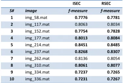
We took 30 SST images of 1998 and 31 of 1999 from Portugal and also 10 images from Canary island. We applied SEC and RSEC for this data set and observed that with our new revised version (RSEC) the F-measure improved to some extent.
Table 3.1: Percentage of improved F-measure using the images of 1998 and 1999.
R-SEC
SEC
R-SEC
85%
SEC
15%
Table 3.2: Images of CANARY island with result of f-measures, using SEC and the new revised version RSEC.
ISEC RSEC
S# image f-measure f-measure
1 img_58.mat 0.7776 0.7781
2 img_117.mat 0.8063 0.8034
3 img_152.mat 0.7754 0.7828
4 img_177.mat 0.8013 0.8084
5 img_214.mat 0.8451 0.8485
6 img_237.mat 0.8268 0.8307
7 img_262.mat 0.8136 0.8054
8 img_310.mat 0.8061 0.8077
9 img_334.mat 0.7237 0.7265
10 img_336.mat 0.7231 0.7267
Figure 3.2: F-measure results using SEC and RSEC algorithms for the images of Canary.
3.3.2
Outer Stop Condition: the Revised ISEC
The ISEC algorithm resolved the problem of discontinuity but had the problem of complexity of the algorithm due to the several stop conditions as described in section (3.2). The algorithm contains inner and outer stop conditions. The inner stop condition is related to the revised SEC algorithm as described in section (3.3.1), the algorithm for the core cluster formation. The outer stop condition is related to ISEC and is responsible for the formation of more than one upwelling areas. In this section, we will discuss the revision of outer stop condition in ISEC to form a new iterative version named Iterative Seed Expanding Cluster (ISEC-V2) and will compare the results with the previous ISEC version.
The ISEC-V2 took advantage of the domain knowledge that seeds exist near the coast because the water is coolest in that area. The revised version ISEC-V2 calculates the coastline and records the coordinates and the spatial values of each coastline pixel.
The coastline once calculated at the start of the algorithm and took these coordinates in the iterative process for the distance calculation between the seed and the coastline pixel at that position. The coastline formation will be discussed in detail in section (4.3.1); the formation of coastline is the base of ISEC-V2 because this revised version main stop condition is related to the coastline. If the seed exists near the coastline, that seed would be the mature seed and take into consideration but if not then the algorithm will stop. The distance is calculated with respect to the coastline coordinates.
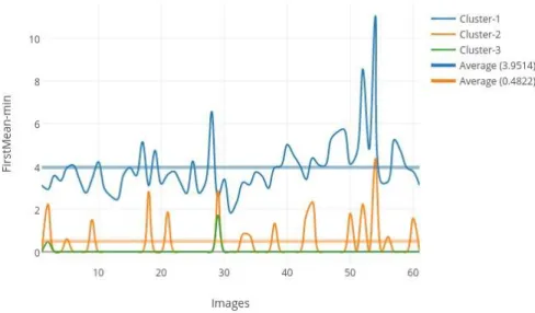
Figure 3.3: Feature firstmean – min value for sequential extracted clusters on ISEC-V2 algorithm.
We tested the approach with two subsets of SST images for the upwelling seasons of 1998 and 1999 for this calculation as shown in figure (3.3), and found that for the first cluster, the average value was 3.9 and it decreased to 0.48 an average in the second cluster. Hence, we used Otsu, to calculate the good threshold value, in our experimental study instead of the fixed threshold.
The ISEC-V2 showed promising results in terms of segmentation and the efficiency. We did experiments with ISEC-V2 for the images of 1998 and 1999 and found that the f-measure remains stable and the execution time to process each image decreased because of a number of iterations of the outer loop.
Figure 3.4: ISEC-V2 combine results in term of F-measures and the number of iterations for images of 1998 and 1999 (Portugal). The left image is the line graph of F-measure analysis and the right image is the bar chart of number of outer iterations
3.4
Sequential Iterative Version of Adams SRG (I-Adams)
Adams and Bischof (1994) proposed an SRG method that based on the similarity of the pixels in order to grow the region as described in section (2.3.1). The Adams SRG is simple and continues being an extensively used SRG algorithm. The similarity criterion of Adams is; the difference of the testing pixel and the pixel of an interested region as mentioned in equation (2.12).
The first main drawback or the problem of Adams was the selection of the initial seed or seeds because it based on the single seed as well as multiple seeds. The second problem of Adams was to identify the number of regions that means it does not found that how many clusters are in the data. Hence, to overcome these problems we developed an iterative version of Adam's SRG, homologous to ISEC-V2: sequentially extracting clusters one by one from the residual SST map until the stop condition holds. This version is called, I-Adam SRG.
The seed selection in ISEC-V2 is the pixel near the coastline as described in section (3.3.2) that removed the problem of seed selection in Adams. Moreover, the iterative version resolved the second problem i.e., how many regions or clusters are in the data.
Figure 3.5: F-measure as a result of Iterative I-Adams for the images 1998 and 1999 of Portugal.
Figure 3.6: left: the image of Ground-truth, Right: the resulting image from I-Adams
Figure 3.7: Bar chart showing outer iterations comparing ISEC and I-Adams for the images 1998 and 1999 of Portugal.
Thefigure (3.7) shows the efficiency of new I-Adams in terms of the total number of outer iterations. The previous iterative model was fixed the iteration to five whereas in new
3.5
Proposed Strategy for Explosion Control
It is well known that region-based segmentation algorithm suffers from the problem of an explosion, also denoted as leaking problem. In intensity-based thresholding and region-growing methods, they appear when the pixels intensity of the leak boundaries and inside the target structure is very close. In adaptive region growing methods, like SEC they appear when the intensity distribution of the leak and the target structure are similar.
In this section, we are going to introduce a strategy for explosion control and will implement in conjunction with SEC algorithm to cope up the problem of leakage (explosion).
3.5.1 The Contour Strength (CS) Criterion
We choose the contour strength (CS) measure, adapted from the literature (Siebert, 1997), as the measure to detect explosion in the expanding process of the clusters. The reason for the selection of this strategy in my proposed work is that it introduces a very good measure for the quality of growing region by maximizes the contour strength
The contour strength of a region R is the sum of the absolute differences between each pixel on the contour and the neighbor of contour points that do not belong to the region of interest, i.e.
(3.6)
where is the set of pixels on the contour of R.
The general idea is that regions are bounded by strong contour, therefore regions grow such as to maximize We assumed the strategy that the cluster expands by maximizing its contour strength.
We calculate the CS as mentioned in equation (3.6), by taking the difference of the pixel on contour (boundary (F)) and the neighbors those do not belong to the cluster. We tested CS on all those images of 1998 and 1999, which had an explosion and all those, where explosion did not appear. The detail experimental results will be discussed in section (4.5), where we will also examine the CS in conjunction with RSEC. The study has been done systematically because getting good results were not possible in one-step. We first calculate the first derivative of the CS of cluster R and analyze the trend of its values for the SEC segmentations facing explosion as opposed to the ones without explosion. We observed that few images not shown good results as expected i.e. the images with no explosion shows downward slope (weak CS). To cope up the problem we used the concept of Moving Average will be discussed in detail in section (4.5) so that we can get the smooth boundary.
Figure 3.8: Contour Strength trend for the images with Explosion 1998-1999 (Portugal).
Figure 3.9: Contour Strength trend for the images with No Explosion 1998-1999 (Portugal).
3.6
Fusion Strategy for Unsupervised Clustering Validation
As discussed in Section (2.6.3), it is well known that internal validation indices are not concordant among them, therefore; we decide to introduce a fusion procedure in which all the unsupervised indices as mentioned in section (2.6.3) are used separately. In this section, we will discuss those fusion indices and the results we got from them.
3.6.1 Fusion method for Clustering Validity Indices (CVI)
We explored a fusion approach for clustering validation adapted from Kryszczuk and Hurley (2010). The method called fusion because it calculates the index based on the multiple unsupervised indices. In the proposed study, we will use this method by using the normalized data of Silhouette index, Davies Bouldin index, Calinski-Harabasz index and S_Dbw index as described in section (2.6.2).
Silhouette index normally ranges from 0 to 1. The Davies Bouldin is considering being good when it has a lower index and it normally ranges from 0 to 2. The S_Dbw is similar to the Davies Bouldin that means lower index value considering being good. The Calinski Harabasz is different from all three indices because its value ranges from 0 to any whole number. Its goodness depends upon the higher value of the index. As the values range is diversified for the different indices, so for the fusion we normalized the data ((value – min)/max) to keep its range from 0 to 1. The goodness of fusion indices depends on the higher score value. This method comprises four different fusion measures named as SF-A, SF-G, SF-H, and SF-Med.
(3.7)
where is the number of indices used and represents the index. As mentioned above we used four unsupervised indices with their normalized values therefore, this index takes the sum of these values (SI + DB + CH + SDbw) and divided by 4.
(3.8)
where is the number of indices used and represents the index. This fusion index uses product (SI x DB x CH x SDbw) instead of the sum as in above index and take the root with value 4, as 4 is the total number of indices we used. The higher value of the index shows goodness of the results.
(3.9)
where is the number of indices and represents the index. It takes reciprocal of each unsupervised index value (1/SI + 1/DB + 1/CH + 1/SDbw) and sum up them. In the last, this term is divided with total number of unsupervised indices i.e. 4.
(3.10)
E
XPERIMENTAL
S
TUDY
4.1
Goals of the Study
The main goals of the experimental study are:
(i) To analyze the effectiveness of the new Iterative SEC algorithm, ISEC-V2, comparing it against the previous one, as well as with the proposed Iterative Adam’s SRG algorithm I-Adams SRG;
(ii) To experimentally fine-tune the parameters of the strategy to control the explosion problem on SRG, incorporate it in the ISEC-V2, and experimentally analyze the effectiveness of the algorithm in preventing the leakage problem;
(iii) To develop a fusion strategy of internal clustering validation indices to perform the unsupervised evaluation of the segmentation results;