João Pedro Mateus Gens dos Santos
Licenciatura em Ciências de Engenharia BiomédicaBrain circuits involved in self-paced motion:
the influence of 0.1 Hz waves
Dissertação para obtenção do Grau de Mestre em Engenharia Biomédica
Orientador: Alexandre Andrade,Doutor,
Instituto de Biofísica e Engenharia Biomédica,
Faculdade de Ciências da Universidade de Lisboa
Júri:
Brain circuits involved in self-paced motion: the influence of 0.1 Hz waves
Copyright cJoão Pedro Mateus Gens dos Santos, Faculdade de Ciências e Tecnologia, Universidade Nova de Lisboa
A
CKNOWLEDGEMENTS
First of all, I would like to express my sincere gratitude to my supervisor, Alexandre An-drade. This dissertation wouldn’t have been possible without his introduction, guidance, useful comments, remarks and encouragement. I am very grateful for his example and testimony. He will be no doubt a reference in my life. Thank you very much!
My sincere thanks goes to the Technical University of Graz for kindly made available all the subjects datasets used on this work and, particularly, to Gert Pfurtscheller’s group to discuss the results with me. A special thank to Joana Brito and João Rodrigues for introduce me to this project and clarify me all my doubts on the beginning of this dissertation. Your help was very important and is part of this dissertation.
I would like to thank all the professors at FCT-UNL who have gave me the scientific basis necessary to develop this project, in particular all the professors of Biomedical Engi-neering. I would also like to thank the Institute of Biophysics and Biomedical Engineering (IBEB), where this dissertation was conducted, for all the support provided during this time.
I wish to thank all my colleagues and friends of the FCT-UNL who have accompanied me during these last years. You are all different and special and I wish you all the best for the future. Thanks for all the help during these years. I would also like to thank my friends and colleagues I met during this project in IBEB, who have accompanied me and shared with me very valuable moments. You guys are amazing people! Thank you very much.
I would like to thank all the people of my hometown, that made me grow, and all the friends and colleagues that I have known. Thank you very much.
A
BSTRACT
The neural mechanisms behind human voluntary motion are not fully characterized yet, in spite of numerous research studies. Slow ( 0.1 Hz) brain oscillations are known to have a powerful modulatory effect on several cognitive and physiological phenomena, including free movement.
This study is based on fMRI data acquired from 25 young, healthy subjects. The tasks were: rest, self-paced motion, motion paced by a periodic 0.1 Hz stimulus. The temporal resolution was finer than standard fMRI protocols (TR=871 ms). After preprocessing, the signal from brain regions of interest was extracted, and functional connectivity was com-puted between brain regions using wavelet phase coherence. Complementarily, effective connectivity was measured using Granger causality. The final output was Phase-Locking (PL) and Granger Causality (GC) matrices reflecting inter-regional phase coherence and causal interactions, respectively, around 0.1 Hz.
Using the GraphVar toolbox, inter-task and inter-group comparisons were performed. In inter-task comparisons PL matrices showed encouraging results unlike GC matrices. Pairs of regions for which PL differs significantly between rest and self-paced movement were identified. These include mainly the Postcentral gyrus, Putamen, the Anterior Cin-gulum, the Precentral gyrus, the Calcarine, the Lingual and the Insula (all in the left hemisphere). Topological changes in the brain wiring were identified across the tasks by computing the node degree and global efficiency. Inter-group comparisons took into account the inter movement interval and the coupling between BOLD and heart rate beat-to-beat interval signals and showed changes in brain activity depending on the regularity of movement intervals and specific connectivity patterns for neural BOLD oscillations, respectively.
This methodological approach allowed to make a contribution towards the characteri-zation of the functional connectivity of brain circuits related to voluntary motor behavior.
R
ESUMO
Os mecanismos neuronais que estão por detrás das ações voluntárias humanas ainda não estão inteiramente caracterizados, apesar dos numerosos estudos realizados. As oscilações cerebrais lentas são conhecidas por terem um poderoso efeito modulatório em vários fenómenos cognitivos e fisiológicos, incluindo o movimento livre.
Este estudo é baseado em dados de fMRI adquiridos de 25 sujeitos jovens e saudáveis. As tarefas foram: repouso, movimento espontâneo e movimento regulado por um estimulo periódico de 0.1 Hz. A resolução temporal usada foi superior à da maioria dos protocolos de fMRI usados correntemente (TR = 871 ms). Depois do pré-processamento, o sinal das regiões cerebrais de interesse foi extraído e a conectividade funcional foi calculada entre regiões cerebrais usando a coerência de fase baseada em wavelets. Complementarmente, foi medida a conetividade efetiva usando a causalidade de Granger. O resultado final foram matrizes de coerência de fase e causalidade de Granger refletindo coerências de fase inter-regionais e interações causais, respetivamente, ao redor de frequências de 0.1 Hz.
Usando o software GraphVar, comparações inter-tarefa e inter-grupo foram realizadas. Para as comparações inter-tarefa, as matrizes de coerência de fase mostraram resultados encorajadores ao contrário das matrizes de causalidade de Granger. Pares de regiões para os quais a coerência de fase difere significativamente entre repouso e movimento espontâneo autónomo foram identificados. Incluídas estão principalmente regiões da cir-cunvolução Pós-central, Putâmen, Cíngulo Anterior, circir-cunvolução Pré-central, Calcarino, Lingual, e a Insula (todos no hemisfério esquerdo). Alterações topológicas nas redes de conectividade cerebrais foram identificadas ao longo das tarefas através do cálculo do grau do nó e eficiência global. Comparações inter-grupos tiveram em conta o intervalo entre movimentos e a relação entre o sinal BOLD e o intervalo entre picos R do sinal cardíaco registado em simultâneo e mostraram alterações na atividade cerebral dependendo da regularidade dos intervalos dos movimentos e padrões específicos de conetividade para as oscilações neuronais BOLD, respetivamente.
Esta abordagem metodológica deu um contributo para a caracterização da conetivi-dade funcional dos circuitos cerebrais relacionados com o movimentos voluntário espon-tâneo.
C
ONTENTS
Contents xi
List of Figures xiii
List of Tables xvii
1 Introduction 1
1.1 Objectives . . . 2
1.2 Dissertation overview . . . 3
2 Background 5 2.1 Voluntary movements . . . 5
2.1.1 Brain circuits . . . 6
2.1.2 Slow oscillations . . . 6
2.2 Magnetic Resonance Imaging . . . 8
2.2.1 functional Magnetic Resonance Imaging . . . 9
2.3 Brain connectivity . . . 11
2.3.1 Brain networks . . . 12
2.3.2 Topological measures of brain networks . . . 14
2.3.3 Measures of neuronal signal synchrony . . . 17
2.3.3.1 Cross-correlation . . . 17
2.3.3.2 Cross-coherence . . . 17
2.3.3.3 Phase Synchronization . . . 19
2.3.3.4 Granger Causality . . . 19
3 Materials and Methods 23 3.1 Participants, Image acquisition and data pre-processing . . . 23
3.2 Methodology 1 . . . 24
3.2.1 Wavelet Coherence Analysis - Phase Locking . . . 24
3.2.2 Statistical Test - Length of significant Phase Locking segments . . . 27
3.3 Methodology 2 . . . 27
3.3.1 Granger Causality Analysis . . . 28
3.4 GraphVar toolbox - comprehensive graph analysis . . . 29
3.4.1.1 Raw connectivity matrix . . . 30
3.4.1.2 Network construction and calculation . . . 31
3.4.1.3 Statistical analysis . . . 32
3.4.2 GraphVar - Methods . . . 32
3.4.2.1 Networks Nodes / Brain areas. . . 33
3.4.2.2 Inter-task comparison . . . 36
3.4.2.3 Inter-group comparison. . . 37
4 Results and Discussion 39 4.1 GraphVar - Exploration of Results . . . 39
4.2 Phase Locking and Granger Causality - Relationship. . . 40
4.3 Inter-task and inter-group comparisons . . . 41
4.3.1 Inter-task comparison . . . 41
4.3.1.1 Mean PL matrices - 14 Brain Regions . . . 41
4.3.1.2 Time length of significant phase locking matrices - 14 Brain Regions . . . 46
4.3.1.3 Granger Causality - 14 Brain Regions . . . 46
4.3.1.4 Mean PL matrices - 24 Brain Regions . . . 49
4.3.1.5 Mean PL matrices - Network Calculations . . . 50
4.3.2 Inter-group comparison . . . 57
4.3.2.1 Inter-movement interval . . . 57
4.3.2.2 Anxiety/STADI scales. . . 58
4.3.2.3 BOLD-RR Interval . . . 59
5 Conclusions 65 5.1 Future Work . . . 67
5.2 Contributions . . . 67
Bibliography 69
A Poster 79
L
IST OF
F
IGURES
2.1 Brain circuits for voluntary action. a | Left-hand panel: The primary motor
cortex (M1) receives a key input from the SMA and the preSMA, which in turn receives inputs from the basal ganglia and the prefrontal cortex. Right-hand panel: information from early sensory cortices (S1) is relayed to intermediate-level representations in the parietal cortex, and from there to the lateral part of the premotor cortex, which projects in turn to M1. b | Brain activity pre-ceding a voluntary action of the right hand. The frontopolar cortex (shown in green) forms and deliberates long-range plans and intentions. The pre-SMA (shown in red) begins the preparation of the action with other premotor areas generating the readiness potentials (red trace) that can be recorded from the scalp. Immediately before the action takes place, M1 (shown in blue) becomes active. In later stages of preparation the contralateral hemisphere is more ac-tive than the ipsilateral hemisphere; this is reflected in a lateralized difference between the readiness potentials that are recorded over the two hemispheres of the brain (solid and dotted blue traces). Finally, neural signals leave M1 for the spinal cord and the contralateral hand muscles. The contraction of the muscles is measured as an electrical signal, the electromyogram. Adapted from (Haggard, 2008) . . . 7
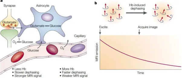
2.2 Upon activation, oxygen is extracted by the cells, thereby increasing the level of deoxyhaemoglobin in the blood. This is compensated for by an increase in blood flow in the vicinity of the active cells, leading to a increase in oxy-haemoglobin. An increase in the concentration of deoxyhaemoglobin would cause a decrease in image intensity, and a decrease in deoxyhaemoglobin would
cause an increase in image intensity. Adapted from Heeger and Ress (2002) . 11
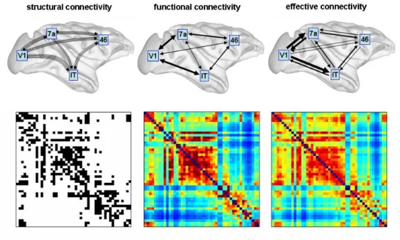
2.3 Examples of different types of brain connectivity networks and respective
adja-cency matrices. Adapted fromhttp://www.scholarpedia.org/article/
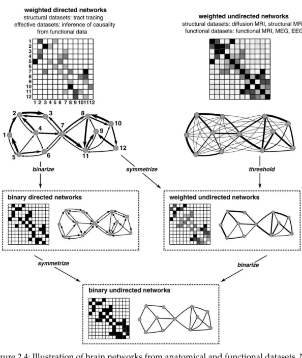
2.4 Illustration of brain networks from anatomical and functional datasets. Net-works are commonly represented by their connectivity matrices, with rows and columns representing nodes and matrix entries representing links. To sim-plify analysis, networks are often reduced to a sparse binary undirected form, through thresholding, binarizing, and symmetrizing. Adapted from (Rubinov and Sporns, 2010) . . . 15
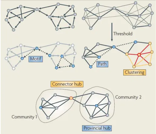
2.5 The figure shows a schematic diagram of a brain network drawn as a direct(left) and an undirected (right) graph as well as different structures such as nodes, links, a hub, motif, the representation of clustering, communities and Paths. Adapted from (Bullmore and Sporns, 2009) . . . 16
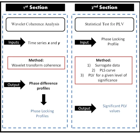
3.1 Analysis scheme for the two main sections of the methodology. The first section is based on Wavelet Coherence computation for time series x and y extracted from the ROIs of interest. The outputs from this step are the phase difference profiles from which the phase locking profiles are obtained. In the second section a statistical test is performed for phase-locking values (PLV) using the output from the first step as input to this section. A surrogate approach is applied followed by computation of the PLV values of surrogate pairs (Phase-Locking Statistics=PLS) and identification of PLV values (from the first section) above a user-defined significance level. Adapted from (Brito, 2014) . . . 25
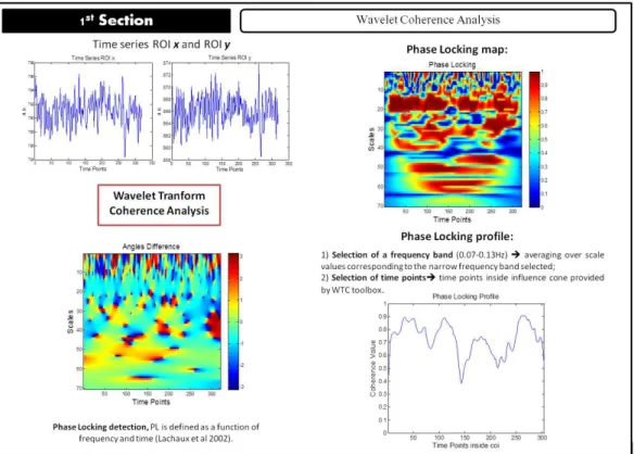
3.2 Analysis scheme for the first section. From WTC the Angle/Phase differences
maps over all time points and scales (time-frequency analysis) are obtained, followed by computation of the locking map. In order to obtain phase-locking profiles, a frequency band is selected (in this example: 0.07−0.13Hz) and the values corresponding to the selected frequencies are averaged and plotted as a function of time. Points outside the cone of influence are excluded. Adapted from (Brito, 2014) . . . 26
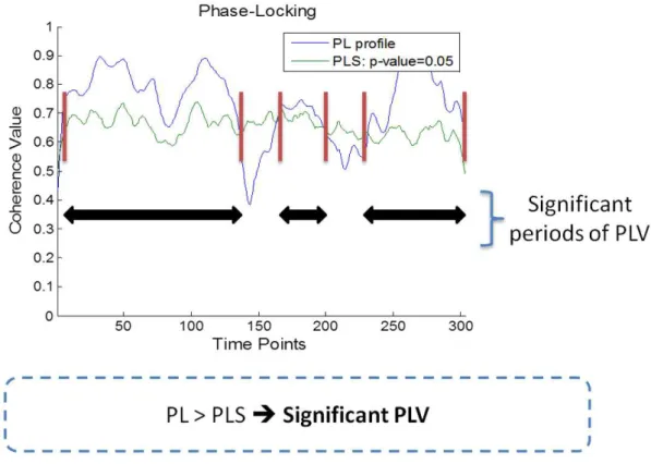
3.3 Phase-locking analysis. In blue: Phase-locking (PL) profile for a sample pair of ROI signals. In green: Phase-Locking Statistics (PLS) curve corresponding to p<0.05. Adapted from (Brito, 2014) . . . 28
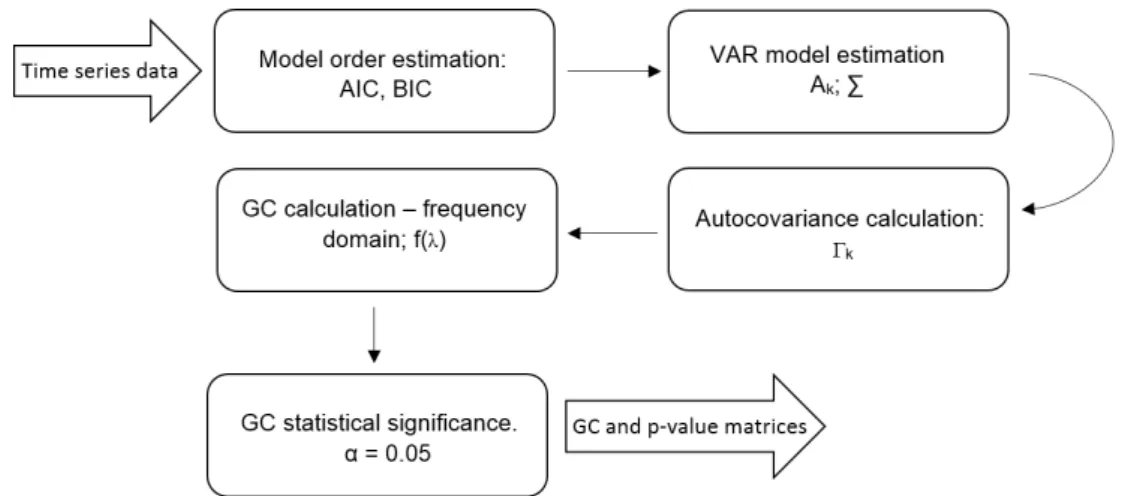
3.4 Schematic of the computational process followed with the MVGC Toolbox
(Seth and Barnett, 2014) . . . 29
3.5 Schematic workflow of GraphVar. Adapted from (Kruschwitz et al., 2015) . . 30
3.6 GraphVar setup interface. Adapted from (Kruschwitz et al., 2015) . . . 33
3.7 Schematic depicting the methods followed with GraphVar. Matrices containing
LIST OFFIGURES
4.1 GraphVar interactive results viewer . . . 40
4.2 Scatter plots containing information about the PL and GC, where GC is from
region Supplementary motor area to Insula. All the 25 participants were con-sidered . . . 42
4.3 Scatter plots containing information about the PL and GC, where GC is from
region Insula to Supplementary motor area. All the 25 participants were con-sidered . . . 43
4.4 Inter-task comparison involving the four tasks performed by participants, two resting sessions and two movement sessions. Matrices containing information about Phase Locking were used. . . 45
4.5 Inter-task comparison involving the four tasks performed by participants, two resting sessions and two movement sessions. Matrices containing information about time length of significant Phase Locking were used. . . 47
4.6 Inter-task comparison involving the four tasks performed by participants, two resting sessions and two movement sessions. Matrices measuring Granger Causality were used . . . 48
4.7 Inter-task comparison involving the four tasks performed by participants, two resting sessions and two movement sessions.(a),(b) and (c),(d) show Rest > Self contrast regarding the acquisition a and b, respectively. Matrices containing information about Phase Locking were used. . . 50
4.8 Inter-task comparisons considering the node degree measure. The contrasts
Rest1 > Rest2, Rest1 > Self and Rest1 > Visual are shown. The values 0.1, 0.2, 0.3, 0.4 and 0.5 represent the relative thresholds applied to create the networks. Only the brain regions that p-values were significant are shown. . . 52
4.9 Inter-task comparisons considering the node degree measure. The contrasts
Rest2 > Rest1, Rest2 > Self and Rest2 > Visual are shown. The values 0.1, 0.2, 0.3, 0.4 and 0.5 represent the relative thresholds applied to create the networks. Only the brain regions that p-values were significant are shown. . . 53
4.10 Inter-task comparisons considering the node degree measure. The contrasts Self > Rest1, Self > Rest2 and Self > Visual are shown. The values 0.1, 0.2, 0.3, 0.4 and 0.5 represent the relative thresholds applied to create the networks. Only the brain regions that p-values were significant are shown. . . 54
4.11 Inter-task comparisons considering the node degree measure. The contrasts Visual > Rest1, Visual > Rest2 and Visual > Self are shown. The values 0.1, 0.2, 0.3, 0.4 and 0.5 represent the relative thresholds applied to create the networks. Only the brain regions that p-values were significant are shown. . . 55
4.13 Inter-task comparisons considering the global efficiency measure. The values 0.1, 0.2, 0.3, 0.4 and 0.5 represent the relative thresholds applied to create the
networks. Only the brain regions that p-values were significant are shown.. . 57
4.15 Acquisition b; Inter-group comparison based on the inter movement interval of the participants when executing self paced motion. . . 59
4.16 Acquisition a; Inter-group comparison based on Anxiety scales of the partici-pants in the first resting state. . . 60
4.17 Acquisition a; Inter-group comparison based on Anxiety scales of the partici-pants in the second resting state. Non-significant results to A > B . . . 60
4.18 Acquisition b; Inter-group comparison based on Anxiety scales of the partici-pants in the first resting state. Non-significant results to A > B . . . 60
4.19 Acquisition b; Inter-group comparison based on Anxiety scales of the partici-pants in the second resting state. . . 61
4.20 Acquisition a; Inter-group comparison based on BOLD RR Interval of partici-pants in the first resting state. . . 62
4.21 Acquisition a; Inter-group comparison based on BOLD RR Interval of the participants in the second resting state.. . . 62
4.22 Acquisition b; Inter-group comparison based on BOLD RR Interval of the participants in the first resting state. . . 62
L
IST OF
T
ABLES
A
CRONYMS
BOLD Bold Oxygen Level Dependent.
EEG Electroencephalography.
fMRI functional Magnetic Resonance Imaging.
GC Granger Causality.
M1 Primary Motor Cortex.
MEG Magnetoencephalography.
MRI Magnetic Resonance Imaging.
PET Positron Emission Tomography.
PL Phase Locking.
SMA Supplementary Motor Area.
C
H
A
P
T
E
R
1
I
NTRODUCTION
The impression that one can freely choose between different possible courses of action is fundamental to human life. This capacity has long been a topic of debate first for theologians and philosophers and nowadays also for psychologists and neuroscientists. The fundamental question is: are we completely defined by the deterministic nature of physical laws or do we have some independence in making choices and actions? A dualistic view is present in our normal language and suggests that the mental state "I" that is distinct from both brain and body, freely initiate the neural events in motor areas of the brain that lead to body movement. However, modern brain science has suggested that this subjective experience of freedom is no more than an illusion and that our actions are initiated by unconscious mental processes long before we become aware of our intention to act (Haggard,2005).
Voluntary movements have been generally assumed to be a result from neural activity in premotor and motor cortical areas that precede the conscious decision to move. Studies in which subjects freely choose between moving the right of left hand showed activation of medial frontal cortex. In particular, regions such as supplementary motor area and anterior cingulate cortex are involved. Brass and Haggard(2010a)hypothesize the involvement of anterior insular cortex in evaluating the outcomes of intentional action decisions that are previously formed elsewhere (Brass and Haggard,2010a).
for instances, the so called Mayer waves (Julien,2006). This has lead researches to hy-pothesize that the intention to perform a motor act could be dependent on cardiovascular oscillations (Pfurtscheller et al.,2012b).
fMRI has played a prominent role in the quest to identify the brain regions involved in voluntary action. This technique has enabled researchers to visualize changes in brain activity noninvasively. Bold Oxygen Level Dependent (BOLD) technique has been the most employed fMRI method. It is based on changes in the ration of oxy-to deoxyhemoglobin which consequently causes changes in the magnetic resonance signal. This technique has given support to the comprehension of how different parts of the brain are functionally organized (Huettel et al.,2004).
Functional organization of the brain has been characterized by segregation of local areas and their global integration during perception and behaviour. These functional interactions occur with synchronized activity between multiple local and distant brain regions and can be mapped in different networks: anatomical network, functional network, effective network. These represent patterns of anatomical links, of statistical dependencies, or of causal interactions, respectively. Normally, networks are formalized as a mathemati-cal object consisting of a set of nodes and a set of links between the nodes. These can be quantitatively described by a set of local and global measures that characterize structural and functional regularities (Sporns,2013).
To estimate functional relationships between two brain regions, different measures of synchrony have been applied. Among them are the wavelet phase coherence and Granger Causality (GC). The former is a practical method for the direct quantification of frequency-specific synchronization (i.e phase locking) between two neuroeletric signals. The latter identifies direct functional ("causal") interactions between two neuroeletric signals (Lachaux et al.,1999; Seth et al.,2015).
1.1
Objectives
Understanding the human brain is one of the most greatest challenges facing the 21st century science. The reasons are mostly because we still know little about the brain’s complexity and because there are still many brain disorders like Alzheimer’s, Schizophre-nia, Autism, Epilepsy or traumatic brain injury that are incurable. Recently, several brain research initiatives have arisen all over the world such as the U.S. BRAIN initiative, the Europe’s Human Brain Project or the Japan’s Brain/MINDS. These projects aims to map the brain in a unprecedented detail, in terms of activity and anatomy and to develop theoretical neuroscience to make sense of it.
1.2. DISSERTATION OVERVIEW
provides a measure of Phase Locking (PL) which has been associated to neural communi-cations. Moreover, it allows to assess the statistical significance of PL values by mean of a surrogate-based statistical test.
Additionally, a complementary method based on the work developed by Seth et al.(2015)is followed. This aims to measure effective connectivity among different brain regions to the same specific frequency band according to Granger causality formulation. This method is based on multiple equivalent representations of a VAR model by regression parameters, the auto-covariance sequence and the cross power spectral density.
At last, this project aims to apply a new tool for network analysis, the "GraphVar", which allows one to do group and inter group comparisons of subjects and construct, characterize, and to do statistics on network topological measures (Kruschwitz et al.,2015).
1.2
Dissertation overview
The remainder of this dissertation is organized as described in this section.
Chapter 2 reviews the background literature related to the work developed in this dissertation. In particular, it provides lights on voluntary actions, their brain circuits and ongoing oscillation underpinning these actions, overviews the functional magnetic reso-nance imaging technique, and comes within the concept of brain connectivity, introducing brain networks, their types and topological measures, as well as a detailed explanation of some measures of signal synchrony relevant to this project.
Chapter 3 details the relevant materials for this study and explains the methodology followed in this project.
Chapter 4 summarizes the key results that show brain networks involved in self-paced motion.
C
H
A
P
T
E
R
2
B
ACKGROUND
2.1
Voluntary movements
It is difficult to explain what makes a particular action voluntary. One of the most common ways to conceptualize voluntary action in cognitive neuroscience has been to contrast it with stimulus-driven actions (Goldberg,1985). This distinction is based on the notion that action strongly guided by the environment are experienced as less volitional. For instances, the reflexes are immediate motor responses determined by stimulus which do not leave much space for volition. Considering this perspective, a voluntary action is defined as internally guided behaviour wherein the occurrence, timing and form are not directly determined. This conception of intentional action is quite controversial because the internally guided behaviour is difficult to define operationally since internal causes of behaviour are not experimentally tractable (Nachevemail and Husain,2010; Schüür and Haggard,2011). However a large number of studies have considered this conception and progress has been achieved.
a key feature of voluntary action (Haggard,2008).
To better understand voluntary action it is worth comparing them with reflex actions. Voluntary action involves the cerebral cortex, whereas some reflexes are purely spinal. Volition has a late maturation in individual development, whereas reflexes can be pre-sented at or before birth. Finally, voluntary action involves the subjective experiences of "intention" and "agency" which are absent in reflexes. "Intention" is related to planning to do or being about to do something and the experience of "agency" is the later feeling that one’s action caused a external event (Haggard,2005).
2.1.1 Brain circuits
Several distinct cortical motor circuits that contribute to voluntary action have been identified in the human brain (Fig.2.1). These circuits converge on the Primary Motor Cortex (M1) which executes motor commands by transmitting them to the spinal cord and muscles (Haggard,2008). The first circuit (FIG. 2.1a) starts with the input from the basal ganglia to the Supplementary Motor Area (SMA) which is thought to play the major part in the initiation of action. This linkage is based on studies of patients with Parkinson’s disease which show less frequent and slower actions than healthy controls (Jahanshahi et al.,1995) and recordings from scalp electrodes that detected a signal of a forthcoming voluntary response, 2 seconds before the movement onset (Loukasa and Browna,2004). Then, the input reaches the preSMA which forms part of a wider frontal cognitive-motor network that includes the premotor, the cingulate and the frontopolar cortices (Dum and Strick, 2005). Several neuroimaging studies have shown the strong activation of preSMA for self-paced actions (Deiber et al., 1999; Jenkins et al., 2000). Moreover, the role of the preSMA is confirmed by recordings from scalp electrodes, which show a prolonged and increasing negativity, the so called "readiness potential", that begins 1s or more before the onset of voluntary movement and which its early part has been localized in the preSMA (Shibasaki and Hallett,2006). Finally, and as a result of the onset of the readiness potential (FIG. 2.1b), neural activity spreads from the preSMA back to SMA and M1, thus causing movement. The second circuit (FIG. 2.1a), starts in the early sensory cortices that relays the information to intermediate -level representations in the parietal lobe and thence to the lateral part of the premotor cortex, which projects in turn to M1 (Rizzolatti and Gd Luppino,1998). This circuit plays a part in immediate sensory guidance of actions, however it also contributes to some aspects of voluntary behaviour. Thus, when a immediate action is required, the parietal- premotor circuit might arbitrate between action alternatives whereas, in the absence of immediate instruction, the basal ganglia-preSMA circuit might be more involved in initiation actions (Haggard,2008).
2.1.2 Slow oscillations
2.1. VOLUNTARY MOVEMENTS
oscillations with periods of minutes to very fast oscillations with frequencies reaching 600 Hz. Slower oscillations, or fluctuations have been detected in the brain when this is at rest and include the frequencies between 0.01 and 0.5 Hz. (Someren et al.,2011). In this dissertation the term slow oscillation is attributed to oscillations in the band frequency of 0.01-0.1Hz.
The slow oscillations were first detected in local field potentials recordings from the rabbit neocortex (Aladjalova,1957) but have since been observed in several other mam-mals (Filippov and Frolov,2004; Filippov et al.,2007; Leopold et al.,2003) and are readily detectable in full band Electroencephalography (EEG) recordings from humans (Vanhatalo et al.,2004). They have been detected during sleep by several EEG methods (Achermann and Borbély, 1997; Nir et al.,2008) but their role in physiology of sleep is still poorly understood. It is believed that this very slow oscillations are well suited to coordinate activity across large corticocortical networks (Buzsaki,2006) and that they could, in this way organize sleep-dependent neuroplastic processes such as the consolidation of episodic memory. In addition, these fluctuations have been shown influence the precipitation of certain types of epileptic seizures (Vanhatalo et al.,2004).
Fluctuations in brain activity below 0.1 Hz have also been observed in the BOLD fMRI signal (Biswal et al.,1995). These oscillations have evidenced correlated regions in the mo-tor cortex and in other neuroanatomical systems including visual (Cordes et al.,2000; Lowe et al.,1998), auditory (Cordes et al.,2000), memory (Vincent et al.,2006), language (Hamp-son et al.,2002) and the most prominent, the default – mode network (Fransson,2005).
In addition, slow arterial blood pressure, heart rate, oxygen availability of cortical tissue, cerebral blood-flow velocity, oxyhemoglobin changes and cerebrospinal fluid have shown oscillations around 0.1 Hz (Taga et al.,2000; Toronov et al.,2007; Tzeng et al.,2010; Vanhatalo et al.,2004; Zhang et al.,1998; Zheng et al.,2010). In particular, arterial blood pressure oscillations, the so called Mayer waves have evidenced a significant correlation with oscillations of sympathetic nerve activity. Studies have shown that these waves are not simply a surrogate of sympathetic nerve activity but they undoubtedly reflect the sympa-thetic response to perturbations in the overall baroreceptor –vascular system (Julien,2006). However, the origin of these waves is still unknown.
The intriguing possibility that the slow oscillations may influence brain responses and other brain activities seems increasingly likely. It has been hypothesized that these oscillations reflect the excitability dynamics of cortical networks (Pfurtscheller et al.,2011). In particular, it has been investigated if these oscillations can be related to the intention to perform a motor act (Pfurtscheller et al.,2012a; Pfurtscheller et al.,2012b; Pfurtscheller et al.,2014a; Pfurtscheller et al.,2011).
2.2
Magnetic Resonance Imaging
2.2. MAGNETIC RESONANCE IMAGING
atomic nuclei magnetic proprieties, in particular, those of the hydrogen atoms.
Hydrogen atoms are constituted by a single proton and are used in MRI due both to their magnetic proprieties and abundance in the human body. They can be seen as positively charged spheres that are spinning around their axis giving rise to a magnetic moment along the direction of the axis of the spins. This magnetic field is the source of the signal that is to be measured. In the absence of an external magnetic field the nuclei are randomly oriented and therefore do not give rise to a magnetic moment. In contrast, when placed into a strong magnetic field the nuclei stay align with the field creating a magnetization in the direction of the field. While aligned the nuclei precess about the field with an angular frequency determined by the Larmor frequency, but at a random phase with respect to one another.
In order to measure the magnetization of the nuclei one must perturb the equilibrium and "excite" the nuclei with a radiofrequency pulse. Radiofrequency causes the nuclei to absorb energy at a particular band frequency aligning their phases and tipping them over the transversal plane. With this pulse the longitudinal magnetization decreases and a new magnetization is established. After the radiofrequency pulse is removed, the system return to equilibrium disappearing the transversal magnetization (transversal relaxation) and growing back the longitudinal magnetization(longitudinal relaxation). The energy released is the signal that can be measure with a receiver coil.
The longitudinal relaxation is seen as an exponential recovery in magnetization de-scribed by time constantT1and transversal relaxation is seen as an exponential decay in
magnetization described by a time constantT2caused by loss of phase coherence of the
nuclei. These both times change from tissue to tissue providing the creation of MR images with a complete distinction between different tissue types. The termT2∗is similar toT2but
also consider the local inhomogeneities in the magnetic field created by changes in blood flow and oxygenation. In this case the nuclei de-phase quicker than they normally would. TheT2∗time underlies the fMRI technique as it detect neurovascular changes which follow psychological and behavioural functions.
2.2.1 functional Magnetic Resonance Imaging
functional Magnetic Resonance Imaging (fMRI) is a neuroimaging technique used to mea-sure the hemodynamic response of the brain in relation to the neural activities. Basically, it measures changes in blood oxygenation and blood flow related to neuronal activity, providing the means to study human brain function in vivo, either in response to certain task or when at rest.
is paramagnetic and hence forms local microscopic magnetic field gradients increasing proton dephasing. Neural activity is supported by a haemodynamic response in the local vasculature. This response leads to an increase in cerebral blood flow to the active region. This served to satisfy an increase in the rate of oxygen and glucose metabolism by increasing the delivery of these substrates. In practice the haemodynamic response oversupplies the active region with oxygenated blood, increasing blood oxygenation down-stream of the arteriole in the capillaries and veins. This reduces the concentration of paramagnetic deoxyhaemoglobin and hence reduces susceptibility induced dephasing. In turn this increases the relaxation timeT2∗. Thus,T2∗ weighted images are what enables fMRI to measures changes of oxygenation in the blood: a lower signal implies a higher concentration of deoxygenated haemoglobin than oxygenated haemoglobin while a higher signal implies a higher concentration of oxygenated haemoglobin than deoxygenated haemoglobin. Because neural activity elicits a substantial supply of oxygenated blood, a increase in signal in the correspondent voxel is expected, and this signal is the BOLD time-series (Filippi,2009).
fMRI benefits of high spatial resolution compared with many other functional imag-ing modalities, such as Positron Emission Tomography (PET), Magnetoencephalography (MEG) and EEG. For humans studies it is on the order of 27-36mm3. It has limiting factors such as the signal strength and the point-spread function of BOLD imaging, which typi-cally extends beyond the actual neural activation sites into draining veins. Regarding data analysis, some choices limit the spatial resolution. For instances, spatially smoothing fMRI data prior to analysis leads to a decrease in the effective resolution of the data. Another issue is alignment of the individual brains through a registration or wrapping process which introduces substantial blurring and noise in a group average and limits the spacial resolution. However, advances in data aquisition and preprocessing can improve space resolution. For example, the use of multiple coils with different spacial sensitivities (paral-lel imaging) or the introduction of enhanced spatial inter-subject normalization techniques to avoid the most dramatic effects of blurring the data, respectively (deCharms,2008), can be applied.
2.3. BRAIN CONNECTIVITY
Figure 2.2: Upon activation, oxygen is extracted by the cells, thereby increasing the level of deoxyhaemoglobin in the blood. This is compensated for by an increase in blood flow in the vicinity of the active cells, leading to a increase in oxyhaemoglobin. An increase in the concentration of deoxyhaemoglobin would cause a decrease in image intensity, and a decrease in deoxyhaemoglobin would cause an increase in image intensity. Adapted from Heeger and Ress(2002)
the order of hundreds milliseconds. Recent technological developments designated by "simultaneous multi-slice" MRI, have sped up the temporal resolution by approximately an order of magnitude (from 2s to 0.2 s) and appear to offer the possibility to be faster (Faro and Mohamed,2006).
2.3
Brain connectivity
refutation of functional localization as a complete explanation of cortical organization in favor of functional specialization and integration as a more plausible theory. Nowadays, the understanding of the brain functioning follows these two principles of functional organization with connectivity as a mediator.
The functional organization of the brain has been characterized by principles of segre-gation of specialized neurons and brain areas, often organized into distinct neuronal pop-ulations, and integration between independent neuronal populations (Tononi et al.,1994). Lachaux et al.(1999)hypothesised the possibility that such integration could be mediated by neuronal groups, oscillating on specific narrow frequency bands, entering into a specific phase-locking over a limit period of time. Some years before, Roelfsema et al.(1997) re-ported evidence for long-range synchronizations between widely separated brain regions which was in accordance the notion that phase synchronization should subserve overall integration of all dimension cognitive acts, including associative memory, emotional tone and motor planning. Fries(2005)hypothesised that neural communication is mechanis-tically subserved by neural coherence, in other words the communication is due to a pattern of phase-locking among oscillations in the communicating neural groups. This was called "communication-through-coherence" (CTC) hypothesis and it is based on the fact that activated neuronal groups have the intrinsic property to oscillate and that those oscillations constitute rhythmic modulations in neuronal excitability that affects both the likelihood of spike output and the sensitivity to synaptic input. Thus, only coherence oscillating (or phase-locked) neuronal groups can communicate effectively, because their communication windows for input and for output are open at the same times (Fries,2005).
2.3.1 Brain networks
A network (or graph) is a mathematical model of a real-world complex system and is defined by a collection of nodes (or vertices) and links (or connections) between pairs of nodes (Rubinov and Sporns, 2010). Nodes in large-scale brain networks usually repre-sent brain regions, while links reprerepre-sent anatomical, functional or effective connections. Normally, the networks are represented by their connectivity (adjacency) matrices where rows and columns denotes the nodes and matrix entries denotes links. Figure (2.3) shows illustrative anatomical, functional and effective connectivity networks.
2.3. BRAIN CONNECTIVITY
Figure 2.3: Examples of different types of brain connectivity networks and respective adja-cency matrices. Adapted fromhttp://www.scholarpedia.org/article/Brain_ connectivity.
Functional connectivity networks:are expressed as statistical dependences between pat-terns of gray matter activity and thus does not necessarily reflect direct neural interactions along synaptic paths. Statistical dependences may be estimated by measuring cross-correlation, spectral coherence or mutual information from time series observation. Time series data may be derived with a variety of techniques, including EEG, MEG and fMRI. Functional connectivity is highly time-dependent exhibiting non-stationary fluctuations even with techniques that operate with a slow sampling rate such as fMRI.
Effective connectivity networks:describe the influence one neuronal system exerts upon another and provides directed networks that represent causal interactions between acti-vated brain areas. It is not "model free" and requires the specification of a causal model including structural parameters. Experimentally, effective connectivity can be inferred through perturbations, or through the observation of the temporal ordering of neural events.
small blocks of tissue represent each node. These parcellation schemes should completely cover the surface of the cortex, or of the entire brain, and individual nodes should not spatially overlap. Furthermore, as parcellation schemes may differ in their proprieties it should be used the same parcellation schemes in the network construction so that these could be compared.
Links can also be differentiated on the basis of their weight and directionality (Fig.2.4). Binary links denote the presence or absence of connections and weighted links contain information about connection strength. Weights in anatomical networks may represent the size, density, or coherence of anatomical tracts, while weights in functional and effective networks may represent respective magnitudes of correlation or causal interactions. Binary networks are in most cases simpler to characterize comparing to the weighted although weighted characterization usually focuses on different aspects of networks organization and may be useful in filtering the non-significant links. The weak and non-significant links tend to obscure the topology of strong and significant connections and when applying an absolute or weighted threshold are normally discarded. Usually, thresholds values are arbitrary determined and the networks should be characterized across a broad range of thresholds. Another characteristic of the link is that they can have directionality. Thus, effective connections can be represented with direct links (Sporns,2011).
2.3.2 Topological measures of brain networks
Brain networks can be quantitatively described by a wide variety of measures. These variously detect aspects of functional integration and segregation, quantify importance of individual brain regions and characterize patterns of local anatomical circuitry. Network measures can be represented as measures of individual networks elements (nodes and links) which typically quantify connectivity profiles associated with these elements and hence reflect the way in which they are embedded in the network, or a measure of all individual elements providing a more global description of the network (i.e normally characterized by its mean). In addition, network measures also have binary and weighted, direct and undirected variants (Sporns,2011).
• Node Degree:measures the number of links connected to the node. Connection weights are ignored in calculations;
• Strength:is the sum of weights of links connected to the node;
• Clustering coefficient:defined locally as the fraction of triangles around and indi-vidual node. It is equivalent to the fraction of that node’s neighbours that are also each other’s neighbours;
• Modularity:Statistical measurement that determines the number of non-overlapping modules
2.3. BRAIN CONNECTIVITY
• Global efficiency:is the average inverse shortest path length in the network, and is inversely related to the characteristic path length.
• Betweenness centrality:Node betweenness centrality is the fraction of all shortest paths in the network that contain given node. Nodes with high values of betweenness centrality participate in a large number of shortest paths;
• Functional motifs:are subsets of connection patterns embedded within structural motifs.
• Radius:is the minimum eccentricity and the diameter is the maximum eccentricity.
• Paths:are sequences of linked nodes that never visit a single node more than once.
• Assortativity:is a correlation coefficient between the degrees of all nodes on two opposite ends of the link. A positive assortativity coefficient indicates that nodes tend to link to other nodes with the same or similar degree.
2.3. BRAIN CONNECTIVITY
2.3.3 Measures of neuronal signal synchrony
Most cognitive processes are based on the synchronized interactions of a large number of neurons within and across different specialized brain regions. To quantify that synchrony different measures have emerged in the last decades. A measure of signal synchrony is a value of synchrony between different two or more continuous time series of brain activity. Independent time series yield low values of synchrony while strong correlated time series yield high values. These measures can be separated into two groups, those with a linear behaviour such as the cross correlation or the cross-coherence and those with a non-linear behaviour such as mutual information, transfer entropy, Granger causality and phase synchronization.
2.3.3.1 Cross-correlation
Cross-correlation is one of the most traditional methods in functional connectivity. It provides a measure of similarity between two normalized series,X(t)andY(t),with zero mean, unit variance and consideringNpairs of observations, as a function of the lag (τ) of one relative to the other,
Cxy(τ) = 1
N−τ
N−τ
∑
k=1
X(k+τ)Y(k) (2.1)
whereCxy(τ)is the correlation coefficient. It ranges from−1 to 1 , a complete inverse correlation to a complete direct correlation respectively, where 0 suggest no interdepen-dence between variables (Pereda et al., 2005). When the time series are highly direct correlated that means that the two regions are on average active at the same time. In contrast, a high inverse correlation implies that one region is more active and the other is less active (Biswal et al.,1995). Whenτis zero the cross-correlation is Person’s product moment correlation coefficient (Pereda et al.,2005).
2.3.3.2 Cross-coherence
The coherence function (Wiener, 1930) corresponds to the calculation of the previous measure but as a function of frequency. It is defined as:
̺(f) = |Sxy(f)|
[Sxx(f).Syy(f)]1/2 (2.2)
whereSxy(f)is the cross-spectral density between the two variablesX(t)andY(t)
derived from the Fourier transform of the cross-correlation function (cross correlation number) (Lachaux et al.,2002).
non-stationary signals, it is recommended that, instead of Fourier analysis, time-frequency analysis be used (i.e wavelet coherence analysis), where the spectrum is estimated as a function of time (Auger et al.,1997).
Wavelet Coherence Analysis
Wavelets are functions with zero mean which are localized in both frequency and time and are used in signals decomposition. The Morlet wavelet is one of the most used since it is simple and well suited for spectral estimations. It is defined for frequency f and timeτ
as:
ψτ,f(u) = p
f.exp(i2πf(u−τ)).exp(−(u−τ)
2
σ2 ) (2.3)
whereψτ,f(u)is simply the product of a sinusoidal wave at frequency f, with Gaussian function centred at timeτwith a standard deviationσproportional to the inverse of f, such that the number of cycles of the wavelet is the same for all frequencies.
A important feature of wavelet analysis is that the size of the window adapts to the frequency of the signal. For low frequencies, the wavelet analysis uses a long time window and for high frequencies it uses a narrow time window improving the temporal resolution (δ) of the coherence estimate. Thus,it becomes possible to follow the variations of coherence in time.
The wavelet transform of a signalx(u)is a function of time (τ) and frequency (f) given by the convolution of x with the Morlet wavelet where * denotes the complex conjugate:
Wx(τ,f) = Z −
+ x(u).ψ ∗
τ,f(u)du (2.4)
From the wavelet transforms of two signalsX(t)andY(t), we can define the wavelet cross-spectrum betweenXandYaround timetand frequency f by:
SWxy(t,f) = Z t+δ2
t−δ
2
Wx(τ,f).Wy∗(τ,f)dτ (2.5)
whereδis a scalar that can depend on frequency (Lachaux et al.,2002).
Finally, similar to the Fourier-based coherence̺(f)introduced above, the wavelet coherenceWCo(t,f)is defined at timetand frequency f by
WCo(t,f) = |SWxy(t,f)| [SWxx(t,f).SWyy(t,f)]12
(2.6)
2.3. BRAIN CONNECTIVITY
2.3.3.3 Phase Synchronization
Among different measures of phase synchronization, the phase locking is the most com-mon used in neurophysiology. This measure consists in the persistence of a near constant phase difference between two time series,X(t)andY(t)over a time period. To compute phase synchronization different methods can be used such as the Hilbert transform or the wavelet coherence.
Wavelet Phase Coherence
Wavelet phase coherence is a further elaboration of coherence that allows one to focus only on the phase relationships between two signals. This measure is used to detect phase locking between two signals and can be estimated efficiently with wavelet analysis. It expresses the extent to which phase difference changes within the time window, regardless of its value. ConsideringX′f andYf′ the correlation betweenX(t)andY(t)at frequency f (coherence) and that instantaneous phase difference betweenX′f andY′f at timeτis given by the angle ofWy′
f(τ).Wx∗′f(τ), phase coherence is defined as:
PLV(f,t) =|1
δ Z t+δ2
t−δ
2 Wy′
f(τ)
|Wy′
f(τ)| .
Wx∗′
f(τ)
|Wx′
f(τ)|
dτ| (2.7)
where the resulting phase locking indexes vary from 0 to 1 and are averaged values for each[t− δ
2;t+ δ2]time window (Lachaux et al.,1999).
2.3.3.4 Granger Causality
Granger causality is a statistical concept based on the simple idea that causes both precede and help predict their effects. It was traced conceptually to Wiener (Wiener,1956) and formulated by Granger (Granger, 1969) in the context of linear vector autoregressive (VAR) modelling of stochastic processes. Simply, it states that considering two jointly stationary stochastic time-series variablesX(t),Y(t), if the prediction of certain time-series variableX(t)can be improved by incorporating the knowledge of the past of a second time-series variableY(t), thenY(t)is said to G-causesX(t). The computational strategy for implementing G-causality analysis rest on estimating and comparing two VAR models, a restricted VAR model (2.8) that only looks at the past ofX(t)and a unrestricted MVAR model (2.10) that also includes the past ofY(t):
X(t) =
p
∑
j=1
A11,jXt−j+ǫ1t,var(ǫ1t) =Σ1. (2.8)
Y(t) =
p
∑
j=1
A12,jYt−j+η1t,var(η1t) =Γ1. (2.9)
Xt =
p
∑
j=1
A11,jXt−j+ p
∑
j=1
In the equations above p represents the maximum number of lagged observations included in the model (model order), the A11,j and A12,j contains the coefficients of the model, andΣ2is the residual covariance matrix (prediction errors) for each time series. In the equations (2.8) and (2.10) the value ofΣ1measures the accuracy of the autoregressive prediction ofX(t)based on its previous values.Σ2represents the accuracy of predicting the present value of X(t)based on the previous values of both X(t)and Y(t). IfΣ2 is smaller thanΣ1in a suitable statistical sense,Y(t)have a causal influence onX(t)which can be quantified by
FY→X =ln Σ1
Σ2 (2.11)
The value ofFY→X =0 when there is no causal influence from Y to X andFY→X >0 when there is. The same happens when one defines causal influence from X to Y.
This standard approach has been predominantly followed in the context of neuroimag-ing applications, however nonlinear extensions of Granger causality have been developed such as Freiwald’s approach (Freiwald et al.,1999) wherein the globally nonlinear data is divided into locally linear neighbourhoods, and Ancona’s approach (Ancona et al.,2004) where it is used a radial basis function method to perform a global nonlinear regression.
With more then two time series, the above bivariate approach may lead to ambiguous results in terms of differentiating direct from mediated causal influences. In these cases Granger causality is easy to generalize to the multivariate case (pairwise-conditional GC) in which the G-causality ofY(t)onX(t)is tested in the context of multiple additional variablesZ(t), etc (Geweke,1984).
X(t) =
p
∑
j=1
a3jXt−j+ p
∑
j=1
b3jZt−j+ǫ3t,var(ǫ3t) =Σ3 (2.12)
Xt=
p
∑
j=1
a4jXt−j+ p
∑
j=1
b4jYt−j+ p
∑
j=1
c4jZt−j+ǫ4t,var(ǫ4t) =Σ4 (2.13)
In this caseY(t)G-causesX(t)if knowingY(t)reduces the variance inX(t)’s predic-tion error when all other variablesZ(t)...Z(n)are also included in the regression model. The Granger causality fromY(t)toX(t)conditional onZ(t)is defined as
FY→X|Z =ln Σ3
Σ4 (2.14)
If FY→X|Z > 0 then the inclusion of Y(t) results in improved prediction of X(t), indicating thatY → Xhas a direct component. In contrast, ifFY→X|Z =0, the influence Y→ Xis said to be entirely mediated byZ(t).
2.3. BRAIN CONNECTIVITY
After Fourier transforming the bivariate autoregressive representation (2.10) a spectral density matrix is obtained.
S(f) =H(f)ΣH∗(f), (2.15)
where * denotes the complex conjugate and matrix transpose, Σ is the covariance matrix of the model error terms andH(f)is the transfer function matrix. Then the GGC influence of time-seriesX(t)andY(t)can be computed as a function of frequency f:
fY→X(f) =ln S11
(f)
S11(f)−(Σ22−
Σ2 12
Σ11)|H12(f)|2
(2.16)
The intrinsic spectral power of the time-seriesX(t)in the denominator is obtained by subtracting the causal part from the total spectral power. If there are more than two time-series in the dataset, for instances the subsetZ(t)from (2.12) and (2.13), the formula (1.13) is not valid because the denominator does not exclusively reflect the intrinsic power any longer. Therefore, in order to implement the pairwise-conditional analysis, Geweke (Geweke,1984) proposed a different method assuming the equivalence: fY→X|Z(f) =
fYψ→Θ(f)
X(f)
Z(f)
!
= G11(f) G13(f)
G31(f) G33(f)
! Θ(f)
Ψ(f)
!
X(f)
Y(f)
Z(f)
=
H11(f) H12(f) H13(f)
H21(f) H22(f) H23(f)
H31(f) H32(f) H33(f)
E1(f)
E2(f)
E3(f)
Θ(f)
Y(f)
Ψ(f)
= =
Q11(f) Q12(f) Q13(f)
Q21(f) Q22(f) Q23(f)
Q31(f) Q32(f) Q33(f)
EΘ(f)
EY(f)
EΨ(f)
(2.17)
The spectrum ofΘcan be computed by:
SΘ(f) =Q11(f)Σ11Q∗11(f) +Q12(f)Σ22Q∗12(f) +Q13(f)Σ33Q∗13(f) (2.18)
where∗denotes complex conjugate andΣis the covariance matrix of the rightmost model error term in (2.17). GGC can be computed as the ratio of total power to intrinsic power:
fY→X|Z(f) = fYΨ→Θ(f) =ln
S|Θ(f)| |Q11(f)Σ11Q∗11(f)|
C
H
A
P
T
E
R
3
M
ATERIALS AND
M
ETHODS
In this Chapter an explanation of how this study was conducted is presented. Firstly, the chapter starts by describing the participants involved as well as the image acquisition and data pre-processing methods followed in this study. Secondly, a detailed explanation of the main methodology implemented based on Wavelet Transform Coherence and the complementary methodology implemented to extract causal interactions between time series is given. Finally, it is introduced a recent software, the "GraphVar", and performed graph theoretical analysis from the connectivity matrices.
3.1
Participants, Image acquisition and data pre-processing
A total of 25 participants (12 female) between 19-34 years (mean+-SD: 24 years+- 3.2) took part in the study. All were naive to the purpose of the study, had no former MRI experience, had normal or corrected-to-normal vision and were without any record of neurological or psychiatric disorders as assessed via self-report. All subjects gave informed written consent to the study protocol which had been approved by the local Ethics Committee at the University of Graz. The experimental task consisted of 2 resting sessions of 5 minutes each and 2 movement sessions of 10 minutes each (SELF and VIS) in between. In the first movement task (SELF), the subjects were instructed to press a button voluntarily (at free will) with their right hand; no further instruction was given. In the second movement task (VIS), the subjects were instructed to press the button whenever a visual cue was presented. The cue stimulus was presented in regular intervals of 10 s. Subjects were requested to keep their eyes open, stay awake, and avoid movements during rest. Each subject was scanned twice in two consecutive days. These acquisitions are henceforth called "a" and "b" sessions.
with the following features: voxel size of 2x2x2mm3, TR/TE=871/34 ms, flip angle=52o, matrix 90x104, 66 contiguous axial slices, FOV = 180x208mm2. 400 volumes and 650 volumes were acquired for rest and motion sessions, respectively. Pre-processing was done using the DPARSF toolbox (Chao-Gan and Yu-Feng,2010) and included the removal of the first 10 volumes (to ensure signal stability), slice-timing correction, motion correction, normalization to MNI space by using the T1 images, resampling to 2mmisotropic voxels, spatial smoothing with a 4mmFWHM Gaussian kernel and linear detrending. Slice time correction followed an approach specific for multiband sequences (Woletz et al.,2014). Lastly, the BOLD time courses of all 116 regions from the AAL atlas (Tzourio-Mazoyer et al.,2002) were extracted using the same DPARSF toolbox.
3.2
Methodology 1
In the current study a time-frequency analysis based on Wavelet Transform Coherence (WTC) is applied. WTC is an approach for analyzing the coherence and phase lag between two time-series that contain nonstationary power, as a function of both time and frequency (Torrence and Compo,1998). Generally, it has been used in the analysis of dense temporal sampling signals (e.g EEG and MEG), however its ability to achieve temporal and spectral specificity in the case of slower signals such as fMRI time-series has been demonstrated in several studies (Chang and Glover,2010; Müller et al.,2004).
By computing WTC, one can extract time-frequency maps of phase coherence involving the instantaneous phase values associated with each time-series. These provide a measure of Phase Locking value (PLV) which reflects the stability of phase difference across an user defined time window of length delta. If the phase difference is perfectly stable and constant over the time window, PLV has the value 1 whereas PLV = 0 indicates maximal variability of phase difference.
This methodology was applied using the “Cross wavelet and wavelet coherence” toolbox implemented in Matlab (Grinsted et al.,2004). Figure 3.1 summarizes the two main sections of the method. Firstly, WTC between pairs of fMRI time-series associated with ROIs (Regions of Interest) defined previously from a user-chosen atlas is computed (1st Section). This provides phase difference profiles that are used to compute PLVs. Then a statistical test is applied in order to detect the significant periods of phase locking profiles (2nd section). This section is divided into three subsections (1, 2, and 3) where the first presents a surrogate approach to build a statistical distribution, the second calculates the PL indexes based on surrogates to define a threshold of significance and the latter identifies the significant PLVs.
3.2.1 Wavelet Coherence Analysis - Phase Locking
3.2. METHODOLOGY 1
Figure 3.2: Analysis scheme for the first section. From WTC the Angle/Phase differences maps over all time points and scales (time-frequency analysis) are obtained, followed by computation of the phase-locking map. In order to obtain phase-locking profiles, a frequency band is selected (in this example: 0.07−0.13Hz) and the values corresponding to the selected frequencies are averaged and plotted as a function of time. Points outside the cone of influence are excluded. Adapted from (Brito,2014)
use in neuroscience studies (Chang and Glover,2010; Lachaux et al., 1999; Lachaux et al.,2002).
3.3. METHODOLOGY 2
3.2.2 Statistical Test - Length of significant Phase Locking segments
The second section of the method consists in to build a statistical test to differentiate significant phase-locking values against background fluctuations. Since there is no prior knowledge of PLV statistics and following previous work (Hurtado et al.,2004; Lachaux et al.,1999) a surrogate-based statistical test is applied in order to distinguish between significant PLV-values. This test consists on the generation of a large set of surrogate time-series that share some statistical features with the original data in order to achieve a distribution under the null hypothesis of independent pairs of oscillatory activity. Thus, only values that depart significantly from what would be expected for independent oscillators can be considered as revealing the presence of phase locking. This surrogate statistical test allows determining the PLV values corresponding to any user-chosen significant level, for each time bin. The user can restrict the analysis only to those segments of the time-series whose PLVs are above the significant threshold.
Firstly, the generation of surrogate data was performed by applying the Hilbert Trans-form to a given time-series in order to achieve the instantaneous phase and frequencies. Then, it was made a random permutation of the instantaneous frequency vector by N times to obtain N frequency vectors. These allowed to create N surrogates having the same power spectrum as the original time-series. The last step was the phase reconstruction. The statistical test was repeated for all ROIs of interest.
Once generated the surrogate data, the WTC approach was applied to all N surrogate pairs generated from the two initial ROIs of interest giving rise to N surrogate phase locking profiles. From these, the empirical distribution of the PLVs for each time point of each surrogate was obtained and a percentile curve with 95% cutoff value was created (95th percentile curve). Thus, only PL index values that were on the high end of the distribution (95th percentile) could be considered to indicate the presence of phase locking. This percentile curve was named Phase Locking Statistic curve and could be plotted alongside the PLV plot for any ROI pair thereby providing a visual overview of significant and non-significant PL periods (Figure 3.2). The reader is referred to Hurtado et al.(2004)
for a more detailed treatment of WTC.
3.3
Methodology 2
Granger causality measures the directed influence between two neural time series. This concept was proposed by Wiener (Wiener, 1956) and relies on the notion that if pre-diction of certain time-series variable is improved by the knowledge of the past of a second time-series variable, then the second variable has a causal influence on the first. Granger operationalized this dependence on temporal precedence in the context of linear autoregressive modelling of stochastic processes (Granger,1969).
Figure 3.3: Phase-locking analysis. In blue: Phase-locking (PL) profile for a sample pair of ROI signals. In green: Phase-Locking Statistics (PLS) curve corresponding to p<0.05. Adapted from (Brito,2014)
Granger causality(MVGC) from time series data, both unconditional and conditional, in the time and frequency domains. Figure 3.4 outlines the method followed here.
3.3.1 Granger Causality Analysis
The current method involves the computation of pairwise-conditional Granger Causality matrices to the same narrow band frequencies used in the methodology 1 ([0.07;0.13] Hz). The BOLD time-series were extracted by pre-processing the fMRI raw data as explained in "Participants, Image acquisition and data pre-processing" section.
3.4. GRAPHVAR TOOLBOX - COMPREHENSIVE GRAPH ANALYSIS
Figure 3.4: Schematic of the computational process followed with the MVGC Toolbox (Seth and Barnett,2014)
This calculates the time-domain causality from spectral causality by integration over the frequency range [0.07, 0.13]. Finally, it was established the statistical significance of the estimated causality against the null hypothesis of zero causality based on theoretical asymptotic null distribution (Seth and Barnett,2014).
3.4
GraphVar toolbox - comprehensive graph analysis
As introduced in the Chapter 2, brain connectivity can be described by brain networks which comprise regions of interest ("nodes") and interregional structural,functional or effective connections ("links"). Graph theory is a mathematical formulation normally used to study networks, in particular brain networks. It provides a powerful new way of characterize brain’s systems by quantifying global and local topological networks proprieties of complex brain connectivity or identify localized sub-networks associated with particular effects of interest across the brain. Recently, software packages such as Brain Connectivity Toolbox (BCT) (Rubinov and Sporns,2010), Graph Analysis Toolbox (GAT) (Hosseini et al.,2012) or Network Based Statistics(NBS) Toolbox (Zalesky et al.,2010) have become popular by applying graph theory for characterization of brain networks.
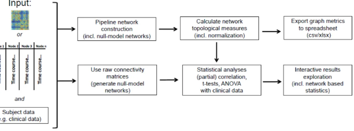
Figure 3.5: Schematic workflow of GraphVar. Adapted from (Kruschwitz et al.,2015)
3.4.1 GraphVar - overview
Since GraphVar is a very new tool and will be the basis for most of analysis performed in this thesis, it will be given a general explanation of its operation. The use of this tool involved talking with the lead author, Johann Kruschwitz from Charité - Universitätsmedi-zin Berlin, in order to fix some bugs as well as adapt the tool to undirected connectivity matrices when doing raw matrix analysis (it was just allowed to network construction and characterization analysis ). Figure 3.5 depicts the schematic workflow of GraphVar.
GraphVar accepts anynxnmatrix containing information about connectivity among network nodes in .mat format. It can also generate connectivity matrices based on Pearson correlation, partial correlation, spearman correlation, percentage bend correlation or mutual information from input time series. However this functionality is not applied in this project since the connectivity matrices were obtained using the above methodologies. Along with the connectivity matrices GraphVar requires a parcellation scheme for the brain (e.g AAL atlas) thereby defining the nodes of the network in spread sheet format (.csv or excel). There is no limit to a specific number of nodes and the user can define the brain parcellation scheme according to his or her requirements. Moreover, GraphVar provides statistical analysis functions on network pipeline and raw connectivity matrices such as correlations or group comparisons. Thus, one may enter demographic, clinic, or other subject specific data (.csv or excel) for statistical analysis.
GraphVar offers two different analysis possibilities: a pipeline construction of graph networks in order to calculate network topological measures and a direct use of raw connectivity matrices (Figure 3.6).
3.4.1.1 Raw connectivity matrix