Vision Based Obstacle Detection for All-Terrain Robots

(1)

Magno Edgar da Silva Guedes

Vision Based Obstacle Detection

for All-Terrain Robots

(2)

(3)

UNIVERSIDADE NOVA DE LISBOA

Faculdade de Ciˆencias e Tecnologia

Departamento de Engenharia Electrot´ecnica

e de Computadores

Vision Based Obstacle Detection for All-Terrain Robots

Magno Edgar da Silva Guedes

Dissertação apresentada na Faculdade de Ciências e Tecnologia da

Universidade Nova de Lisboa para obtenc¸˜ao do grau de Mestre em

Engenharia Electrot´ecnica e de Computadores.

Orientador:

Prof. Jos´e Ant´onio Barata de Oliveira

(4)

(5)

Acknowledgements

First of all, I would like to express my sincere gratitude to my dissertation supervisor, Prof.

Jos´e Barata, for the opportunity, motivation and support, and to Pedro Santana for all the

sup-port, fruitful comments and valuable help.

I would also like to thank my parents Aur´elio and Florinda and my brother Quim for giving

(6)

(7)

Eles não sabem, nem sonham, que o sonho comanda a vida, que sempre que um homem sonha o mundo pula e avança como bola colorida entre as mãos de uma criança.

(8)

(9)

Resumo

Esta dissertação apresenta uma solução para o problema da detecção de obstáculos em

am-bientes todo-o-terreno, com particular interesse para robôs móveis equipados com visão

estere-osc´opica. Apesar das vantagens da vis˜ao, sobre outros tipos de sensores, tais como o custo,

peso e consumo energético reduzidos, a sua utilização ainda apresenta uma série de desafios.

Tais desafios incluem a dificuldade em lidar com a considerável quantidade de informação

ger-ada e a robustez necess´aria para acomodar n´ıveis altos de ru´ıdo. Estes problemas podem ser

atenuados por pressupostos r´ıgidos, tal como considerar que o terreno à frente do robô é

pla-nar. Apesar de permitir um menor custo computacional, estas simplificações não são

neces-sariamente aceit´aveis em ambientes mais complexos, onde o terreno pode ser mais irregular.

Esta dissertação propõe a extensão de um conhecido detector de obstáculos que, por relaxar a

assumpção do plano é mais adequado para ambientes não estruturados. As extensões propostas

são: (1) a introdução de um mecanismo de saliência visual para focar a detecção em regiões

mais prováveis de conter obstáculos; (2) filtros de votação para diminuir a sensibilidade ao

ru´ıdo; e (3) a fus˜ao do detector com um m´etodo complementar por forma a criar um sistema

h´ıbrido e, portanto mais robusto. Resultados experimentais obtidos com imagens de ambientes

todo-o-terreno mostram que as extens˜oes propostas permitem um aumento de robustez e

(10)

(11)

Abstract

This dissertation presents a solution to the problem of obstacle detection in all-terrain

en-vironments, with particular interest for mobile robots equipped with a stereo vision sensor.

Despite the advantages of vision, over other kind of sensors, such as low cost, light weight and

reduced energetic footprint, its usage still presents a series of challenges. These include the

dif-ficulty in dealing with the considerable amount of generated data, and the robustness required

to manage high levels of noise. Such problems can be diminished by making hard assumptions,

like considering that the terrain in front of the robot is planar. Although computation can be

considerably saved, such simplifications are not necessarily acceptable in more complex

envi-ronments, where the terrain may be considerably uneven. This dissertation proposes to extend

a well known obstacle detector that relaxes the aforementioned planar terrain assumption, thus

rendering it more adequate for unstructured environments. The proposed extensions involve:

(1) the introduction of a visual saliency mechanism to focus the detection in regions most likely

to contain obstacles; (2) voting filters to diminish sensibility to noise; and (3) the fusion of

the detector with a complementary method to create a hybrid solution, and thus, more robust.

Experimental results obtained with demanding all-terrain images show that, with the proposed

extensions, an increment in terms of robustness and computational efficiency over the original

(12)

(13)

List of Symbols and Notations

Symbol Description

OD Obstacle Detector

OOD Original Obstacle Detector [Manduchi et al., 2005]

EOD Extended Obstacle Detector [Santana et al., 2008]

SalOD Saliency Based Obstacle Detector [Santana et al., 2009]

ESalOD Extended Saliency Based Obstacle Detector [Santana et al., 2010]

ROC Receiver Operating Characteristic

TPR True Positive Rate

FPR False Positive Rate

θ minimum slope a surface must have to be considered as an obstacle

Hmin minimum height an object must have to be considered an obstacle

Hmax maximum allowed height between two points to be considered

com-patible with each other

p generic 3-D data point

p′ _{projection of a generic 3-D data point}_p_{onto the image plane}

CU upper truncated cone (for compatibility test)

C′

U upper truncated triangle (result from projectingCU onto the image

plane)

CL lower truncated cone (for compatibility test) C′

(14)

Symbol Description

r range for ground plane estimation

t minimum area a triangle, defined by three 3-D points, must have in

order to the points be considered collinear

dplane maximum distance to a potential ground plane a 3-D point must have

to pertain to the same plane

nhypo number of generated plane hypoteses for ground plane estimation

g scalling factor for ground plane estimation

α scalling factor for ground plane estimation

n base resolution for space-variant resolution

m base resolution for rough analysis in space-variant resolution

nslide maximum number of consecutive pixels skipped in SalOD

nmax maximum number of consecutive pixels skipped in ESalOD

w radius of scan window for the region growing process

d maximum distance between two points to be aggregated in the region

growing process

v voting filter threshold

(15)

List of Figures

2.1 Visual processing diagram for obstacle detection in flat terrains. . . 27

2.2 Overview of the obstacle detection algorithm for curved terrains. . . 28

2.3 The three structure classes structure that 3-D data can be classified into. . . 30

2.4 Example in side-view for the cone based obstacle detection technique. . . 32

3.1 Example of a 3D point cloud. . . 36

3.2 (a) Disparity calculation. (b) Disparity map. . . 37

3.3 Saliency computation and ground-plane estimation results. . . 41

4.1 Geometric interpretation of the base model [Manduchi et al., 2005]. . . 45

4.2 Projection of the truncated conesCU onto the image plane. . . 46

4.3 Compatibility test on a real image. . . 47

4.4 Voting mechanism [Santana et al., 2008]. . . 51

4.5 Obstacle detection results. . . 54

5.1 Architecture for hybrid obstacle detection. . . 56

5.2 Hybrid Obstacle Detector results. . . 57

5.3 Graphical representation of the weighted votes. . . 59

5.4 Cost map results. . . 60

6.1 Base resolution selection. . . 62

6.2 Impact of the area filter. . . 64

(20)

6.4 Computation time comparison . . . 66

6.5 Analysis of the best configuration for the plane-based detector. . . 68

6.6 Comparison between fusion and isolated obstacle detection methods. . . 68

6.7 Correlation map between the system’s output and the ground truth. . . 69

A.1 Left-camera images encompassing the dataset used in all experiments. . . 83

A.2 Saliency maps obtained from each image in the dataset. . . 84

A.3 Obstacle-ground truth hand-drawed for each image in the dataset. . . 85

A.4 Detection results obtained from all the images in the dataset for ESalOD . . . . 86

A.5 Correlation maps between the obstacle-ground truth and the system output . . . 87

A.6 Detection results obtained from all the images in the dataset for Hibrid OD . . . 88

(21)

Chapter 1 Introduction

Over the past few years, we have been observing an increasing interest on unmanned

all-terrain vehicles [Matthies et al., 2007]. From military operations [Bellutta et al., 2000] to

in-terplanetary exploration [Maimone et al., 2006], from rescue missions [Birk and Carpin, 2006]

to wide-area surveillance and humanitarian demining [Santana et al., 2007], their presence is

increasingly noticeable. Although the man-in-the-loop is often required for the control of high

level operations, service robots must integrate autonomous capabilities, such as obstacle

detec-tion and avoidance, in order to move safely [Kim et al., 2006], [Matthies et al., 2007].

Despite the long research history in obstacle detection, a set of hard challenges are still to be

tackled if the targeted environments are unstructured. This dissertation contributes to this line

of research by proposing a reliable and computationally efficient obstacle detector for off-road

environments. Efficiency here is particularly interesting to enable consumer robotics, which

must be cheap. Therefore, expensive sensors or computational units must be avoided.

In order to perceive their surroundings, robots are normally equipped with a wide variety

of sensors [Thrun et al., 2006], including Global Positioning Systems (GPS), Inertial

Measure-ment Units (IMU), Radio Detection and Ranging Systems (RADAR), Laser Scanners (LADAR)

or Stereoscopic Cameras. However, integrating all this equipment in low cost or small robots,

where space and energy storage are limited, is quite challenging. From the aforementioned

(22)

characterisation of unknown scenarios [Lalonde et al., 2006], [Manduchi et al., 2005]. These

two types of sensors are complementary and consequently desirable. In particular, stereo

vi-sion overcomes several limitations of laser scanners, such as sensitivity to vibration due to

mechanical components, active interaction with the environment, slow 3D reconstruction, low

resolution, and absence of colour information. Moreover, vision systems aggregates a set of

important features for all-terrain service robots, such as general purpose capabilities, small

en-ergetic footprint, light weight, small size and low cost. Due to these reasons, stereo vision

has been selected in the context of this work. However, despite the mentioned advantages, the

large amount of generated data, which is also noisy, allied to the unstructured nature of off-road

environments makes the use of stereo vision for robust and fast obstacle detection a still open

problem.

A common approach to reduce its computational cost is to introduce some assumptions, such

as some form of structure. A typical one is that obstacles are 3-D points standing above a flat

ground [Konolige et al., 2006], [Broggi et al., 2006]. However, off-road terrains are often rough

and hardly flat, which makes this approach quite unsuitable. A more comprehensive technique

is the fitting of several planes to several parts of the environment, and use their residual as

a measure of traversability [Singh et al., 2000], [Goldberg et al., 2002]. One limitation of this

method is the computational cost associated to the multiple fitting processes. Another limitation

is related to its heuristic nature, which complicates the task of specifying the proper size of the

planes and what an obstacle is, taking into account a specific robot’s physical apparatus. A

more complete, yet too expensive solution, is to generate a digital elevation map, upon which

trajectories are planned according to models of interaction between the robot and the terrain

[Lacroix et al., 2002]. Another known approach is to characterise obstacles in terms of the

statistics governing patches of accurate 3-D point clouds [Lalonde et al., 2006]. However, such

accuracy is only attainable with laser scanners. A more useful technique for stereo vision and, in

particular, for outdoor environments is to define obstacles in terms of geometrical relationships

between their composing 3-D points, as proposed by Manduchi et al. [Manduchi et al., 2005].

(23)

In order to reduce both noise sensitivity and computational cost, the detector was recently

extended by Santana et al. [Santana et al., 2008]. However, the proposed extensions are too

rigid, i.e. noise and computational time are reduced at the expense of a reduction in terms of

true positive rate. Bearing what have been said, this dissertation describes the research work that

was carried out to improve robot obstacle detection. In particular, the work was concentrated

on improving the previously mentioned algorithm in order to increase accuracy, robustness and

computational efficiency.

1.1 Problem Statement

As previously stated, this dissertation intends to develop a pure vision-based obstacle

detec-tor for all-terrain service robots. In order to achieve this, three main problems must be taken

into consideration:

1. The proposed model must be suitable for off-road environments, where both structured

and unstructured surfaces must be correctly identified either as obstacles or free-space.

Obstacles here are defined as anything that can block the passage of a wheeled robot.

2. The proposed model must be robust to noisy data, typical of a stereo vision-based system.

Noise may be induced by several different factors (e.g. insufficient illumination,

exces-sive light exposure, dirty lens, uncalibrated cameras, etc.) and inevitably affects the 3-D

reconstruction process.

3. The proposed model must be computationally efficient and cope with real-time

con-straints, so that the robot can drive safely in demanding environments. As 3-D stereo

reconstruction generates dense point clouds, the analysis of such data is often expensive.

Thus, maintaining low complexity and improved efficiency can be particularly

(24)

1.2 Solution Prospect

This dissertation proposes the following solutions for the identified problems:

1. Obstacles will be defined according to the geometrical relationships between their

com-posing 3-D points, as in the model proposed by Manduchi et al. [Manduchi et al., 2005].

By adopting this model, hard assumptions about the terrain’s topology are discarded and

surfaces will be considered as obstacles if their slope or height are higher than the

max-imum a wheeled robot can climb or step over. Additionally, a hybrid architecture is

presented where the proposed model is integrated with a detector that makes the plane

as-sumption. This architecture allows the exploitation of the complementary role exhibited

by both detectors, i.e. to increase in true positive rate and to reduce in computation time.

2. Noise will be reduced by means of a robust filtering mechanism. This mechanism

consists on a remodelled version of the voting filters introduced by Santana et al. [Santana et al., 2008]. Briefly, each time a pair of related 3-D data points are

consid-ered to pertain to an obstacle, each one of them cast avote. By the end of the analysis, the morevotesa potential obstacle point have, less likely is to be an outlier erroneously computed from 3-D reconstruction. This dissertation adds scale invariance to the voting

mechanism. Additionally, potential obstacles are segmented and the number of points

each segment contains is thresholded by a novelarea filter, eliminating sparse noisy data.

3. Computational efficiency will be improved by a saliency-based space-variant resolution

mechanism. The space-variant resolution mechanism was also proposed by Santana et

al. [Santana et al., 2008] in order to reduce the number of pixels being analysed, thus

saving computation time. This dissertation uses visual saliency in order to modulate the

space-variant resolution, so that the most important regions, i.e. regions that are prone to

contain obstacles, are analysed with more detail. This not only improves efficiency, but

(25)

1.3 Dissertation Outline

This dissertation is organised as follows:

Chapter 2gives a brief overview of the state of the art regarding obstacle detection techniques

for off-road environments;

Chapter 3describes the supporting mechanisms for the developed algorithm, such as the

dis-parity calculation, saliency computation and ground plane estimation.

Chapter 4describes a full obstacle detector suited for autonomous mobile robots equipped with

a stereo vision sensor and operating in rough and unstructured outdoor environments;

Chapter 5 presents an improved obstacle detection architecture that integrates two different

techniques in an efficient way;

Chapter 6presents a set of experimental results, which encompasses a comparative analysis

between the developed model and its predecessors.

(26)

1.4

Chapter 2 State of the Art

This chapter surveys the state of the art in off-road obstacle detection algorithms. In the

past10years, there has been extensive research on obstacle detection techniques for all-terrain

service robots, mainly due to the challenging problem of properly distinguish obstacles in rough

and unstructured natural environments. This problem have promoted several approaches in the

search for better solutions.

Hence, herein is presented an overview of the most successful approaches to solve the

prob-lem previously mentioned.

The flat terrain assumption or flat world approach (section 2.1) is a well known method that

takes advantage of simplifications in order to reduce complexity and accelerate the detection

process. However, as the name suggests, work well when the terrain is relatively plane but fails

in rough areas. Next, a similar approach is taken so as to improve detection in curved terrains

by assuming that the plane show smooth slope variations (section 2.2), which is not necessarily

the case in off-road. A more comprehensive approach is to characterise obstacles by means of

a traversability cost (section 2.3). However, this technique requires the construction of local

maps containing the terrain’s topology, which is computationally expensive and needs high

storage capability. Loosing the necessity for topology understanding of the terrain, obstacles

can be characterised directly from a statistical analysis of its composing 3-D points (section 2.4).

(28)

laser scanners, thus is more applicable with data obtained by a laser scanner than the more

noisy data obtained by stereo vision. Finally, a more useful technique for vision systems is to

define obstacles in terms of geometric relationships between 3-D data points (section 2.5). This

method is more robust, still the involved complexity requires a comprehensive solution in order

to reduce computational cost.

The expensive computation of the referred techniques lies mainly in the large amount of

data that have to be analysed. This fact can be circumvented if the region of analysis is reduced.

However, the problem is to know which regions should be analysed. An efficient method

capa-ble of selecting interest regions is the application of visual attention mechanisms. Section 2.6

survey some of the attention mechanisms that are prone to be applied in mobile robotics.

2.1 Flat Terrain Assumption

Although off-road environments are quite marked by their irregularity, it is often possible to

determine a dominant ground plane in the robot’s surroundings. The presence of a ground plane

is of major importance for reducing the complexity of the assumptions needed to be made in

order to characterise obstacles. Moreover, assuming that the robot is navigating in a relatively

flat terrain, obstacles can be simply characterised as prominent surfaces standing above the

ground.

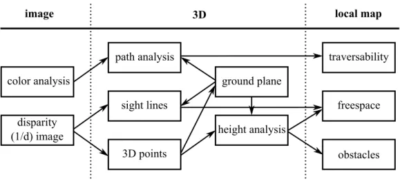
In the model proposed by Konolige et al. [Konolige et al., 2006], the robot is assumed to

navigate on a locally flat ground. In this case, obstacles near to the robot’s location can be

detected by thresholding the height of 3-D points standing above the ground plane. Fig. 2.1

depicts the proposed model to detect and map obstacles in the robot’s surroundings. First,

dis-parity and colour images are obtained from a stereo camera. Then, the 3-D point cloud is

com-puted from the disparity image and the ground plane is extracted using a RANSAC technique

[Fischler and Bolles, 1981]. 3-D points that lie too high above the ground plane, but lower than

the robot’s height, are labelled as obstacles and sight lines, i.e. columns of ground plane pixels

(29)

image disparity (1/d) image color analysis 3D points path analysis sight lines height analysis ground plane obstacles traversability freespace

3D local map

Figure 2.1: Visual processing diagram for obstacle detection in flat terrains as proposed by Konolige et al. [Konolige et al., 2006].

colour image is used by the algorithm to learn traversable paths.

Alternatively, Broggi et al. [Broggi et al., 2006] proposes to detect obstacles directly in

the disparity images, rather than performing a 3-D reconstruction of the environment. Hence,

detection is made by applying several filters to the disparity image in order to confine disparity

concentrations that are eligible to be obstacles. With this, computational time is saved but the

model are limited to specific types of obstacles. In fact, in this particular case, the model can

only successfully detect thin tall obstacles or large obstacles’ edges while untextured obstacles

are detected with a laser scanner.

Although these approaches work well for flat terrains, they fail in rougher ones, which is

typically the case in off-road.

2.2 OD in Terrains with Smooth Slope Variations

In the previous section, a flat terrain was assumed. However, apart from taking into account

the presence or not of a dominant ground plane, natural terrains are hardly flat. An approach that

deals with non-flat terrains is proposed by Batavia and Singh [Batavia and Singh, 2002]. Their

model is suited for cases where the terrain has significant curvature but is smooth enough to

(30)

single-scan profile cartesian view

NN fusing filtered results

Figure 2.2: Overview of the obstacle detection algorithm for curved terrains as proposed in [Batavia and Singh, 2002].

model is similar to the one presented earlier, i.e. to find prominent surfaces above the ground,

the difference lies in the ground’s topology. In their work, Batavia and Singh use a 2-axis laser

scanner as the input sensor. The obstacle detection algorithm is depicted in Fig. 2.2 and consists

of two stages: classification and clustering (fusion). In the classification stage, each range point

scanned is classified asobstacle or freespaceif it represents or not a discontinuity across the ground curve. The ground curvature is estimated by converting the laser data into Cartesian

coordinates and calculate the resulting gradient. Scans are then accumulated in a time window

in order to determine the amount of data that will be fused in the next stage. In the fusion stage,

pixels classified as obstacles are clustered using a nearest-neighbour (NN) criterion, and then

candidate obstacles are filtered based on their mass and size.

Being more generic than the previous assumption, this approach still doesn’t fit well with

the reality of off-road environments.

2.3 Traversability and Elevation Maps

Rather that assuming a typical geometry for the terrain (flat or curved), a more

comprehen-sive solution have also been studied, which consist on fitting several planes to different parts of

(31)

by Goldberg et al. [Goldberg et al., 2002] and Hamner et al. [Hamner et al., 2008]. Differently

from deciding if a certain region in the environment corresponds to an obstacle that the robot

should avoid or a free space where the robot may navigate freely, traversability offers the

pos-sibility for the robot to negotiate a trajectory over that region trading off between the potential

cost of passing through versus opt for a longer route.

The concept consists on creating grid-based local traversability maps, where obstacles are

represented in terms of the level of hazardness associated to each cell. Briefly, the system starts

by collecting, for each cell, the first and second moment statistics about all the range points

(acquired from the input sensor and expressed in the coordinate frame of the local map) that

falls inside that cell. Then, for each cell, the moment statistics from a robot-sized patch of

surrounding cells are merged in order to find the best-fit plane. The resulting plane parameters

are used to compute an hazard level that corresponds to the traversability cost of the cell.

Following the idea of traversability measures, a similar procedure is also presented in Lacaze

et al. [Lacaze et al., 2002]. In the later, vehicle masks are placed along potential trajectories in

an elevation map in order to predict pitch and roll along the paths. Thus, plane fitting is only

done along the estimated paths. The pitch and roll measures are used to estimate the cost of

traversing each path.

One limitation of these methods, however, is the computational cost associated to the

mul-tiple fitting processes and storage requirements. Another limitation concerns with its heuristic

nature, which complicates the task of specifying the proper size of the planes and what an

obstacle is, taking into account a specific robot’s physical apparatus.

Lacroix et al. [Lacroix et al., 2002] proposes a model to predict the chassis attitude and the

internal configurations of the robot for several positions along a trajectory arc over a digitalised

elevation map. Prediction is made by a geometric placement function that modulate the

inter-action between the robot and the terrain. The predicted configurations are used to compute the

(32)

λ

0

λ

1

Figure 2.3: The three types of structure that 3-D data can be classified into (left: scattered regions, middle: linear structures, right: planar surfaces) [Lalonde et al., 2006].

2.4 Statistic Analysis of 3-D Data

All previous approaches focused on finding prominent surfaces on the ground or estimate

trajectories based on the ground’s features. However, such approaches are best applied in

smooth terrains. For rougher or vegetated terrain, a different analysis criteria is needed.

A well known solution for this aspect interpret the statistics governing 3-D point clouds in

order to classify visible surfaces in the environment. This solution, proposed by Vandapel et

al. [Vandapel et al., 2004] and later by Lalonde et al. [Lalonde et al., 2006] uses the spatial

distribution of the generated 3-D point cloud to classify regions into surfaces, linear structures

and vegetation. The classification is done by first computing the eigenvalues of the covariance

matrix for all the points within a neighbourhood of the point of interest and inspect the relative

magnitudes of those eigenvalues. The vegetation, typically scattered points have no dominant

eigenvalue, linear structures have one dominant eigenvalue and solid surfaces have two

dom-inant eigenvalues (see Fig. 2.3). Also, the estimated ground plane of the local area can be

recovered by this method as it is the eigenvector corresponding to the smallest eigenvalue of the

covariance matrix.

However, this method requires accurate 3-D point registration, thus is more applicable with

(33)

2.5 Geometrical Relationships in 3-D Point Clouds

An approach that have been attracting particular interest, mainly due to its correctness is the

one that define obstacles in terms of geometrical relationships between their composing 3-D

points. By inspecting such relationships it is possible to efficiently consider visible surfaces

whose geometric properties represent a real obstacle to the robot, because they are too high or

too inclined for the robot to pass through.

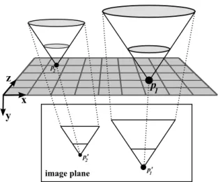
In the work of Manduchi et al. [Manduchi et al., 2005], an outstanding definition of obstacle

is presented by introducing the concept of compatibility between pairs of 3-D points.

Briefly, a visible surface is considered part of an obstacle if its slope is larger than a certain

valueθ, representing the higher slope a robot can climb, and if it spans a vertical interval larger

than a threshold H, representing the height an obstacle must have to block the robot from

passing through. In order to apply this concept to arbitrarily shaped surfaces, slope and height

measures are taken from pairs of 3-D points and those who have the conditions to pertain to

the same surface and to be considered as obstacles are denoted compatibles. A more extensive

explanation about compatibility will be given in section 4.1.

By this model, any surface point is considered an obstacle if there is at least one other point

pertaining the same surface whose distance is within a certain interval and the line connecting

them presents a slope higher thanθ. The geometrical interpretation that can be made from this is

that spanning an inverted truncated cone, with its vertex in a surface point and aligned upwards

or downwards, if it encompasses another surface point, then both the vertex point and all the

points encompassed by the cones are considered compatible and therefore, obstacle points (see

Fig. 2.4).

In spite of its applicability for detecting obstacles in rough terrains, this approach suffers

from a high sensitivity to noisy data and a excessive computational cost.

Several improvements over the original approach have been made in order to attenuate those

issues. In [van der Mark et al., 2007] computation time was reduced by extensive use of lookup

(34)

Figure 2.4: Example in side-view for the process of classifying obstacle points (filled dots) by the method proposed in [Manduchi et al., 2005]. For the sake of readability, only the upper truncated cones are represented.

possible to better detect far obstacles besides the problem that accuracy in 3-D reconstruction

decreases with distance and hence, obstacle points appear more sparse. However, trying to

detect far obstacles in a bad signal-to-noise ratio is not mandatory. Instead, reliable detection

of obstacles with a low false positive rate, in the robot surroundings, its a more important issue

that still have to be solved

In the work of Santana et. al [Santana et al., 2008], efforts where made in order to reduce

computational cost of the original method by fastening the process of checking for compatible

points, applying a space-variant resolution mechanism that will be described in section 4.2.

Also, Santana et al. introduced two voting filters embedded in the original obstacle detection

algorithm so as to reduce its sensitivity to noise. These voting filters will be also described in

section 4.3.

In the later, the voting filters are too strong, influencing negatively the true positive rate.

Also, they are not scalable, which means that far obstacles, represented by fewer 3-D points are

more prone to be eliminated than closer ones. On the other hand, the space-variant resolution

operates to great extent blindly, i.e. in order to reduce computational cost, many pixels are

skipped. However, it would be useful to known whose pixels should be skipped and whose

should be analysed. This selection process can be carried out by a visual attention mechanism

(35)

2.6 Visual Attention Mechanisms

Recent research in the field of mobile robotics have shown the applicability of visual

atten-tion mechanisms in order to guide expensive tasks such as object detecatten-tion and characterisaatten-tion,

reducing the region of interest and, consequently, saving computation time.

Hong et al. [Hong et al., 2002] uses prediction to focus a colour-based detector of puddles

and road signs. Prediction, in this case, is no more than collecting laser and colour camera

data into a world model and, given the actual position of the robot in the world model and the

information previously obtained, estimate which regions of future images shall be analysed.

In a more active way, visual saliency has been used to control the gaze of a humanoid

head (e.g. [Vijayakumar et al., 2001], [Orabona et al., 2005], [Mor´en et al., 2008]), or to detect

objects in domestic environments (e.g. [Meger et al., 2008], [Yu et al., 2007]).

Besides object detection, visual saliency has also been used to select strong landmarks

for visual self-localisation and mapping in urban environments (e.g. [Newman and Ho, 2005],

[Frintrop et al., 2007]).

Except for the first case, all the previous applications are restricted to indoor or urban

en-vironments. In the unstructured off-road environments, obstacles are not necessarily the most

(36)

(37)

Chapter 3 Supporting Mechanisms

This chapter summarises the mechanisms that will serve as support for the obstacle detection

algorithm, namely the calculation of stereo disparity, the computation of saliency maps and

the estimation of the dominant ground plane. Stereo disparity allows the computation of 3-D

point clouds, i.e. a three-dimensional representation of the scene captured by the stereo sensor.

Saliency maps will be used to guide the detector through regions where obstacles detach more

significantly from the background. Finally, ground plane estimation determines the orientation

of the dominant ground plane next to the robot location.

3.1 Stereo Vision

The model proposed in this dissertation uses dense 3D point clouds (see Fig. 3.1) in order

to detect obstacles. Thus, an efficient method for calculating such point clouds is required. The

use of stereo vision was adopted for this purpose.

Briefly, a pair of cameras internally and externally calibrated, and displaced horizontally

from one another, gives a right and left image. Both images are then used to find matching

elements, i.e. elements in the right image that have high similarities with elements in the left

image. Calculating the disparity of the matched elements enables the estimation of their

(38)

Figure 3.1: Example of a 3D point cloud obtained using the Small Vision System framework [Konolige and Beymer, 2007].

3.1.1 Disparity

Disparity is defined by the difference in image location of an object. In stereo vision,

dis-parity is used to estimate the range of objects captured by the stereo sensor. The distance from

the camera to a given object is calculated by triangulation. Fig 3.2(a) exemplifies the process

assuming that both images are embedded within the same plane. This can be achieved by

pre-cise camera alignment. In order to calculate disparity, it’s needed to find the objects location

in both images. With this setup, disparity is only observed horizontally, i.e. a point projected

within a given row of the left image must project in the same row of the right image, which

reduce the search space. Fig 3.2(b) depicts a typical disparity map where pixel intensities are

related to computed range.

3.2 Saliency Computation

The following describes the biologically inspired saliency model. It is a specialisation for

off-road environments of the one proposed by Itti et al. [Itti et al., 1998]. LetLbe the left image,

with widthwand heighth, provided by the stereo vision sensor. To reduce computational cost,

saliency is computed on a region of interest (ROI) ofL. TheROIis an horizontal strip between

(39)

dl dr b

f f

r

(a) (b)

Figure 3.2: (a) Disparity calculation for an object located at a distancerfrom a stereo camera with a baselineb and a focal length f. In the left image, the object is projected at a distance

dl from the centre of the image and in the right image is projected at a distance dr from the centre. Knowing the disparity valued = dl−dr, the ranger is given by r = (b·f)/d. (b) Disparity map computed with the SVS libraries [Konolige and Beymer, 2007] for the image

#24(see Fig: A.1). The gradient represents the range from nearer points (light gray) to farther ones (black). White pixels represent points with no computed range.

an associated depth within the range of interestr. To further reduce computational cost, all

image operators are performed over 8-bit images, whose magnitude is clamped to [0,255] by

thresholding.

A dyadic Gaussian pyramidI(σ)with six levelsσ ∈ {0, . . . ,5} is created from the

inten-sity channel ofROI. The resolution scale of level σ is1/2σ _{times the} _ROI _{resolution scale.}

Intensity is obtained by averaging the three colour channels. Then, four on-off centre-surround

intensity feature mapsIon−of f₍_{c, s}₎_{are created, to promote bright objects on dark backgrounds,}

in addition to four off-on centre-surround intensity feature mapsIof f−on₍_{c, s}₎_{, to promote dark}

objects on bright backgrounds.

On-off centre-surround is performed by across-scale point-by-point subtraction, between

a level c with finer scale and a level s with coarser scale (linearly interpolated to the finer

resolution), with (c, s) ∈ Ω = {(2,4),(2,5),(3,4),(3,5)}. Off-on maps are computed the

other way around, i.e. subtracting the coarse level from the finer one.

These maps are then combined to produce the intensity conspicuity map,

CI = ∑

i∈{on−of f,of f−on} (

1 2

⊕

(c,s)∈ΩI

(40)

where the across-scale addition ⊕

is performed with point-by-point addition of the maps,

properly scaled to the resolution of level σ = 3. Sixteen orientation feature maps, O(σ, θ),

are created by convolving levels σ ∈ {1, . . . ,4} with Gabor filters tuned to orientationsθ ∈

{0◦_,₄₅◦_,₉₀◦_,₁₃₅◦_}_{. Gabor filters are themselves centsurround operators and therefore}

re-quire no across-scale subtraction procedure [Frintrop, 2006]. As before, all orientation feature

maps are combined at the resolution of levelσ= 3in order to create the orientations conspicuity

map,

CO =∑_θ_∈{₀◦_,45◦_,90◦_,135◦_}

( 1 4

⊕

σ∈{1,...,4}O(σ, θ) )

.

The saliency map S is obtained by modulating the intensity conspicuity mapCI with the

orientations one CO, S = M(1₂ · N(CI),₂1 · N(CO)), where M(A, B) = A·sigm(B),

be-ing sigm(.) the sigmoid operator andN(.) rescales the provided image’s amplitude between

[0,255]. Fig. 3.3(a) depicts a saliency map generated by this method.

The proposed saliency model is essentially based on the model proposed by [Itti et al., 1998]

but considering both on-off and off-on feature channels separately, which has been shown to

yield better results [Frintrop, 2006]. Still, two major innovations are present in the proposed

model. First, the normalisation operatorN(.)does not try to promote maps according to their

number of activity peaks, as typically done. The promotion of some maps over others according

to activity peaks showed to provide poor results in the tasks herein considered. This is because

spatially frequent objects, which are inhibited in typical saliency applications, may be obstacles

for the robot, and thus must also be attended.

A narrow trail may be conspicuous in the intensity channel if it is, for instance, surrounded

by dense and tall vegetation. This contradicts the goal of making obstacles salient, rather than

the background, which is why saliency is computed from the weighted product of the

conspicu-ity maps [Hwang et al., 2009] rather than their addition [Itti et al., 1998], [Frintrop, 2006]. It

focus the saliency on regions where orientations are strong, i.e. small objects, borders of

(41)

3.3 Ground Plane Estimation

The used solution to modulate the hypothesis-generation step of a conventional RANSAC

[Fischler and Bolles, 1981] robust estimation procedure is composed of the following seven

steps.

1. pick randomly a setRof three non-collinear 3-D points within ranger, and generate its

corresponding ground plane hypothesis,hR, with some straightforward geometry. Points

are considered non-collinear if the area of the triangle defined by them is above a threshold

t.

2. the score of the plane hypothesis is the cardinality of the set of its inliers, score(hR) = |PhR|. An inlier,j ∈PhR, is a 3-D point whose distance to planehR,d(j, hR), is smaller

than a given thresholddplane.

3. repeat steps 1 and 2 untilnhypohypotheses, composing a setH, have been generated.

4. select for refinement, fromH, the hypothesis with the highest score:

b = arg maxh∈Hscore(h).

5. computeb′_{, which is a refined version of}_b_{, by fitting the inliers set of the latter,}_P b. This

fitting is done with weighted least-squares orthogonal regression, via the well known

Singular Valued Decomposition (SVD) technique. The weight wq of an inlier q ∈ Pb is

given bywq = 1− _dd(q,b)

plane. That is, the fartherqis fromb, the less it weights in the fitting

process. Compute the inliers set of b′_, _P

b′, and substitute the current best ground plane estimate by the refined one, i.e. makeb =b′_and_P

b =Pb′.

6. iterate step 5 until|Pb|becomes constant across iterations or a maximum number of

iter-ations,mref it, is reached.

(42)

To take saliency into account, each 3-D pointpselected to build an hypothesis in step 1 must

pass a second verification step. This step reduces the chances of selectingpproportionally to

thelocal saliencyof its projected pixelp′_{. The underlying empirical assumption is that saliency}

is positively correlated with the presence of obstacles. Preferring non-salient points thus raises

the chances of selecting ground pixels (see Fig 3.3(e)).

Formally, a 3-D point p is rejected in the second verification step if sp′ > P_α(x)

·nl, where:

nl ∈ [0,1]is the number of pixels with saliency below a given threshold l normalised by the

total number of pixels; local saliency sp′ ∈ [0,255] is the maximum saliency within a given sub-sampled chess-like squared neighbourhood of p′_{, with size} _g_·_n

l, being g the empirically

defined maximum size; P(x) ∈ [0,255] represents samples from an uniform distribution; and

α is an empirically defined scaling factor. The goal of using the normalised number of pixels

with a saliency value under a given threshold is to allow the system to progressively fall-back

to a non-modulated procedure as saliency reduces its discriminative power, i.e. it is too spread

in space. This happens for instance in too textured terrains, in which the sampling procedure is

(43)

(a)

(b) (c)

(d) (e)

(44)

(45)

Chapter 4 Obstacle Detection Core

This chapter presents a full obstacle detector suited for autonomous mobile robots operating

in rough and unstructured outdoor environments, and equipped with a stereo vision sensor.

Since, in such environments, little assumptions can be made about the morphology of a typical

obstacle, Manduchi et al. [Manduchi et al., 2005] proposed a method for defining local obstacle

points based on the relationship between pairs of 3-D data points. Such definition, described

in section 4.1 serves as a basis for the work presented in this dissertation in which a

space-variant resolution mechanism modulated by saliency, described in section 4.2, and a voting

filter, described in section 4.3 are used in order to reduce both computation time and noise

sensitivity. Section 4.4 describes a method to isolate the detected objects and discard the ones

that are small enough not to be considered as obstacles.

4.1 Obstacle Definition

As previously mentioned, cross-country environments usually don’t have large planar

sur-faces where obstacles just pop out from the ground. In this case, having a model that classify

obstacles based on their heights according to the global ground plane is unreliable, thus a more

comprehensive approach is needed. In literature a suitable definition of obstacle in typical

(46)

denominated Original Obstacle Detector (OOD), obstacles are defined as follows:

Definition 1: Two 3-D pointspa = (xa, ya, za)andpb = (xb, yb, zb)are considered compatible

with each other if the following conditions are both met:

1. Hmin <|yb−ya|< Hmax

2. |yb−ya|

kpb−pak

>sinθ

where,θis the minimum slope a surface must have to be considered as an obstacle,Hminis the

minimum height an object must have to be considered an obstacle, andHmax is the maximum

allowed height between two points to be considered compatible with each other.

Definition 2:Two 3-D pointspa= (xa, ya, za)andpb = (xb, yb, zb)pertain to the same obstacle

if at least one of the following conditions is met:

1. paandpb are compatible with each other;

2. paandpb are linked by a chain of compatible point pairs.

For a better understanding of how an obstacle can be specified by these conditions, the

compatibility relationship expressed inDefinition 1may be interpreted geometrically as follows: considering a 3-D point p, its compatible points are those who are spatially positioned inside

two truncated cones CU and CL with vertex in p, both oriented vertically (i.e. along the

y-axis) and symmetrical between each other, with an aperture angle of(π−2θ)and limited by

y=Hmin andy=Hmax(see Fig. 4.1).

Note that θ and Hmin are closely related with the robot’s technical and physical

specifi-cations. In fact, θ can be described as the maximum inclination a surface must have to be

climbable by the robot, whileHmin is actually the height of the free space between the ground

and the robot where small objects may be stepped over without harming the robot’s structure.

(47)

Figure 4.1: Geometric interpretation of the base model [Manduchi et al., 2005] where filled and unfilled circles represent points that are compatible and incompatible, respectively, withp. For readability reasons,CLis not represented in the figure.

point cloud result on the obstacle points being located far apart from each other which, for a

lowHmax may result in over-segmentation or even having obstacle points not to be considered

as such. However, a Hmax excessively high have the consequence of increasing substantially

the number of points to be analysed and, consequently, increase the computation time of the

OD algorithm, as will be seen in the next section.

4.2 OD Algorithm

The previous section described the way two 3-D data points must be related in order to be

considered as obstacle points.

In this section, we will see how the process of checking the set of 3-D points, given by the

stereo sensor, is made. The 3-D point cloud is computed as in [Konolige and Beymer, 2007].

As previously seen, the task of finding obstacles in a 3-D point cloud implies looking at

pairs of compatible pixels. Rather than looking to all the possible pairs of points from the point

cloud, which would result in a number ofN2₋_N _{tests, with}_N _{the total number of computed}

3-D points, Manduchi et al. [Manduchi et al., 2005] demonstrated that, actually, only a reduced

subset of pixels is needed. That is, beingp′ _{the projection of the 3-D point}_p _{onto the image}

(48)

p 1 p 2 p'₂ p'₁ image plane

Figure 4.2: Projection of the truncated conesCUonto the image plane, resulting in the truncated

trianglesC′ U.

project onto two truncated triangles C′

U and CL′ in the same image plane and with vertex in p′ (see Fig. 4.2). Also, has been demonstrated that, by scanning the pixels in the range image starting from bottom to it’s top and from left to right, it suffices to consider only the upper

truncated triangle C′

U to efficiently detect obstacle points. Bearing this in mind, the task of

checking for the compatibility points of pmeans applying the compatibility test to the points

projected inside theC′

U relative to p′. If compatible points are found, all of them as well asp′

are labelled as obstacle points.

When projecting the truncated cone onto the image plane, the correspondent truncated

tri-angle’s height is given by Hmaxf

pz

, wherefis the camera’s focal length, and base approximately

equal to 2Hmaxf

tanθmaxpzcosv

, withv = arctanpx

pz

.

4.2.1 Tilt-Roll Compensation

All the above geometrical considerations assume that the camera is not tilted nor rolled in

respect to the ground-plane. This is an obviously unbearable constraint for all-terrain robots. In

the original approach [Manduchi et al., 2005], the authors compensate small variations on the

camera’s attitude by overestimating the truncated triangle size. This approximation inevitably

increases the computational cost, and thus should be discarded.

(49)

Figure 4.3: Compatibility test on a real image. The zoomed image depicts the results of the compatibility test regarding the pixel in the truncated cone’s vertex. Red, green and black pixels overlay on the zoomed image correspond to the compatible, incompatible and without computed range points, respectively. Incompatible points show up in the truncated triangle due to perceptive. Note the rotation of the truncated triangle, which is a result of the compensation for the camera’s roll angle, with respect to the ground-plane.

magnitude. First, the dominant plane, assumed to be the ground one, is computed according to

the method proposed in section 3.3. Then, the 3-D point cloud is rotated in order to align the

world’s reference frame, given by the normal to the computed ground-plane, with the camera’s

reference frame. The projected truncated triangle is also rotated accordingly, by projecting to

the image plane the normal vector to the estimated ground plane so as the truncated triangle

be oriented along the same normal vector (see Fig. 4.3. This way, the pixels scanned in the

image plane correspond to the 3-D points that are actually encompassed by the correspondent

truncated cone.

4.2.2 Space-Variant Resolution

Despite the advantages of using a truncated triangle in order to greatly reduce the

compati-bility tests, the computational cost of the method remains too expensive. Space-variant

resolu-tion is thus essential to further reduce the computaresolu-tional load. A successful model implementing

it, from now on denominated of Extended Obstacle Detector (EOD) [Santana et al., 2008], can

(50)

For a given pixelp′_{(sequentially sampled from}₁_/n_{of the full resolution, from the image’s}

bottom to its top and from left to right), itsC′

U is first scanned for compatible points with1/m

of the maximum resolution in a chess-like pattern, wherem > n. If a compatible point with

p′ _{is found,} _C′

U is rescanned as usual with1/n of the maximum resolution (see Fig. 4.5(c) for

a graphical interpretation of this method). Then, finished the scanning procedure, the full

res-olution is recovered with the following region growing method. For each obstacle pixelp′_{, all}

its neighbours within a distancewin the image plane are also labelled obstacles if their

corre-sponding 3-D points are closer thandfromp.

Despite its considerably achievements in reducing computational cost [Santana et al., 2008],

the EOD method operates to great extent blindly. That is, in order to reduce computational cost

nandmare increased and consequently the number of skipped pixels as well. Visual saliency

(section 3.2) is known to be an important asset in many search tasks and thus it is a powerful

candidate to guide the space-variant resolution mechanism in an informed way. Bearing this in

mind, a Saliency based Obstacle Detector (SalOD) [Santana et al., 2009] is herein proposed.

Rather than applying the compatibility test along the whole scan, as performed by the OOD

[Manduchi et al., 2005], a pixelp′_{, sampled from}₁_/n_{of the full resolution is tested iff:}

1. nslideconsecutive pixels in the same row ofp′ have not been tested so far; or

2. nconsecutive pixels, after a pixel that has been tested and labelled as obstacle in the same

row ofp′_{, have not been tested so far; or}

3. there is a 10% increment between the local saliency of p′ _{and the one of its preceding}

scanned pixel, provided that both share the same row; or

4. the last scanned pixel had no computed 3-D, and hence no information could be obtained

from it.

(51)

the effects of poor light conditions, which in some situations make the top of large obstacles to

appear more salient than their bottom. If only the saliency ofp′ _{were used instead, many object}

bottom pixels would be inappropriately skipped.

Roughly speaking, the described process slides along rows for nslide pixels unless an

in-crease in saliency is observed, or something has been detected. While sliding, the compatibility

test is not performed, and consequently computational cost is saved and the chances of

gener-ating false positives is reduced. However, some additional features can be added in order to

enhance the both system’s performance and accuracy. An extended version for the SalOD is

also proposed and coined as Extended Saliency based Obstacle Detector (ESalOD).

First, in the extended version of the algorithm,p′ _{is sampled from the full resolution input}

image, so any pixel in a scanning row as a non-null probability of being assessed and, therefore

be considered as obstacle, which improve the reliability of the method.

Secondly, rather than having a fixednslide, a dynamical one is used instead,

nslide=       

k·n k < nmax

n nmax otherwise

where k is the number of consecutive times a pixel was tested and labelled as non-obstacle,

since the last time a pixel was considered an obstacle, andnmaxis an empirically defined scalar.

The application of this method results in skipping progressively more pixels as obstacles are

not found. Since the sliding process start with small jumps, the chances of failing to detect the

borders of objects are reduced.

Additionally, every time a pixelp′ _{is labelled as obstacle, the saliency of all pixels in}_C U,

i.e. within its truncated triangle, are increased in10%(empirically defined). This mechanism is

used to reinforce the presence of an obstacle by increasing the chances of a subsequent analysis

of all pixels associated with it. This is an atypical interaction between the task-specific detector

and the saliency map, as it allows the detection results to modulate the saliency map, which is

in turn guiding the detector. Typically (e.g. [Itti et al., 1998], [Frintrop, 2006]), the influence is

(52)

Also, instead of analysing every rows that are multiple ofn, as in the first approach (SalOD),

the extended (ESalOD) instead skipsn+krows, wherekis incremented every time an analysed

row does not contain any obstacle pixel. Whenever an obstacle pixel is foundk is zeroed. This

procedure, which mimics to some extent the columns sliding process, is extremely useful in

the reduction of the computation load in environments with few obstacles, or when obstacles

are mostly in the far-field. Since the truncated triangle for points in the near-field is quite large,

skipping image bottom rows when no obstacle is found there, greatly reduces the computational

cost.

A graphical representation of the space-variant resolution herein proposed is depicted in

Fig. 4.5(d).

4.3 Voting Filter

In addition to performance, both accuracy and robustness are likewise important. These two

additional ingredients, in the form of voting filters, are integral part of EOD. These filters intend

to diminish the effects caused by artifacts introduced during the 3-D reconstruction process.

In this formulation, a given point p is said to cast a number of votes equal to the number of compatible points with p, and is also said to bevoted by those points whose upper truncated cone CU include p (see Fig. 4.4). Only points that cast more than minvotes votes and are

voted more than minvoted times, simultaneously, are considered obstacles. Thus, rather than

the one-to-one mapping considered in the OOD, where compatibility is sufficient to define an

obstacle, in EOD a many-to-many mapping is necessary. This naturally results in higher levels

of robustness.

A careful observation reveals that the and operation (see above) is too strong, and con-sequently influences negatively the true positive rate. Empirical observations led to use the

conjunction operator instead, as it has been shown to foster parametrisation flexibility. This

slight change allows reducing the false positives rate by pushing further the voting thresholds,

(53)

p 1 p 3 p 2

Figure 4.4: Voting mechanism [Santana et al., 2008]. Considering that, for the sake of this example, onlyp1 andp2 were tested for compatibility,p1 is said to cast10votes whereasp3 is

said to be voted 2 times.

A mechanism to normalise the number of votes associated to each point, according to the

theoretically maximum number of possible votes, is also missing in EOD. The relevance of this issue stems from the fact that farther obstacles are represented by fewer pixels than closer

obstacles. In the algorithm herein proposed, the amount ofvotes and voted is normalised as

follows.

• Letpbe a 3-D point andp′ _{its projection in the input image.}

• LetA′

p be the set of pixels, with computed range, falling inside the truncated triangle of p′_.

• LetRp be the set of points being voted byp.

• Let B′

p be the set of pixels, with computed range, whose truncated triangles encompass p′_.

• LetSpbe the set of points voting inp.

Now, rather than comparingminvotes and minvoted againstRp andSp, respectively, as for

the OOD case, the comparison in is performed against the normalised scalars, |Rp|

|A′ p|

and |Sp|

|B′ p|

,

respectively. For the current implementation, thevotes threshold is aggregated in a single pa-rameter,v :v < |Rp|

|A′ p|

∨v < |Sp|

|B′ p|

(54)

4.4 Obstacle Segmentation

Although the focus of this work is centred in the correct and quick detection of obstacles,

an useful extra can be embedded in the algorithm in order to identify distinct obstacles in the

image. As being said in section 4.1, two 3-D pointspa and pb pertain to the same obstacle if

they are compatible with each other or linked by a chain of compatible point pairs (Definition 2). Bering this in mind, we may segment obstacles by applying an Union-Find algorithm to the points graph where compatible points are linked with each other [Manduchi et al., 2005]. Briefly, the algorithm can be explain as follows:

1. Firstly, label all points asnon-obstacles;

2. When checking the upper truncated triangle, C′

u, of a point p′, determine the set Sp′ of

compatible points withp′_.

3. IfS′

p is not empty, addp′to the set and find the point withinSp′ with the smallest label. If

all points are labelled asnon-obstacles, assign a new label to all points in S′

p, otherwise,

assign the smallest label found to all points inS′

p, keeping track of label exchanges in an

equivalence table;

4. After all points are checked, make a second pass relabelling all points with their smallest

equivalent label.

Applying this connected component labelling to the 3-D point cloud instead of applying

it onto the image plane have the advantage of properly distinguish spatially linked obstacles

even if their projections presents unconnected regions. On the other and, connected regions in

the image plane may correspond to more than one obstacle which is also considered by this

(55)

4.4.1 Area Filter

Once all obstacles are isolated, we may apply a simple rule in order to eliminate those whose

number of pixels are low enough not to be considered as obstacles. In [Manduchi et al., 2005] a

shape-based validationis proposed to achieve this goal, taking into account some 3-D attributes of the obstacles, as the volume of the 3-D bounding box around an obstacle, the average and

maximum slope of an obstacle and also its height. However, determining such attributes

cor-respond to an unnecessary addition of computation. Instead of considering such attributes, an

obstacle pointpis considered non-obstacle ifLp <100× a p2

z

, whereLp is the total number of

points with the same label aspanda is an empirically defined scalar. Although this approach

may not be very realistic in the point of view of obstacles’ morphologies, due to perspective,

experimental results prove its usefulness when in conjunction with the Voting Filter (section 4.3). In fact, theVoting Filter by itself remove most of the noise but if excessively exploited, may weaken real obstacles. In order to achieve an acceptable trade-off, some punctual noise

may remain detected as obstacle. Fortunately, the remaining noise is typically sparse and with

(56)

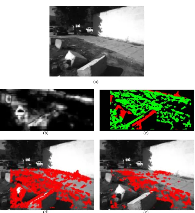
(a) (b)

(c) (d)

(e) (f)

(g) (h)

Figure 4.5: Obstacle detection results. (a): Left image acquired from a stereo camera and cropped to range r = 10m. (b): Saliency map computed from (a). (c-d) Graphical rep-resentation of the space-variant resolution for (a), using, in (c) the original method (EOD) [Santana et al., 2008] and in (d) the saliency modulated method (ESalOD) proposed in this dis-sertation. White pixels correspond to points that have been skipped by the detector due to the lack of saliency or computed range. Black pixels correspond to points that have been analysed. Note that, instead of analysing equidistant pixels (c), the method herein proposed (d) focus the analysis on salient regions and regions where obstacles are being detected, skipping more pixels, otherwise. This mechanism result in reduced computation, as less analysis are being made, and increased robustness, as analysis are focused in regions of interest. (e-h): Detected segments using the EOD’s space-variant resolution and the ESalOD’s space-variant resolution with the Voting Filter (section: 4.3) and Area Filter (section: 4.4.1) parameterised as follows: (e) EOD withv = 0anda = 0(f) ESalOD withv = 0anda = 0(g) EOD withv = 20and

(57)

Chapter 5 Hybrid Obstacle Detector

As stated in [Rankin et al., 2005], the variety of objects with different dominant techniques

presented in off-road environments requires the use of different detection techniques in parallel

for a complete detection of all possible obstacles.

This chapter presents a new obstacle detection architecture, represented in Fig. 5.1, that

integrates two different techniques in an efficient way, where saliency is used throughout the

system in order to reduce its computational cost and augment its robustness. Briefly, a coarser

and faster obstacle detector is used to detect large obstacles and to focus the a finer and slower

one on regions of the environment where small obstacles, and consequently harder to detect,

may be present. Detectors complementary role aims at the development of a system that

prop-erly trade-offs between computational cost and detection accuracy.

5.1 Architecture for Hybrid Obstacle Detection

The following describes the system in a nutshell. First, a stereo vision sensor provides two

images, one obtained from the left camera and another from the right one. The saliency map of

the left image is computed, and a stereo processing step is carried out in order to provide a dense

3-D points cloud [Konolige and Beymer, 2007]. Saliency information (see section 3.2) is then

(58)

SALIENCY COMPUTATION STEREO PROCESSING PLANE DETECTION OBSTACLES MAP ATTITUDE COMPENSATION SMALL OBSTACLES DETECTION RIGHT IMAGE LEFT IMAGE LARGE OBSTACLES DETECTION

-+ plane rotated 3-D point cloud large obstacles map small obstacles map saliency

map 3-D point 3-D point_cloud cloud plane saliency map large obstacles map extended saliency map

(59)

(a) image#6 (b) image#6

(c) image#7 (d) image#7

Figure 5.2: Hybrid Obstacle Detector results. In the left column are depicted the results for the small obstacles detector alone (as described in chapter 4 and set for its best parameterisation) and in the right column are depicted the results of hybridisation. Note the difficulty for the cone-based detector to classify the top of large homogeneous obstacles, which is resolved by its fusion with the plane based detector.

Subsequently, a large obstacles map is obtained by checking which 3-D points are considerably

above or below the ground plane. As the camera’s optical axis, normally, isn’t parallel to the

ground plane, the 3-D points are rotated according to the estimated ground plane and thus

compensating for the robot attitude. The large obstacles map is then subtracted from the saliency

one in order to focus the accurate obstacle detector (see Chapter 4) on areas that have not been

already analysed. Finally, the small and large obstacles maps are merged in order to produce

the final obstacles map.

Obstacle detection in all-terrain requires some adaptations to the process of computing

Vision Based Obstacle Detection for All-Terrain Robots

Magno Edgar da Silva Guedes

Vision Based Obstacle Detection

for All-Terrain Robots

UNIVERSIDADE NOVA DE LISBOA

Faculdade de Ciˆencias e Tecnologia

Departamento de Engenharia Electrot´ecnica

e de Computadores

Vision Based Obstacle Detection for All-Terrain Robots

Magno Edgar da Silva Guedes

Dissertação apresentada na Faculdade de Ciências e Tecnologia da

Universidade Nova de Lisboa para obtenc¸˜ao do grau de Mestre em

Engenharia Electrot´ecnica e de Computadores.

Orientador:

Prof. Jos´e Ant´onio Barata de Oliveira

Acknowledgements

Resumo

Abstract

List of Symbols and Notations

Contents

List of Figures

Chapter 1

Introduction

1.1

Problem Statement

1.2

Solution Prospect

1.3

Dissertation Outline

1.4

Further Readings

Chapter 2

State of the Art

2.1

Flat Terrain Assumption

2.2

OD in Terrains with Smooth Slope Variations

2.3

Traversability and Elevation Maps

λ

λ

λ

2.4

Statistic Analysis of 3-D Data

2.5

Geometrical Relationships in 3-D Point Clouds

2.6

Visual Attention Mechanisms

Chapter 3

Supporting Mechanisms

3.1

Stereo Vision

3.1.1

Disparity

3.2

Saliency Computation

3.3

Ground Plane Estimation

Chapter 4

Obstacle Detection Core

4.1

Obstacle Definition

4.2

OD Algorithm

4.2.1

Tilt-Roll Compensation

4.2.2

Space-Variant Resolution

4.3

Voting Filter

4.4

Obstacle Segmentation

4.4.1

Area Filter

Chapter 5

Hybrid Obstacle Detector

5.1

Architecture for Hybrid Obstacle Detection