2
Applied Economics Research | Center for Monetary StudiesYear 3 | Number 5 | March. 2015
SLOW GROWTH AND DEFLATIONARY FORCES: NO
SIGN OF RELIEF
1Debt overhang
Stability, euphoria, leverage and crisis
▀ We have long been taught that times in which the future of the economy is viewed with particularly great enthusiasm tend to give rise to substantial volumes of credit creation. Depending on how big the optimistic wave gets, both borrowers and lenders may go well beyond the points that prudence would recommend. This being the case, periods of euphoria may not end well. Financial crises and recessions will probably ensue.
The basic lessons on these matters were originally given by Charles Kindleberger and Hyman Minsky. (Kindleberger 1978; Minsky 1972 and [1986] 2008). Their books became classical ones.
In Minsky’s analysis, an extraordinarily optimistic wave usually arises in the wake of a stable macroeconomic scenario. In his words, “businessmen and bankers, heartened by success, tend to accept larger doses of debt-financing”. During periods of tranquil expansions, the argument continues, new financial instruments are created. “Full employment is a transitory state because speculation upon and experimentation with liability structures and novel financial assets will lead the economy to an investment boom. An investment boom leads to inflation and […] an inflationary boom leads to a financial structure that is conducive to financial crisis.” (Minsky, [1986] 2008, p. 199).
_1 The author wishes to thank Regis Bonelli and Fernando Veloso for reading the original version of this essay and making useful suggestions. A word of thanks is also due to Marcel Balassiano for his excellent research assistance.
3
Applied Economics Research | Center for Monetary StudiesYear 3 | Number 5 | March. 2015
Kindleberger described Minsky as “a monetary theorist who holds that the financial system is unstable, fragile, and prone to crisis.” (Kindleberger 1978, p. 8). He takes Minsky’s “model” as the starting point of his analysis. Events leading up to a crisis start with some sort of a displacement. “Whatever the source of the displacement – says the author -, if it is sufficiently large and pervasive, it will alter the economic outlook by changing profit opportunities in at least one important sector of the economy. […] If new opportunities dominate […], investment and production pick up. A boom is under way […] and is fed by an expansion of credit.” (Kindleberger, 1978, pp. 15-16).
After a time, the argument continues, increased demand presses against the economy’s productive capacity and the supply of existing financial assets. Rising prices attract new firms and investors. “At this stage we may get what Minsky calls ‘euphoria’ […] and Adam Smith and his contemporaries called ‘overtrading’. […] When the number of firms and households indulging in these practices grows large […] speculation for profits leads away from normal, rational behavior to what have been described as ‘manias’ or ‘bubbles’. The word ‘mania’ emphasizes the irrationality; ‘bubble’ foreshadows the bursting.” (Kindleberger, 1978, pp. 16-17). The most dramatic example of an economic contraction on record is of course the Great Depression. In its domestic (US) dimension, one of the first authors to investigate the essence of the problem was Charles Persons, who, writing when the crisis was still in its very beginning, associated the economic problems of that time to the excesses made in the 1920s. In doing so he made use of an approach entirely compatible with the theoretical framework later developed by Minsky and Kindleberger. In Persons’ words, “the existing depression was due essentially to the great wave of credit expansion in the past decade.” (Persons, 1930, p. 94).
At that time, aggregate information on the process of debt creation was not available, which led Persons to base his analysis on a rather incomplete set of data. The statistics he managed to gather involved information on the growth of bank loans and investments, mortgage debt, securities outstanding and installment credit. While credit grew rapidly in all of those fronts, particularly noteworthy was the fact that the 1920s saw a sort of a revolution in the way households acquired durable goods.
4
Applied Economics Research | Center for Monetary StudiesYear 3 | Number 5 | March. 2015
Installment financing became very common, contributing enormously to the rapid growth in sales and production. In Persons’ words, “rural districts and small cities are quite as familiar with down payments and monthly installments as are the largest cities. All income classes up to the richest have succumbed to the allurements of easy possession and ‘pay as you earn’”. (Persons, 1930, p. 109). Industries as diverse as those of furniture, clothing, electric appliances (refrigerators, washing machines, vacuum cleaners, sewing machines, radio), automobile and construction benefited a lot from the new arrangements.
All this might look desirable, noted the author, but “when every potential debtor and installment buyer has assumed the full burden of indebtedness which the new credit policies allow; when every would-be home owning family has purchased through the building and loan associations as costly a house as its resources will permit; and when every apartment house and business building has been burdened with as heavy a load of bonded indebtedness as the avid savers and investors can be persuaded to accept […] there is of necessity an end to the process.” (Persons, 1930, p. 120). As the process of expanding credit ceases, there is a return to a situation in which spending each year corresponds to no more than we earn that year. And “a painful period of readjustment” ensues. (Persons, 1930, p. 119).
Mistakes made by the producers of goods often aggravate the process. For a while, all they can produce they sell at profitable rates, a fact which urges them to expand their productive capacity. “When the check comes they find themselves with a great excess of productive capacity. Much investment funds are hopelessly sunk in idle plants.” (Persons, 1930, pp. 120-121). What happened to the radio industry (factories being closed or going on part time, stocks being sold at bargain prices, etc.) would be a particularly good illustration of this point. In sum, the check came, after we have temporarily “spent, enjoyed and stimulated business activity.” (Persons, 1930, p. 119).
The credit revolution that occurred in the US during the 1920s was also examined by Martha Olney. That period, she said, “mark the crucial turning point in the history of consumer credit. […] [As a percentage of household income], outstanding
5
Applied Economics Research | Center for Monetary StudiesYear 3 | Number 5 | March. 2015
nonmortgage consumer debt more than doubled in the 1920s.” (Olney, 1999, pp. 320-21).
In Olney’s analysis, it was the large drop in consumer spending what turned a minor recession into the Great Depression. “The collapse in consumption in 1930 came on the heels of a decade of virtual explosion in household use of installment credit”, she argued. (Olney, 1999, p. 320).
Peter Temin had already examined the 1930 fall in consumption. He considered it a truly autonomous movement, “too large to be easily explained”. (Temin, 1989, p. 43). Olney’s empirical investigation showed that “Temin’s autonomous drop in consumption essentially disappears when a role for debt is allowed”, a conclusion she arrived at by the introduction of a lagged debt variable into a regression analysis of nondurable consumption against real disposable income and real wealth. (Olney, 1999, pp. 330-31).
An interesting point in Olney’s analysis is her emphasis on the argument that decision to cut consumption in the presence of a heavy debt burden depends on the costs of default, that is, on its legal consequences. She argues that in the early 1930s defaulting was expensive, the reason being that, as down payments were normally large, durable goods acquired on credit usually embodied significant equity values, surpluses that consumers would lose in case they failed to meet their financial obligations, triggering repossessions. Thus, in order to avoid default, and pressed by the adverse economic situation (the US was in recession since the third quarter of 1929), indebted households opted for reducing consumption. Later, when the economy experienced another recession (1937-38), institutional arrangements had changed, substantially reducing the cost of default. As a result, a higher proportion of indebted households chose to default rather reduce spending.
Decades later, in the early 1990s, many industrialized economies went through protracted periods of slow growth. Some of them suffered the longest recessions since the 1930s. And again the question of private-sector indebtedness was present. According to Mervyn King, the most severe recessions “occurred in those countries which had experienced the largest increases in private debt burdens”. (King, 1994, pp. 419-420).
6
Applied Economics Research | Center for Monetary StudiesYear 3 | Number 5 | March. 2015
Based on a sample of ten major economies, the G7 plus Australia, Norway and Sweden, King’s exercise revealed a good correlation between the difference between the actual annual growth rate observed in the 1989-92 period and the trend growth rate (measured by average GDP growth rate between 1974 and 1989), on the one hand, and the change in the household debt to GDP ratio from 1984 to the end of 1988, on the other. The larger the rise in household debt, the worse the growth performance. (King, 1994, p. 420).
Household indebtedness affects the economy through the behavior of family consumption. Examining the UK experience during that time, King noticed that consumption had shrunk more than in previous recessions. “Aggregate consumption fell for seven consecutive quarters and by 3.5% from peak to trough, a period in which real disposable income rose by 1.1%.” (King, 1994, p. 424). Recalling the importance of mortgages in total household debt, the author compared the behavior of consumption between two groups of home-owners. He found that, between 1989 and 1991, total real consumption expenditure of households with a mortgage fell by approximately 2.0%, whereas the consumption of those without a mortgage rose by almost 4.0%. And that real non-housing expenditure fell by more than 4.0% for home-owners with a mortgage and rose by 1.0% for those with no mortgage debt. These and other evidences allowed the author to conclude that there was “a prima facie case for thinking that high debt burdens, especially the increase during the 1980s, led to a deeper and longer recession than might otherwise have occurred.” (King, 1994, p. 426).
The Japanese experience
In the second half of the 1980s, a particularly significant episode of rapid credit creation was that of Japan. To some extent, this was due to the expansionary monetary policy followed by the Bank of Japan as part of the international policy coordination program agreed to by members of the G5 under the Plaza Accord in September 1985. The idea of the meeting was to find means of putting an end to the long cycle of dollar strengthening observed for approximately six years. At the time,
7
Applied Economics Research | Center for Monetary StudiesYear 3 | Number 5 | March. 2015
the US current account was in deficit. Germany and Japan had surpluses. The imbalances should be corrected and for that to happen an “orderly appreciation of the main non-dollar currencies against the dollar” was considered desirable.
On the eve of the Plaza meeting the Japanese currency was quoted at 240 yens per dollar. On the first day of January 1986 the rate was 200. In May it reached 160. The pace of appreciation diminished from that point onward, but the tendency continued. At the final day of 1987 the rate was 120 yens per dollar.
The expansionary monetary policy adopted by the Bank of Japan was part of the country’s commitment to stimulate the economy and would probably more than compensate for the contractionary impact of the strengthened yen. Between January 1986 and February 1987, in five movements of 50 basis points, the official discount rate was lowered from 5.0% to 2.5% per annum.
Helped by a deregulation program, the monetary stimulus led to strong credit expansion, which occurred not only through the banking system but also through the capital markets. Between early 1987 and the end of 1990, the stock of bank credit, for example, went up by 60%. Economic activity increased considerably. The GDP annual growth rate, which had fallen from 6.3% in 1985 to 2.8% in the following year (due largely to the strengthening of the yen), reached 4.1% in 1987 and an average of 6.0% in 1988 through 1990.
Asset prices skyrocketed. The stock market peaked at December 1989, while the same happened to land prices a few months later (September 1990). From early 1985 until the corresponding peaks, the Nikkei 225 went up by 222% and the Urban Land Price Index (commercial areas, six major cities) rose by 308%. Both indexes never recovered from their collapses. In a matter of 32 months, the Nikkei 225 had fallen almost 60%. Further weakened, in April 2003 the stock market index corresponded to something like 20% of its historical peak. That percentage is presently around 47%. As to the land price index, it has declined systematically since 1990, except for the three to four years which preceded the 2008 world crisis. Nowadays, it corresponds to approximately 15% of its historical peak. Notice that the official discount rate, maintained at the 2.5% level between early 1987 and May 1989, had gone up to 6.0%
8
Applied Economics Research | Center for Monetary StudiesYear 3 | Number 5 | March. 2015
in August 1990, a movement which probably contributed to the bursting of the bubble.
The loss of wealth caused by falling land and stock prices was dramatic. It corresponded to three years of Japanese GDP, the greatest economic loss ever experienced by a nation in peacetime, noted Richard Koo. (Koo, 2009, p. 16). Since Japanese firms were usually highly leveraged, as the value of properties collapsed their balance sheets suffered a tremendous impact. Many went underwater, although their products continued being strongly demanded by consumers. In general, cash flows and profits remained robust.
Koo argues that when this happens firms begin to shift their priority from profit maximization to debt minimization – in case excess debt is accumulated by households, they behave similarly. Repairing the balance sheets becomes the main objective. This produces an economic outcome which differs considerably from an ordinary recession. (Koo, 2009, pp. 14-15, 85). He called it a balance sheet recession. For Koo, what causes such a phenomenon is the changed behavior of private economic agents (basically firms in the case of Japan) in response to the damage inflicted to their net worth. Based on a flow of funds analysis, Koo argues that Japanese firms began shifting their priorities to debt minimization around 1993. Since then, the number of companies paying down debt increased constantly. By 1998 the corporate sector as a whole had become a net saver. Two more years and businesses were saving more than households. As business behaved this way, demand contracted considerably. (Koo, 2009, pp. 22 and 90).
Economic growth in Japan was very weak in 1992 through 1994 (average of 0.6% per year). Since then it oscillated substantially, but its average (0.9% in 1995-2014) never returned to the level observed in previous decades – average growth had been 4.2% in the 1970s and 80s, and more than 10% in the 1960s. The very low rates of growth observed in 1992-94 led the Bank of Japan (BOJ) to aggressively lower the basic interest rate, until it reached 0.5% per annum in September 1995. Since then, except for a brief period during which it was set at 0.5%, it has been systematically below that level.
9
Applied Economics Research | Center for Monetary StudiesYear 3 | Number 5 | March. 2015
In response to the renewed weakness of the economic performance observed in the late 1990s and early 2000s, the Bank of Japan resorted to an unprecedented monetary policy experiment, usually referred to as “quantitative easing” (QE). The QE program lasted from March 2001 to March 2006, a period during which the basic interest rate declined further, to practically zero. At that time, the BOJ was particularly concerned with the behavior of inflation, which had entered into negative territory in the final years of the 1990s.
While the BOJ had announced that the practically zero interest rate policy (ZIRP) would be maintained until the “deflationary concern was dispelled”, as the QE program was launched they made a stronger commitment. Now it was linked to the track record of the CPI. More specifically, the policy would last until the CPI (excluding perishables) stabilized at zero percent or showed an increase year on year. Besides this, the program involved two more pillars. First, the BOJ replaced the overnight call rate by the outstanding current account balance (CABs) held by financial institutions at the Bank as the main operating target for money market operations. The target established for the CABs was raised considerably until 2004, reaching levels several times higher than the size of required reserves. Liquidity would be provided by the monetary authority to assure the meeting of the target. Second, the BOJ would purchase long-term Japanese government bonds, thereby changing the composition of the Bank’s balance sheet.
A considerable improvement in economic activity was what led to the abandonment of QE. From 0.35% in 2001-02, the average GDP growth rate had gone up to 1.8% in 2003-05. The recovery lasted until the beginning of the Great Recession, with 2006 and 2007 being years of particularly good performance (average growth around 2.0%). Measured by the CPI (ex-fresh food), the inflation rate turned slightly positive in 2005, after being in the negative territory since 1998.
In general, analysts do not find anything more than a limited impact of QE, which is equivalent to saying that probably the program did not constitute a major factor behind the economic recovery. In any case, however small that impact might have been, it seems that the channel through which QE produced some result was related to its influence on the expected future path of short-term interest rates.
10
Applied Economics Research | Center for Monetary StudiesYear 3 | Number 5 | March. 2015
Richard Koo argues that QE would have worked if the tremendous increase in bank reserves had somehow boosted the money supply through the creation of credit by the banking system - in the 1970s and the 1980s, for example, the monetary base, credit and the money supply had grown hand in hand. But this is not what we saw during the QE period, due to the absence of willing private borrowers. Notice that the paying down of debt by private economic agents causes a decline in the stock of loans and the money supply, contractions that can be neutralized (at least partially) by government actions in the opposite direction, that is, by government borrowing. In reality, a partial compensation is exactly what happened in Japan, as indicated by the behavior of certain monetary aggregates: during the QE period, the monetary base went up by 61% while the means of payment (M2) rose by 10.5%. Japan’s money supply would have contracted had it not been for an increase in government borrowing. According to Koo, during the US Great Depression, “the US money supply shrank by 33 percent as businesses and households drew down their bank deposits to pay back loans”, giving rise to a deflationary spiral. (Koo, 2009, pp. 31-33).
In the author’s opinion, the recovery had to do with the fact that around the mid-2000s companies had repaired their balance sheets and were starting to invest the cash flow they had been using to pay down debt, and because exports were growing, “both factors entirely unrelated to the Bank of Japan’s supply of liquidity”. (Koo, 2009, p. 74).
For those who claim that the long Japanese recession had to do with problems in the banking sector, Koo has a convincing argument. In his words, “if banks had been the bottleneck […] we should have observed several phenomena that are typical of credit crunches.” (Koo, 2009, p. 7). First, if companies were unable to borrow from banks, they could have issued debt or equity securities on the capital markets. Second, if Japanese banks were stuck with bad loans, foreign banks would have expanded their loans to business. Third, if banks were constrained in their ability to lend, lending interest rates would have risen. “But nothing remotely like this happened in Japan”, he says. (Koo, 2009, p. 9).
11
Applied Economics Research | Center for Monetary StudiesYear 3 | Number 5 | March. 2015
In short, Koo argues that the recession was long because corporate balance sheets were dramatically affected by the collapse of asset prices. As a result firms changed their priority and started being concerned with repairing the damage. As they increasingly opted for paying down their debt, the corporate sector as a whole eventually became a net saver. Interest rates close to zero did not become a strong enough force to change that behavior. As demand from the private sector contracted, the economy suffered. Koo argues that from a given point onward, the government became the only borrower, a fact which contributed to the growth of the money supply. Were it not for the fact that the government continued to borrow and spend, the argument continues, Japan would have experienced a depression. (Koo, 2009, pp. 25-26 and 34).
Koo draws an analogy between Japan’s Great Recession and the US Great Depression. He stresses the fact that in the US both households and firms had borrowed too much during the 1920s. According to his analysis, the US depression was also a balance sheet recession, triggered by the private sector striving to minimize debt. In Japan as well as in the US, the major problem was “a lack of demand for loans in the private sector”, which directly affected the money supply and aggregate demand. In his opinion, it was not a problem of lack of funds supplied by the monetary authorities, as most researchers had concluded. (Koo, 2009, p. xiv and pp. 85-104). “Economists incorrectly assumed that the liquidity trap was a lender-side phenomenon, when it was actually a borrower-side phenomenon”, he said. (Koo, 2009, p. 109).
The Great Recession
The recession which followed the recent financial crisis, known as the Great Recession, is another important illustration of the idea that crises tend to occur in the wake of periods of excessive enthusiasm. In that case, several factors seem to have worked in the same direction, at the same time, contributing in their own way to the rapid expansion of credit and the formation of asset-price bubbles in the US and other countries.
12
Applied Economics Research | Center for Monetary StudiesYear 3 | Number 5 | March. 2015
To begin with, we must notice that the increased degree of financial and trade integration, made possible by deregulation and rapid rates of technological progress, facilitated the international transmission of economic and financial events from one country to another.
We must also recall that the period going from the mid-1980s to the beginning of the crisis became known as the Great Moderation, due to the fact that, particularly in the US and in comparison to previous episodes, recessions had become a much milder and less frequent phenomenon, while inflation rates had stabilized at low levels. In other words, the period was marked by a considerable decline in the volatility of inflation as well as of output and employment, a fact which led many to believe that the economic cycle had been tamed.
In a book published in 2009, John Taylor argued that “monetary excesses were the main cause” of the boom and resulting bust of the housing sector in the US. (Taylor, 2009, p. 1). His argument is based on the fact that, between 2002 and early 2006, worried about the possibility of deflation, the Fed had set the policy rate at levels substantially below the ones which would have prevailed if the monetary authorities had not abandoned the historically observed pattern, supposedly given by the so-called Taylor rule.
For sure, it would be too simplistic to attribute the crisis to the apparent mismanagement of monetary policy in the US, with its spillover effects on the rest of the world economy. A major event like that cannot have a single cause. Additionally, one of the most relevant aspects of the discussion on the secular stagnation hypothesis, revived by Larry Summers, has to do with the possibility that in the years prior to the crisis the world economy might have gone through considerable structural change, which became more visible after the crisis, but had already produced a significant decline in the equilibrium real rate of interest, supposedly determined by the interaction of international forces. (Summers, 2013).
To the extent that the hypothesis raised by Summers is a valid one, the monetary authorities face a dilemma. Lowering the policy rates would stimulate the formation of bubbles and a borrowing spree, but it would probably contribute to the maintenance of the growth process, without significant inflation. In case the central
13
Applied Economics Research | Center for Monetary StudiesYear 3 | Number 5 | March. 2015
banks – particularly the Fed – refused to follow what seemed to be a declining trend of the equilibrium real rate of interest, it would have hurt the growth process and probably allowed for undesirable deflationary pressures. This seems to be the gist of the message sent by Summers. Structural changes made it difficult for industrial economies to achieve full employment, economic growth and financial stability at the same time. (Senna, 2015, chapter 4).
With no intention of exhausting the list of factors behind the Great Recession, we can add that the creation of the euro also contributed to the widespread optimistic wave which preceded the crisis. In fact, the new currency brought about a great deal of enthusiasm, best illustrated by the extraordinary convergence of interest rates across the region. Governments which used to pay a lot more than the Germans to access the financial markets suddenly found themselves obtaining funds at rates very close to those paid by the most reliable issuer in the zone. As the rates on securities issued by several member countries declined, so did interest rates in general. In the so-called periphery, the dominant sentiment was that a passport to prosperity had just been acquired.
In a rather unavoidable way, private debt started to climb. Households, firms and banks simply jumped at the opportunity to borrow under conditions never seen before. The disappearance of the exchange-rate risk within the area stimulated the borrowing spree, while banks in the center of the region felt encouraged to substantially increase international lending within the zone.
On the monetary side, the one-size-fits-all policy gave extra impulse to the new spending cycle. In fact, soon after the introduction of the euro, the German economy was not in a position to support high rates of interest (economic performance was weak from 2001 until the beginning of 2005), while a great deal of enthusiasm prevailed in the periphery. The German situation and perhaps the low levels of interest rates observed in the international markets, particularly in the US, led the European Central Bank to lower its policy rate, from 4.5% on April/01 to 2.0% in June/03, a level which prevailed until the end of 2005. Given the circumstances, the basic interest rate became negative in real terms for a varying number of years in Greece, Portugal, Ireland, Italy and Spain. While the major economic problems in
14
Applied Economics Research | Center for Monetary StudiesYear 3 | Number 5 | March. 2015
Greece had more to do with mismanagement of the fiscal accounts, in Portugal, Ireland and Spain the whole scenario produced an extraordinary increase in private leverage and debt. In Ireland and Spain this was accompanied by housing booms. As regards the empirical evidence on what happened in the years before and immediately after the recent financial crisis, it is worth noting the results obtained by Glick and Lansing (Glick-Lansing, 2010). Their study illustrates the rapid rise of household borrowing in the US and in many industrial economies in the years leading up to the financial crisis. The authors showed that countries exhibiting the largest increases in household leverage (measured by the ratio between household debt and disposable income including transfers) from 1997 to 2007 also tended to experience the fastest rise in house prices over the same period. “The pattern suggests that the link between easy mortgage credit and rising house prices held on a global scale.” (Glick-Lansing, 2010, p. 3).
In addition, the authors found that countries experiencing the largest increases in household leverage before the crisis tended to be those which suffered the most severe recessions – the measure of severity was the percentage decline in real consumption from the second quarter of 2008 to the first quarter of 2009. In the end, they expressed the concern that, in many countries, efforts of households to reduce their elevated debt load via increased saving might result in sluggish recoveries of consumer spending. (Glick-Lansing, 2010, p. 4).
Based on the performance of advanced economies over a period of three decades, a study published as chapter 3 of the April 2012 World Economic Outlook (IMF) gave further support to the idea that “housing busts preceded by larger run-ups in gross household debt are associated with deeper slumps, weaker recoveries, and more pronounced household deleveraging.” (IMF, 2012, p. 115).
We can thus say that theoretical considerations and important empirical evidence suggest that recovery from financial crises requires a correction of the excesses of the past. In other words, deleveraging is pre-condition for the resumption of sound economic growth.
15
Applied Economics Research | Center for Monetary StudiesYear 3 | Number 5 | March. 2015
Deleveraging?
Still in regard to the Great Recession, it is widely known that, with few exceptions (notably Greece), the initial run-up in debt had its origin in the private sector, particularly households and banks. As Paul De Grauwe has shown, prior to 2008, in several European countries, for example, government debt ratios were declining, sometimes in a very significant way. (De Grauwe, 2010). But the seriousness of the worldwide financial crisis forced central governments to intervene, in different forms. In general, there were initiatives taken in support of the banking industry and substantial increases in government expenditures, to compensate for employment losses and weaker economic activity. Inevitably, official debt levels went considerably up.
As previously discussed, excess leverage tends to inhibit private expenses. This seems to be true for both households and firms. But what about government leverage? Would it be fair to say that high levels of public debt are also capable of inhibiting private expenditures?
The answer to this last question is probably yes. High public debt ratios may be seen as a source of risk or uncertainty. In the presence of high public debt, private economic agents usually fear future adjustments. They normally imagine that at some point down the road some sort of a correction will take place, involving, for example, expenditure cuts, higher taxes, or even something more drastic, like default or an inflationary explosion.
An important study on leverage came out in September last year. The authors show that, for the world economy as a whole, total debt ex-financials went up from a little more than 160% in 2001 to almost 215% of the GDP in 2013. During this period, the ratio went up year after year. In 2009 it moved up at a rate considerably faster than before, as government debt rose abruptly. Since then the global debt to GDP ratio continued to grow, particularly due to what happened in emerging economies. In the group of developed nations the rate of growth diminished substantially, but remained positive. The conclusion is that, in the aggregate, we can say that deleveraging has not started yet. (Buttiglione et all, 2014, pp. 11-17).
16
Applied Economics Research | Center for Monetary StudiesYear 3 | Number 5 | March. 2015
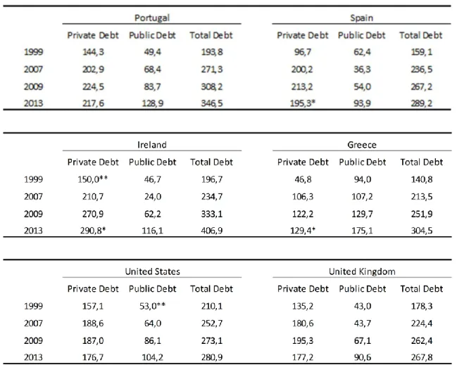
Table 1: Total Debt (% of GDP) - Selected Countries
Note: *data of 2012; ** data of 2001. Total debt = private debt + public debt; private debt = non-financial corporations + households; public debt = general government gross debt. Sources: OECD, IMF and Federal Reserve.
Table 1 shows the behavior of the debt to GDP ratio in selected economies. A breakdown is presented between private (ex-financials) and public debt. In no country in the sample has the ratio declined from the high levels of total debt reached in 2009. In fact, the opposite is true, that is, the ratio has gone further up. In four cases, we observe some deleveraging in the private sector, but it should be noticed that, in spite of this movement, societies were still significantly more indebted in 2013 than in 1999, for example.
17
Applied Economics Research | Center for Monetary StudiesYear 3 | Number 5 | March. 2015
An asymmetric adjustment in the Eurozone
Between the early 1870s and the beginning of World War I, and again during the interwar period, a large number of developed economies in the Western world operated under the so-called international gold standard. Under that system, domestic currencies were convertible and had fixed parities to the gold. Policymakers’ number-one priority was to maintain those parities.
It is widely believed that the gold standard embodied a deflationary bias. Such belief has to do with the fact that the system did not work as smoothly as it was supposed to do. The basic idea governing the functioning of the system was that disequilibrium situations would be corrected by means of the so-called price-specie-flow mechanism. Under such mechanism, a country in deficit (due to loss of competitiveness, for example) would suffer a drain in international reserves, while the rest of the world would gain reserves. The contraction in the domestic money supply would exert a downward pressure on the domestic price level, while the expansion in the money supply would do the opposite elsewhere. Prices would tend to fall internally and to go up abroad. After a while, the flow of reserves would come to an end and equilibrium would be restored.
In theory, the system could count not only on such automatic mechanism but also on measures discretionarily taken to accelerate the adjustment. Policy makers in the deficit country - where reserves were being drained and the money supply contracted – would sell domestic financial assets, lowering their prices and pushing interest rates further up, thereby provoking an additional monetary contraction. Countries in surplus would acquire financial assets, pushing up their prices and lowering interest rates, reinforcing monetary growth. Those who acted this way were said to play by the “rules of the game”.
Adherence to those rules was a form of cooperation. The problem was that incentives to cooperate were not symmetrical. Authorities were much more inclined to act according to the rules when facing deficits than in the presence of surpluses, the reason being the disproportionally high potential costs associated with the possibility
18
Applied Economics Research | Center for Monetary StudiesYear 3 | Number 5 | March. 2015
of losing reserves to the point of making convertibility unsustainable. (Senna, 2010, pp. 68-71).
It is interesting to notice that countries in surplus could not only refrain from giving further impetus to the expansion of the money supply but could do exactly the opposite. By acting this way they were said to be “sterilizing” the influx of reserves. Rather than buying financial assets they would sell them, thereby neutralizing the effects of gold inflows.
In their A Monetary History of the United States, Milton Friedman and Anna Schwartz showed that during the 1920s the Federal Reserve made intense use of the sterilization mechanism. “From 1923 on, gold movements were largely offset by movements in Federal Reserve credit so that there was essentially no relation between the movements in gold and in the total of high-powered money”, they said. (Friedman-Schwartz, p. 282). To the extent that surplus countries acted in this manner, and recalling the countries in deficit had little or no option, we can say that the burden of the adjustment was left on the shoulders of this last group, thereby creating a deflationary bias.
This line of reasoning is certainly correct under ordinary circumstances, but it is worth noting that Richard Koo questions its validity as an explanatory factor of the Great Depression in the US. Let us consider, for example, what happens in a surplus country. In order to inflate such an economy, it is necessary not only that there is no break in the relation between the inflow of gold and the expansion of high-powered money (the monetary base), but also no break in the relation between high-powered money and the money supply (means of payment) as well. Koo argues that even if the Fed had allowed the monetary base to expand (that is, avoided sterilization), the money supply would not have expanded. In reality, it would have contracted, since this is exactly what happens when economic agents are paying down debt. In Koo’s opinion, when demand for funds is shrinking fast, “whether gold is coming in or out of the country is largely irrelevant”. The key driver of the Great Depression was private-sector debt repayment, “which torpedoed both the money supply and aggregate demand. The resultant deflationary spiral was impervious to monetary
19
Applied Economics Research | Center for Monetary StudiesYear 3 | Number 5 | March. 2015
easing, because the highly leveraged private sector was desperately minimizing debt.” (Koo, 2009, pp. 108-109).
When we think about what happened in the Eurozone in recent years we cannot avoid recalling the working of the old gold standard. In fact, the world represented by the present euro area and the group of economies which were integrated under the gold standard have important things in common: a) in both cases, member countries opted for not having the exchange rate as an adjustment instrument; b) preserving the system supposedly became an important goal; and c) in the presence of external disequilibrium, cooperation among members is extremely useful.
As discussed earlier, the creation of the euro was itself a source of enthusiasm, at least for countries in the periphery. Interest-rate spreads over the German bunds practically disappeared. With the exception of Italy, peripheral economies experienced an extraordinary rise in private spending and leverage. Inevitably, this had consequences for the balance of payments. Current account deficits increased to very high levels. In Greece, for example, the disequilibrium went up from 5.4% of the GDP to 15.0%, in the ten-year period to 2008. In Portugal, Spain and Ireland, the corresponding movements were from 8.7% to 12.6%, from 2.9% to 9.6%, and from 0.2% to 5.7%, respectively. During the same period, Germany followed the opposite path, going from a deficit equivalent to 1.5% to a surplus of 6.0% of the GDP.
As the crisis heavily hit the peripheral countries, they were forced to adjust by those in command of financial help. Adjustment meant tight fiscal policies, the only macro instrument they were left with after the creation of the euro. As expected, restraints imposed on demand expansion contributed to the correction of external disequilibria. Graph 1 illustrates the adjustment path followed by Greece, Portugal, Spain and Ireland. The current account of all these countries turned into positive territory. In the same graph it can be seen that the surplus observed in Germany in 2014 was approximately 7.0% of the GDP, that is, higher than the 6% registered in 2008.
20
Applied Economics Research | Center for Monetary StudiesYear 3 | Number 5 | March. 2015
Graph 1: Current Account (% of GDP) in Eurozone´s Periphery Countries
Source: IMF.
What this analysis indicates is that the burden of the adjustment has been basically borne by the countries which had experienced increasing external deficits in the years leading up to the crisis. The absence of cooperation, regarding the adjustment process, created a deflationary bias. (De Grauwe, 2015).
Stagnant real wages in advanced economies
Household consumption is generally the dominant component of aggregate demand. And wages usually represent the most important source of household income. This means that those concerned with the behavior of aggregate demand should have a great interest in understanding what is happening to the performance of real wages. A recent research sponsored by the International Labor Organization (ILO) shows that, in the developed world, real wages have been lagging behind productivity growth since 1999. (ILO, 2015). Why is it that even before the crisis wages were already growing at a relatively slow pace? The reasons for this are not completely clear, but they are probably related to competition from China, the diminished power of labor unions (induced or not by that competition) and a sort of a generalized
21
Applied Economics Research | Center for Monetary StudiesYear 3 | Number 5 | March. 2015
Graph 2: Labour Productivity Index and Real Wage in Advanced Economies
Note: Wage growth is calculated as a weighted average of year-on-year growth in average monthly real wages in 36 economies;
labour productivity refers to GDP (output) per worker; index: 1999 = 100. Sources: ILO Global Wage Database (figure 7) and ILO Trends Econometric Models, Apr. 2014.
abandonment of minimum-wage policies. Judging by the evidence provided by the ILO study, the gap between real wages and productivity widened after the crisis. The investigation covers a sample of 36 countries and productivity is defined as GDP per worker. The results are reproduced in graph 2.
Real wages have been practically stagnant in recent years. However, one cannot be fully confident that this constitutes a factor which is clearly contributing to the weakness of consumption expansion in the advanced world. After all, not only household expenditures are affected by real wages. Other components of aggregate demand are affected as well. Exports, for example, can be pretty much influenced by that variable. Countries facing a serious external disequilibrium often work towards restraining wage growth, in order to restore competitiveness. The net impact on aggregate demand depends on the relative importance of the partial influences on consumption, exports and investments as well.
In spite of the relevance of these considerations, it seems that one is safe enough to
assume that the present situation of stagnant real wages is an important factor22
Applied Economics Research | Center for Monetary StudiesYear 3 | Number 5 | March. 2015
contributing to the weak performance of household consumption in the developed world. Were it not for such belief, Germany would not have approved a new minimum-wage policy (effective 2015) and Japanese and American authorities would not be encouraging companies to increase basic pay, with support from the IMF. (ILO, 2015, p. 2).
Deflationary forces
So far we have discussed some important factors which have probably contributed to sluggish economic growth in the advanced world in recent years. For sure it is not our intention to exhaust the list of possibilities. For our purposes here, it suffices to make a brief comment on another element, generally known by the expression secular stagnation.
This possibility was examined by us in the September 2014 issue of this Monetary Policy Monitor, later reproduced as chapter 4 of our Essays and Conversations on Monetary Policy. (Senna, 2015). Associated with the name of the economist Larry Summers, the theory is essentially an attempt to explain an observed weakening of aggregate demand, the first signs of which had already appeared in the pre-crisis period. The basic idea behind it is that important structural changes – namely, an increase in the propensity to save and a diminished demand for investments - had occurred in the industrial world. As a result, aggregate demand contracted and the equilibrium real rate of interest (globally determined) fell. Since central bankers usually conduct monetary policy with an eye on the equilibrium (or neutral) real rate, they felt compelled to lower their policy rates, a movement which certainly contributed to the increase in leverage and the formation of bubbles in the running up to the crisis. According to this reasoning, the lowering of the policy rates was meant to compensate for the negative impact of the mentioned structural changes. Were it not for that action, economic growth would have been quite poorer than it actually was. More than six years into the post-crisis period, it seems that the secular stagnation hypothesis is an idea that will not abandon us soon. This point is well
23
Applied Economics Research | Center for Monetary StudiesYear 3 | Number 5 | March. 2015
illustrated by the fact that this was the theme of the first posts by Ben Bernanke on his new blog. (Bernanke, 2015).
In a recent article on the same subject of the present essay, Lo and Rogoff examined a larger number of factors, and concluded that it is too soon to have a strong opinion on the validity of the various theories. “One reason it is too soon to sort out the alternative viewpoints is simply that the pace of deleveraging remains modest or non-existent in many sectors around the global economy, implying that the debt overhang may still be a significant impediment.” (Lo-Rogoff, 2015, p. 15).
Independently from the validity of the different theories, the fact of the matter is that the world economy is experiencing important deflationary pressures. In China, the Eurozone and the UK wholesale-price inflation has been running in negative territory for more than three years, approximately two and almost one year, respectively. In the US the rate of inflation became negative in December 2014, reaching minus 7.1% (YoY) in February 2015.
At the consumer level, inflation rates (on a yearly basis) in those parts of the world are close to zero in the UK and the Eurozone, slightly positive in the US (measured by the PCE), and 1.4% in China. This downward trend has been heavily influenced by declining energy prices, but it is noticeable on a core basis as well, at least in two of those areas (the UK and the Eurozone).
If we look at import-price indexes, they are heading downward since the second semester of 2014 in the US, the UK and the European Union (we did not find information for the Eurozone), having reached the following annual rates of change: -10.5%, -6.9% and –3.1%, respectively. In China, import-price inflation has been around zero since October 2012.
Inevitably, those deflationary forces have affected the level of nominal interest rates. At the closing of March 2015, for example, the 10-year rates on government bonds were 0.2% in Germany, 1.6% in the UK and 1.9% in the US. These rates clearly suggest that economic agents expect the low-inflation environment to last for several more years.
24
Applied Economics Research | Center for Monetary StudiesYear 3 | Number 5 | March. 2015
An unbalanced economic recovery
The American economy is widely recognized as quite flexible. Even during the acute phase of global financial crisis (GFC), and in spite of the fact that it was at the epicenter of the crisis, it was common to hear that the US would be the first country to come out of the woods, a possibility which would certainly have important implications for the external value of the dollar.
Such a prediction is proving correct. As indicated at an earlier point, the US is one of the countries in which some deleveraging of the private sector is under way, a movement which clearly contributes positively for the recovery.
Independently from the magnitude of that contribution, the fact is that the US is well ahead of other major areas of the world economy, particularly Japan and the Eurozone. To begin with, in the final quarter of 2014, real GDP in the US was 8.7% higher than in the last quarter of 2007, for example, characterizing a real recovery. In contrast, Japan and the Eurozone still operated below the end-of-2007 level, more specifically 0.3% and 1.3% below.
Recently, in the last three quarters, Japan experienced negative rates of growth and the Eurozone grew at a pace of 0.8% (average of year-on-year rates). In the US, the average rate of expansion in the last three quarters was 2.6%.
Economic growth usually amplifies economic opportunities. It is reasonable to assume, then, that the above-illustrated difference in economic performance means that the US economy has had more to offer in terms of investment opportunities than her main competitors, this being the main reason why the dollar has appreciated so significantly in recent times. Graph 3 shows the behavior of the American currency in the international markets since the adoption of the flexible exchange-rate regime in the early 1970s. We can notice that the panic that accompanied the acute phase of the GFC brought about a significant rise in the value of dollar against the basket of major currencies represented by the dollar index, but that was a short-lived movement. In contrast, from August 2011, when the index reached its lowest historical point, to March 2015 (a period of three and a half years) the dollar has strengthened by 32.8%.
25
Applied Economics Research | Center for Monetary StudiesYear 3 | Number 5 | March. 2015
The same graph allows us to see that the exchange-rate cycles tend to be long. On average, upward and downward trends last approximately a little more than seven years. This in itself suggests that the present cycle has more to go. But what about the “fundamental” factors behind the process? If our analysis is correct, that is, if the dollar has strengthened due to the better economic performance exhibited by the American economy, any attempt to visualize if there is room for further appreciation of the dollar requires drawing a perspective on the relative growth performance of the US economy. To the extent that the Americans continue to outperform their main competitors, it is fair to assume that the dollar will experience further appreciation.
Independently from the impact of the observed deceleration of economic growth in China on the dollar price of certain commodities, when the dollar rises, the price of commodities quoted in the American currency tends to fall – since producers face costs in local currencies, a rising dollar leaves room for reduction in the dollar prices. This inverse relationship may not be valid for each and every commodity, but it seems to hold in the aggregate. Of course, for this to be one more element adding to the deflationary forces we are talking about, the fall in the dollar price of commodities
Graph 3: Dollar Index Since 1973
Note: Major currencies index includes the Euro Area, Canada, Japan, United Kingdom, Switzerland, Australia, and Sweden; March 1973 = 100; monthly averages. Source: Federal Reserve.
26
Applied Economics Research | Center for Monetary StudiesYear 3 | Number 5 | March. 2015
has to be stronger than the impact of the depreciation of domestic currencies against the dollar on local prices.
Quantitative easing
As discussed above, the bursting of bubbles formed in the final part of the 1980s led to a dramatic decline in economic activity in Japan in the first years of the ensuing decade. The economy experienced a recovery from 1994 onward but suffered two consecutive years of economic contraction in the wake of the Asian crisis (1998-99). At that time, a deflationary process got under way. A few years into this process and the Bank of Japan decided to resort to the quantitative easing experiment (QE), a program which lasted until inflation turned slightly positive in 2005. Inflation went up until it reached 1.0% per annum in 2008, but became negative again as the economy contracted once more (again for two consecutive years), this time in consequence of the beginning of the Great Recession. Measured by the consumer price index (ex-fresh food), the inflation rate was -1.7% in 2009, -0.5% in the following year, and stayed slightly below zero in 2011-12.
In mid-December 2012, Shinzo Abe led his party (the LDP) to the victory in a general election. He soon announced the three “arrows” of an economic strategy which became known as “Abenomics”. The strategy involved: a) a bold monetary accommodation by the Bank of Japan (BoJ); b) additional fiscal stimulus; and c) structural reforms. The objective of the new economic policy was to put an end to practically twenty years of slow growth and a deflationary environment. Prime-Minister Abe instructed the BoJ to pursue a 2% per annum inflation target.
On April 4, 2013, Haruhiko Kuroda, the newly appointed head of the BoJ, launched an aggressive monetary accommodation program called “quantitative and qualitative easing” (QQE), with the following characteristics: a) the BoJ will “double the monetary base” in two years; b) the target of 2% year-on-year rate of CPI inflation will be achieved “at the earliest possible time, with a time horizon of about two year”; c) the operating target for money market operations will change from “the uncollateralized overnight call rate to the monetary base”; and d) “with a view to
27
Applied Economics Research | Center for Monetary StudiesYear 3 | Number 5 | March. 2015
encouraging a further decline in interest rates across the yield curve, the Bank will purchase JGBs so that their amount outstanding will increase at an annual pace of about 50 trillion”. The official communique ended by stating that the measures would contribute to raise inflation expectations and would “lead Japan’s economy to overcome deflation that has lasted for nearly 15 years”.
In his most recent book, Richard Koo calls attention for the not-so-great enthusiasm with which the new monetary policy was received in Japan. In fact, as noted earlier, the economy had already gone through a similar program – between 2001 and 2006, the first time a central bank deliberately increased the stock of high-powered money with the purpose of raising inflation - with no visible positive result. Furthermore, as Kuroda announced his program, liquidity was already being deliberately expanded and the monetary base to GDP ratio was already considerably higher in Japan than in countries which had gone through comparable experiences (the US, the UK and the Eurozone), something that can in part be explained by a cultural factor, more specifically, the fact that cash is used much more intensively in Japan than in the other economies. According to the same author, the initial favorable market movements – a rise by 80% in stocks and a 20% fall of the yen against the dollar in the first five months of 2013 - were basically due to the reaction of foreign players. (Koo, 2015, pp. 153-159).
On April 1, 2014, that is, one year after the launching of QQE, history would repeat itself. In 1997, confident that three years of rising GDP growth rates reflected a solid economic recovery, the Japanese authorities decided to raise the consumption tax rate from 3% to 5%. That measure probably gave a significant contribution to a considerable weakening of the economic activity. The decision to elevate the tax rate was taken in April. In the second and third quarters of the year the annualized marginal GDP growth rates fell respectively to 0.6% and -1.6% from the very comfortable rate observed in the previous quarter (4.1%). The Asian crisis certainly contributed to the additional weakening of the economy – 1998 and 1999 were years of significant GDP contractions.
Now, in 2014, the consumption tax rate was elevated from 5% to 8%, a decision based on a previous cross-party agreement and apparently supported by the BoJ. In
28
Applied Economics Research | Center for Monetary StudiesYear 3 | Number 5 | March. 2015
Graph 4: GDP and Inflation in Japan (%)
Note: GDP = seasonally adjusted and annualized data; inflation data = end of quarter. Inflation of 2015Q1 = February 2015. Source: Bloomberg.
this case, there were even less reason to believe that the objectives of the economic policy were being achieved and that there was room for fiscal tightening. Mainly as a result of the increased tax burden, the annualized marginal growth rates were negative in both the second and third quarters (-6.4% and -2.6%, respectively), a real disaster if compared to the result of the first quarter (+5.1%). (Graph 4).
Similarly to what had happened before, inflation went up in the wake of the tax hike. In 2014, the rate of price growth reached 2.7% (graph 4). As the effect of the price shock dissipated, the rate of inflation started to head down. For the fiscal year of 2015, the most recent median forecast made by members of the BoJ’s Policy Board is 1.0%.
In October 2014, that is, six months after the tax rise, the BoJ decided to expand the QQE program. At that occasion, the decisions were: a) to increase the monetary base “at an annual pace of about 80 trillion yen (an addition of about 10-20 trillion yen compared with the past)”; and b) to increase the purchases of JGBs to “an annual pace of about 80 trillion yen (an addition of about 30 trillion yen compared with the past)”.
29
Applied Economics Research | Center for Monetary StudiesYear 3 | Number 5 | March. 2015
Notice that by dropping the two-year deadline, achieving the 2% inflation rate became an open-ended objective.
The situation in the Eurozone is not much different from the one prevailing in Japan. Both regions experience sluggish economic growth and rates of inflation close to zero. To stimulate the Eurozone economy, the ECB has also resorted to quantitative easing. In this case, the decision was taken in steps.
In July 2012, Mario Draghi spoke of the “financial fragmentation that has taken place in the euro area”. Notice that at that time the ECB had already implemented its long-term refinancing operations (LTROs) - three-year loans to the banks at an interest rate of 1.0% -, a program designed to alleviate the banking system’s funding problems. Now he stressed the premia being charged on sovereign states borrowing. Those premia, he said, had to do “with default, with liquidity, but they also have to do more and more with convertibility, with the risk of convertibility.” He then added that to the extent that those premia were not a question of counterparty risk and were hampering the working of the monetary policy transmission channel, “they come within our mandate”. (Draghi, 2012). Earlier in the speech, Draghi had said that “within our mandate, the ECB is ready to do whatever it takes to preserve the euro. And believe me, it will be enough.” (Draghi, 2012). A few days later he announced the “outright monetary transactions” (OMT) program, under which the ECB could acquire sovereign bonds in the secondary market, under certain criteria, with its monetary impact being fully sterilized.
Notice that at that time there was a great deal of concern regarding the rise in the 10-year interest rates on papers issued by Spain and Italy, countries which had not resorted to official financial assistance and therefore did qualify for OMT. From the beginning of March until a couple of days before Draghi’s speech, the rates on those bonds had gone up from 4.8% to 7.6% in the case of Spain and from 4.8% to 6.6% in the case of Italy. The size of the two economies seems to justify the uneasiness with the situation.
Another aspect worth mentioning has to do with the fact that by the time of the speech the threat of deflation was not clearly present (inflation around 2.5% per annum), but the Eurozone had already experienced her second dip into recession. (Graph 5).
30
Applied Economics Research | Center for Monetary StudiesYear 3 | Number 5 | March. 2015
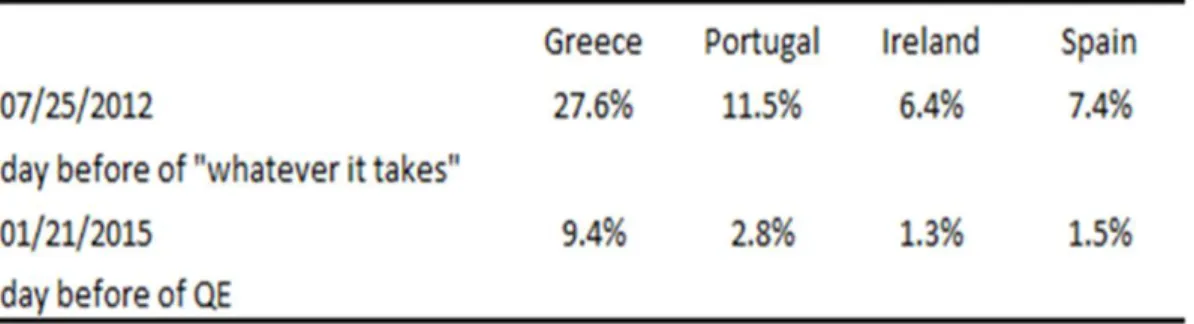
Participants in the sovereign bond market reacted strongly to the words of the president of the ECB. In fact, the “whatever it takes” gave rise to a long cycle of falling interest rates. Table 2 illustrates the huge decline in rates from the eve of the speech to the day which preceded the announcement of the formal QE, on January 22, 2015. Those movements might be interpreted as reflecting the expectation that a QE program might be implemented at some point down the road. At no point in the above mentioned time interval did Draghi discourage that line of reasoning.
As the interest rates on sovereign bonds followed its downward trend, the ECB continued to lower the monetary policy rate, a process which had been interrupted by two rate hikes in the first semester of 2011. That rate fell until it reached 0.05% (the lower bound) on September 4, 2014.
Further monetary accommodation was provided in the form of asset purchase. On September 4, 2014, the ECB announced a program to buy asset-back securities and covered bonds. The strategy acquired a new dimension with the expansion of the program (announced on January 22, 2015) to include bonds issued by euro area central governments, agencies and European institutions. The objective was to fulfil the “price stability mandate” and the plan was to make combined monthly purchases
Graph 5: GDP and Inflation in the Eurozone (%)
31
Applied Economics Research | Center for Monetary StudiesYear 3 | Number 5 | March. 2015
Table 2: Decline in 10-Year Government Bond Rates in Selected Eurozone Economies After Draghi´s “Whatever it Takes”
Source: Bloomberg.
in the amount of €60 billion and to stick to the program until “at least September 2016”.
Concluding remarks
Slow growth and deflationary forces are concerns related to the recent economic performance of the developed world. According to the IMF, the average annual rate of economic growth of the advanced economies was 1.5% in the last four years. This compares very unfavorably with 2.4% per annum, which is the historical average rate of expansion of that part of the world (1980 through 2014). The comparison is even more unfavorable if we recall that prior to the GFC, that is, from 1980 through 2007, that average rate was 2.8%. In the emerging market and developing economies, the annual rate of economic growth has acquired a declining tendency, from 7.4% in 2010 to an estimated 4.3% this year, but the average performance in the last four years (5.2%) was better than the historical performance of that group of countries (4.6% in 1980-2014).
Important authors of the past had taught us that macroeconomic stability and particularly good expectations about the future may give rise to too optimistic sentiments capable of leading to situations of excess debt and leverage and to the formation of bubbles. As the bubbles inevitably burst, financial crises and long recessions normally ensue.
32
Applied Economics Research | Center for Monetary StudiesYear 3 | Number 5 | March. 2015
The Great Recession seems to constitute one more illustration of this line of reasoning. Debt overhang, however, does not seem to be the only factor behind the poor performance of the advanced world in the post-crisis years. Apparently, the asymmetric way of correcting balance of payments disequilibria in the Eurozone (fiscal austerity in deficit countries and no adjustment in the main surplus economy) and real wages running considerably behind productivity gains in the developed countries have also contributed to that poor performance.
The secular stagnation hypothesis – examined more carefully at an earlier opportunity - is certainly another possible explanation. Such a hypothesis has to do with the idea that important structural changes (increased saving and a diminished demand for investments) had possibly occurred in the industrial world, probably starting before the GFC. As a result, aggregate demand contracted and the equilibrium real rate of interest (globally determined) fell, compelling central bankers to lower their policy rates, until they reached the zero lower bound. Possible reasons for those changes would be: a) a worsening of the income distribution causing an increased propensity to save; b) a diminished demand for capital goods due to slower population growth; c) modern industries are less capital intensive than old ones; d) a fall in the relative price of business equipment, implying less borrowing and spending.
Our intention in this essay has not been to exhaust the list of possible demand-related factors capable of explaining the sluggish economic growth of the developed world in the post-GFC years. The fact is that, independently from the relative importance of each factor, and in spite of policy interest rates at zero or close to it, aggregate demand is weak and inflation is very low, sometimes negative, depending on the measure we choose to look at. Wholesale and import prices experience negative rates of growth in important corners of the world. At the consumer level, they are either low, as in the US, or close to zero, as in the Eurozone.
Judging by the observed low levels of long-term interest rates, economic agents expect the present scenario to persist for quite some time. In the US, the care with which Fomc members are dealing with the issue of normalization of monetary policy seems to reflect lack of confidence on the resumption of the growth process on more solid terms –fear of acting prematurely is clearly present.
33
Applied Economics Research | Center for Monetary StudiesYear 3 | Number 5 | March. 2015
In Japan and the Eurozone, the main policy response to the prevailing environment has been quantitative easing, a strategy which does not seem to address the main obstacles to a more solid economic recovery. In parts of the Eurozone, deleveraging is either in its very beginning or did not get started yet, implying absence of borrowers for the liquidity injected into the banking system by the ECB. In Japan, the private sector shows no enthusiasm for resuming the borrowing activity, probably because entrepreneurs are having a hard time finding attractive investment opportunities, a problem which Japan may have in common with other mature economies and which cannot be fixed by means of quantitative easing.
In sum, there is no sign that the tensions associated with slow growth and deflationary pressures will disappear in the foreseeable future.