A MEMETIC ALGORITHM FOR LOGISTICS
NETWORK DESIGN PROBLEMS
by
Cristiano Baptista Faria Maciel
Submitted to the Department of Mathematics and Statistics
for the degree of
Master of Economic and Corporate Decision-Making
at the
LISBON SCHOOL OF ECONOMICS & MANAGEMENT
October 2014
Cristiano Maciel
A MEMETIC ALGORITHM FOR LOGISTICS NETWORK
DESIGN PROBLEMS
by
Cristiano Baptista Faria Maciel
Submitted to the Department of Mathematics and Statistics on October 15, 2014, in partial fulfillment of the
requirements for the degree of
Master of Economic and Corporate Decision-Making
Abstract
This thesis describes a memetic algorithm applied to the design of a three-echelon
logistics network over multiple periods with transportation mode selection and
out-sourcing. The memetic algorithm can be applied to an existing supply chain in order
to obtain an optimized configuration or, if required, it can be used to define a new
logistics network. In addition, production can be outsourced and direct shipments of
products to customer zones are possible. In this problem, the capacity of an existing
or new facility can be expanded over the time horizon. In this case, the facility cannot
be closed. Existing facilities, once closed, cannot be reopened. New facilities cannot
be closed, once opened. The heuristic is able to determine the number and locations
of facilities (i.e. plants and warehouses), capacity levels as well as the flow of products
throughout the supply chain.
KEYWORDS: Memetic Algorithm, Genetic Algorithm, Outsourcing.
Cristiano Maciel
Acknowledgments
To Prof. Teresa Melo, that was always available to help and guide me during this
process. Without her support, comments and suggestions this work would not be
possible to finish.
To the Saarland University of Applied Sciences that provided unique conditions to
work and live during this period at Saarbrücken, Germany.
To my family and friends that despite the distance, constantly give me support and
motivation to accomplish my purposes.
To everyone, a grateful thanks.
Contents
1 Introduction 8
2 Literature review 12
3 Mathematical formulation 18
3.1 Input data and decision variables . . . 18
3.2 Network redesign constraints . . . 22
3.3 Objective function . . . 28
3.4 Model enhancements . . . 29
4 Memetic Algorithm 31 4.1 Genetic algorithm . . . 32
4.1.1 Initial Population . . . 33
4.1.2 Genetic operators . . . 35
4.2 Local search . . . 40
Cristiano Maciel
5.2 Performance behaviour of different requirements of outsourcing(𝛽)and
direct shipments to clients (𝜆) . . . 46
5.2.1 Suggestions for improvements . . . 54
6 Conclusion 56
References 58
List of Figures
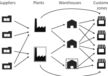
1-1 Possible configuration of a multi-echelon logistics network. . . 9
5-1 LND Model - Heuristic and Cplex performance . . . 46
5-2 LRD Model - Heuristic and Cplex performance . . . 46
5-3 LND Model - Value performance, |𝑇|= 4 . . . 47
5-4 LND Model - CPU Time performance, |𝑇|= 4 . . . 49
5-5 LRD Model - Value performance, |𝑇|= 4 . . . 50
5-6 LRD Model - CPU Time performance, |𝑇|= 4 . . . 51
5-7 LND Model - Value performance, |𝑇|= 6 . . . 51
5-8 LND Model - CPU Time performance, |𝑇|= 6 . . . 52
5-9 LRD Model - Value performance, |𝑇|= 6 . . . 53
Cristiano Maciel
List of Tables
2.1 Classification of the existing literature . . . 17
3.1 Index sets. . . 19
3.2 Fixed and variable costs. . . 20
3.3 Additional input parameters. . . 22
3.4 Decision variables. . . 23
5.1 Size of the test instances . . . 44
5.2 Cplex performance . . . 44
Chapter 1
Introduction
Logistics network design (LND) is a strategic planning process that aims to provide an
exceptional performance in order to achieve shareholder goals and clients satisfaction.
As result, LND is dedicated to process optimization by taking the following decisions:
∙ Defining the optimal number and location of facilities (e.g., manufacturing
plants and warehouses)
∙ Allocating capacity and technology requirements to facilities
∙ Deciding on the flow of products throughout the supply chain
In order to be competitive a company may consider redesigning its supply chain or
designing a new chain, depending on the company business requirements and
strat-egy objectives. If a company decides to enter a new market or to expand its product
segments, then designing a new logistics network (LND) is the most advantageous
decision. In contrast, if there is change in the market and business conditions, in
Cristiano Maciel
to adopt a restructuration of its supply chain through logistics network re-design
(LRD). Strategic network decisions have a direct influence on the competitiveness
of a company and it is crucial for management to have a framework for successful
tactical and operational supply chain processes. As highlighted by Ballou [4] and
Harrison [14], a network re-design project can result in a 5 to 15 percent reduction
of the overall logistics costs, with 10 percent being often achieved. In this thesis, an
Plants Warehouses Customer zones Suppliers
Figure 1-1: Possible configuration of a multi-echelon logistics network.
integrated and comprehensive view of the supply chain is taken by considering
sup-pliers, manufacturing facilities, warehouses, transportation channels, and customer
zones as shown in Figure 1-1. In an LRD approach, a network is already in place
with a number of plants and warehouses being operated at fixed locations (these
are the facilities marked by the dashed lines in the figure). A variety of decisions
have to be made regarding facility location and logistics functions along the supply
chain, such as opening new plants and/or warehouses at potential sites (the facilities
without dashed lines in Figure 1-1) and selecting their capacity levels from a set of
available discrete sizes. This is motivated by the fact that capacity is often purchased
in the form of equipment which is only available at a few discrete sizes. As strategic
planning for multiple time periods is considered, capacity can be acquired more than
once over the time horizon in the same location. Existing plants and warehouses
can be closed throughout the planning horizon. Alternatively, their capacities can
be expanded if a company forecasts future expansion into new markets or to meet
increasing product demand in current markets. In an LND approach, the scope of
the location decisions is limited to deciding on the optimal size, number, and
loca-tion of new facilities. Logistics decisions, the second group of key business decisions,
involve supplier selection in conjunction with procurement as well as production and
distribution decisions. Furthermore, a strategic choice between in-house
manufac-turing, outsourcing or a mixed approach is to be taken. In the network depicted
in Figure 1-1, multiple types of products are manufactured at plants by processing
sub-assemblies and components, hereafter called raw materials. The latter can be
procured from various suppliers taking into account their availability and cost.
Fin-ished products can be delivered to warehouses or shipped directly to customer zones.
The flow of goods throughout the network and the use of transportation modes are to
be determined in each time period. In addition, end products can also be purchased
from external sources and consolidated at the warehouses. The objective is to
deter-mine the optimal network configuration over a planning horizon so as to minimize
the total cost. The remainder of this thesis is organized as follows. In chapter 2, we
review the relevant literature dedicated to LND/LRD and describe its relation to our
Cristiano Maciel
for logistics network design and re-design. In chapter 4, the memetic algorithm is
described. In chapter 5, the heuristic performance is analyzed for a set of randomly
generated instances. Moreover, possible ways of improving the heuristic performance
are presented. In chapter 6, the main conclusions are exposed and recommendations
for future research are provided.
Chapter 2
Literature review
Beginning with the work of Geoffrion and Graves [12] on multi-commodity
distribu-tion network design in 1974, a large number of optimizadistribu-tion-based approaches have
been proposed for the design of logistics networks as shown by the recent surveys
of Melo et al. [17] and Mula et al. [22]. These works have resulted in significant
improvements in the modeling of these problems as well as in algorithmic and
com-putational efficiency. One of the reasons that contributes to such a large number of
literature references is the variety of characteristics that can be taken into account
in LND problems: type of planning horizon (single or multi-period), facility location
and sizing, number of echelons and distribution levels, multi-stage production taking
the bill of materials (BOM) into account, and transportation mode selection, among
others.
Although the timing of facility locations and expansions over an extended time horizon
is of major importance to decision-makers in strategic network design, the majority
Cristiano Maciel
et al. [7], Elhedhli and Goffin [10], Eskigun et al. [11], Olivares et al. [23], and Sadjady
and Davoudpour [24]. Our research is different in that a multi-period planning horizon
is considered. Unlike our work, in some multi-period LND problems facility sizing
is static, meaning that facilities cannot have their capacities expanded or contracted
over the planning horizon. The model proposed by Gourdin and Klopfenstein [13]
falls into this category.
We will focus next on multi-period LND and LRD problems with dynamic facility
sizing decisions. In particular, we will discuss the extent to which the features of the
model to be detailed in Section 3 differ from those reported so far in the literature.
To re-design a two-layer network, Antunes and Peeters [1] suggest a modeling
frame-work that allows opening new facilities and closing existing locations, as well as
reducing and expanding capacity. Budget constraints are taken into account over the
time horizon. To find the minimum discounted cost solution, the authors propose a
simulated annealing approach.
Melo et al. [16] study the re-design of a multi-echelon network considering facility
expansion and contraction. This feature is modeled through relocating capacity from
existing facilities to new facilities over the planning horizon. Network re-design
de-cisions (opening, closing, and relocating facilities) are subject to budget constraints
in each time period. General purpose optimization software is used to solve small
and medium-sized problem instances. Melo et al. [18, 19] also developed heuristic
procedures for this special form of network re-design. The numerical experiments
in-dicate that good solutions can be obtained for large-sized instances within acceptable
computational time.
Hinojosa et al. [15] address a multi-echelon, multi-commodity network re-design
prob-lem with inventory strategic decisions at warehouses and outsourcing of demand.
Commodities flow from manufacturing plants to customers via warehouses.
Out-sourced commodities are delivered directly to customers. An initial network
con-figuration is considered that gradually changes over a multi-period horizon through
opening new facilities and closing existing facilities. A lower bound is imposed on the
number of plants and warehouses operating in the first and last time periods. The
problem is solved using a Lagrangean-based procedure through decomposition into
simpler subproblems. A heuristic method is then applied to obtain a feasible solution.
Thanh et al. [25] consider a multi-period, multi-product logistics network comprising
suppliers, plants, warehouses (public and private), and customers. Strategic decisions
include facility location and capacity acquisition as well as supplier selection,
produc-tion, distribuproduc-tion, and inventory planning. In particular, plants and warehouses can
have their capacities expanded (but not contracted) over the time horizon.
Pro-duction decisions take into account the BOM and intermediate components can be
sub-contracted to an external plant. Furthermore, products flow downstream not
only between adjacent supply chain layers but also directly from plants to customers.
In addition, plants may exchange components. To identify the least-cost network
configuration, Thanh et al. [27] propose an LP-rounding heuristic. This method is
later improved by combining it with DC programming (cf. Thanh et al. [26]).
Bashiri and Badri [5] address the problem of designing a new supply chain network
with a similar topology to that considered in [25]. The objective is to find the network
Cristiano Maciel
time period. In this work, demand requirements may not be completely satisfied.
Strategic decisions include opening and expanding new plants and private
(company-owned) warehouses. In addition, public warehouses can be hired for a pre-specified
number of time periods and variable costs are charged for their operation. The
pro-posed model is extended in Bashiri et al. [6] through introducing different time scales
for strategic and tactical decisions. In particular, the latter are made in each time
period, whereas network design decisions are only made over a subset of periods of the
planning horizon. The models presented in [5, 6] are solved with a general-purpose
optimization solver. Later, Badri et al. [3] develop a Lagrangean-based approach.
Feasible solutions are obtained by dualising the budget constraints for opening new
facilities or expanding the capacities of existing facilities and adding some constraints
to the subproblems to guarantee feasibility.
Dias et al. [9] proposed a memetic algorithm for an LND problem involving opening,
closing, and re-opening facilities over a planning horizon with multiple periods.
Vari-ous mechanisms were employed to search the solution space. In addition,the decision
taken is able to set the search area and establish limits to the objective function.
In order to relate the existing literature to the LND and LRD problems that are
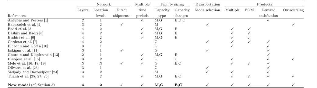
studied in this paper, a classification of the aforementioned works is given in Table 2.1.
This table is not intended to provide an exhaustive list of the features described in
this section but rather to illustrate the extent to which our research generalizes the
existing literature.
The characteristics of the surveyed LND and LRD problems are classified according to
five categories. The category “Network” comprises the number of layers in the supply
chain, including the customer level (column 2) and the number of layers involving
location decisions (column 3). Furthermore, it is specified whether products can be
distributed directly from higher level facilities to customer locations (column 4). The
second category (column 5) refers to the type of planning horizon. The category
“Facility sizing” summarizes the type of capacity decisions that can be made. To this
end, column 6 indicates if the size of each facility is limited (G: global capacities)
and if capacity levels are selected from a set of available discrete sizes (M: modular
capacities). In column 7, the type of capacity planning is given: expansion (E) and/or
downsizing (D) over the time horizon. Moreover, to distinguish network design from
network re-design problems, the latter are highlighted with the letter C, meaning
that existing facilities can be closed. The category in column 8 refers to the selection
of transportation modes. Finally, the category “Products” outlines characteristics
related to the number of products (column 9), multi-stage production taking into
account the BOM (column 10), satisfaction of demand requirements (column 11),
and the possibility of outsourcing components or end products as an alternative to
in-house manufacturing (column 11).
The last row of Table 2.1 highlights the main features of the model to be detailed
in Section 3. It can be seen that in our model various features are considered
si-multaneously in a multi-period planning context. To the best of our knowledge, this
integration of practically relevant features into a single model has not been addressed
Cristiano
Maciel
Network Multiple Facility sizing Transportation Products
Layers Location Direct time Capacity Capacity Mode selection Multiple BOM Demand Outsourcing References levels shipments periods type changes satisfaction
Antunes and Peeters [1] 2 1 X M,G E,D,C X
Babazadeh et al. [2] 3 2 X M X X
Badri et al. [3] 4 2 X M,G E X X
Bashiri and Badri [5] 4 2 X M,G E X X
Bashiri et al. [6] 4 2 X M,G E X X
Cordeau et al. [7] 4 2 G X X X X
Elhedhli and Goffin [10] 3 1 G X X
Eskigun et al. [11] 3 1 X G X X
Gourdin and Klopfenstein [13] 2 1 X M,G E X
Hinojosa et al. [15] 3 2 X G C X X X
Melo et al. [16, 18, 19] N N X X G E,C X X X
Olivares et al. [23] 3 1 G X X
Sadjady and Davoudpour [24] 3 2 M X X X
Thanh et al. [25, 27, 26] 4 2 X M,G E,C X X X X
New model (cf. Section 3) 4 2 X X M,G E,C X X X X X
C: Closing existing facilities
D: Downsizing (capacity contraction) E: Capacity expansion
G: Global capacities M: Modular capacities
N: No limit on the number of network layers and location levels
Table 2.1: Classification of the existing literature
Chapter 3
Mathematical formulation
In this section, we introduce a mathematical model for a comprehensive LRD problem.
The formulation integrates location and capacity choices for plants and warehouses
with supplier and transportation mode selection as well as outsourcing options over
multiple time periods. As will be seen, the model also can be used for designing a
new logistics network.
3.1 Input data and decision variables
Table 3.1 describes the index sets that are used, while Table 3.2 summarizes all costs.
For notational convenience, we introduce the set 𝑂𝐷 with all origin-destination pairs
in the logistics network (recall Figure 1-1):
Cristiano Maciel
The links (𝑠, ℓ) are used to transport raw materials 𝑟 ∈ 𝑅, while all other
origin-destination pairs concern links to move end products,𝑝∈𝑃.
Set Description
𝑇 Time periods
𝑆 Suppliers
𝐿𝑒 Existing plants at the beginning of the time horizon
𝐿𝑛 Potential sites for locating new plants
𝐿=𝐿𝑒∪𝐿𝑛 All plant locations
𝐾𝐿 Discrete capacity sizes that can be installed in plant locations
𝑊𝑒 Existing warehouses at the beginning of the time horizon
𝑊𝑛 Potential sites for locating new warehouses
𝑊 =𝑊𝑒∪𝑊𝑛 All warehouse locations
𝐾𝑊 Discrete capacity sizes that can be installed in warehouse
lo-cations
𝐶 Customer zones
𝑅 Raw materials
𝑃 End products
𝑀 Transportation modes
𝑂𝐷 All origin-destination pairs in the logistics network
Table 3.1: Index sets.
The parameters𝐹 𝐶𝑡,𝑗 and 𝑆𝐶𝑡,𝑗 reflect fixed costs associated with location decisions. The first term comprises the fixed costs of setting up an infrastructure for a new plant
or warehouse (e.g., property acquisition) in time period 𝑡. Facility closing costs (the
second term) are incurred when an existing plant or warehouse is closed in period 𝑡.
Other facility costs concern the acquisition of capacity in both new and existing
locations and the operation of that capacity. To this end,𝐼𝐶𝑡,𝑗,𝑘 =𝐼𝑡,𝑗,𝑘+
∑︀|𝑇|
𝜏=𝑡𝑂𝐶 𝑛 𝜏,𝑗,𝑘,
where 𝐼𝑡,𝑗,𝑘 denotes the fixed installation cost of capacity level 𝑘 ∈ 𝐾𝐿 ∪ 𝐾𝑊 in location 𝑗 ∈ 𝐿 ∪𝑊 in period 𝑡 ∈ 𝑇, and 𝑂𝐶𝑛
𝜏,𝑗,𝑘 is the fixed operating cost in
period 𝜏 ≥𝑡. The fixed costs 𝐼𝐶𝑡,𝑗,𝑘 reflect economies of scale. Expansion plans may result in extending the capacity of existing facilities and/or establishing new facilities
with given capacity.
Symbol Description
𝐹 𝐶𝑡,𝑗 Fixed cost of establishing a new facility in location 𝑗 ∈𝐿𝑛∪𝑊𝑛 in period 𝑡∈𝑇
𝑆𝐶𝑡,𝑗 Fixed cost of closing an existing facility in location 𝑗 ∈𝐿𝑒∪𝑊𝑒 in period 𝑡∈𝑇
𝐼𝐶𝑡,𝑗,𝑘 Cost of installing capacity level𝑘 ∈𝐾𝐿∪𝐾𝑊 in location 𝑗 ∈𝐿∪𝑊 in period 𝑡 ∈𝑇
𝑂𝐶𝑡,𝑗 Fixed cost of operating existing facility𝑗 ∈𝐿𝑒∪𝑊𝑒in period 𝑡∈𝑇
𝑃 𝐶𝑡,𝑠,𝑟 Cost of procuring one unit of raw material 𝑟 ∈ 𝑅 from supplier
𝑠 ∈𝑆 in period 𝑡 ∈𝑇
𝑀 𝐶𝑡,ℓ,𝑝 Cost of manufacturing one unit of product 𝑝∈𝑃 at plantℓ∈𝐿 in period 𝑡∈𝑇
𝑇 𝐶𝑡,𝑜,𝑑,𝑖,𝑚 Cost of shipping of one unit of item𝑖∈𝑅∪𝑃 using transportation mode𝑚∈𝑀 from origin𝑜 ∈𝑆∪𝐿∪𝑊 to destination𝑑∈𝐿∪𝑊∪𝐶
in period 𝑡 ∈𝑇
𝐸𝐶𝑡,𝑤,𝑝 Cost of purchasing one unit of product 𝑝 ∈ 𝑃 from an external source by warehouse 𝑤∈𝑊 in period 𝑡∈𝑇
Table 3.2: Fixed and variable costs.
Logistics costs include procurement, production, outsourcing, and distribution costs.
The latter depend on the choice of the transportation modes for moving raw materials
and end products through the network. The available transportation modes differ
with respect to their variable costs and capacities. For example, railroad and road
freight transport may be viable options with known trade-offs (cost, service time,
environmental impact). External costs concern the purchase of end products from
other business firms. The consolidation of outsourced products takes place at the
warehouses. A pre-specified percentage of the total customer demand for each end
product sets an upper bound on the total quantity that can be acquired from an
external source. This option may be attractive when the cost of setting up a new
Cristiano Maciel
Table 3.3 introduces additional input parameters. We assume that the available
capacity levels are sorted in non-decreasing order of their sizes. For plant locations
ℓ ∈ 𝐿 this means that 𝑄ℓ,1 < 𝑄ℓ,2 < . . . < 𝑄ℓ,|𝐾L|. Similar conditions hold for warehouse locations. As distinct technologies may be used by different plants to
manufacture a given product𝑝∈𝑃, we consider a production consumption factor𝜇ℓ,𝑝 for every plant location ℓ ∈ 𝐿. Moreover, the quantity of raw materials required to
manufacture one unit of a specific product may also differ among the various plants.
Plant-dependent BOMs are specified by the parameters 𝑎ℓ,𝑟,𝑝. In contrast, the usage
of warehouse capacity by an end product does not depend on the warehouse location,
thus a consumption factor 𝛾𝑝 is assumed for every 𝑝∈𝑃.
Constant 𝛼𝑗 is used to specify a minimum throughput level at facility 𝑗, the latter being defined by multiplying 𝛼𝑗 by the capacity installed in location 𝑗 ∈ 𝐿∪𝑊. In this way, it will be guaranteed that facilities are operated at least at a meaningful
level.
All decisions are implemented at the beginning of each time period. As indicated in
Table 3.4, strategic decisions on facility location and capacity acquisition are ruled
by binary variables, while tactical logistics decisions are described by continuous
variables. The statuses of new facilities (i.e. plants, warehouses) over the time horizon
are controlled by the variables𝑦𝑡,𝑗𝑛 . If a new plant or warehouse is established at the beginning of period𝑡in site𝑗 ∈𝐿𝑛∪𝑊𝑛then𝑦𝑛
𝑡,𝑗 = 1and𝑦𝑛𝜏,𝑗 = 0for all other periods
𝜏 ∈𝑇, 𝜏 ̸=𝑡. Regarding the existing facilities, if facility𝑗 ∈𝐿𝑒∪𝑊𝑒 ceases to operate at the beginning of period 𝑡 then 𝑦𝑡,𝑗𝑒 = 1 and 𝑦𝜏,𝑗𝑒 = 0 for all periods 𝜏 ∈ 𝑇, 𝜏 ̸= 𝑡. Observe that if a new facility𝑗 is available in period 𝑡 then ∑︀𝑡
𝜏=1𝑦 𝑛
Symbol Description
𝑎ℓ,𝑟,𝑝 Number of units of raw material 𝑟 ∈ 𝑅 required to manufacture one unit of product 𝑝∈𝑃 in plant ℓ∈𝐿
𝑄𝑆𝑡,𝑠,𝑟 Capacity of supplier 𝑠∈𝑆 for raw material𝑟 ∈𝑅 in period 𝑡 ∈𝑇
𝜇ℓ,𝑝 Production capacity usage by one unit of product 𝑝 ∈ 𝑃 in plant
ℓ ∈𝐿
𝛾𝑝 Handling capacity usage by one unit of product 𝑝 ∈ 𝑃 in a
ware-house
𝑄𝑒
𝑗 Capacity of existing facility 𝑗 ∈𝐿𝑒∪𝑊𝑒 available at the beginning of the time horizon
𝑄𝑗,𝑘 Capacity of level 𝑘 ∈ 𝐾𝐿 ∪𝐾𝑊 that can be installed in facility
𝑗 ∈𝐿∪𝑊
𝑄𝑗 Maximum overall capacity of facility𝑗 ∈𝐿∪𝑊 in each time period 𝑄𝑀𝑡,𝑜,𝑑,𝑚 Capacity of transportation mode𝑚∈𝑀 from origin𝑜 ∈𝑆∪𝐿∪𝑊
to destination 𝑑∈𝐿∪𝑊 ∪𝐶 in period 𝑡 ∈𝑇
𝜎𝑖,𝑚 Capacity utilization factor by one unit of item 𝑖∈ 𝑅∪𝑃 in trans-portation mode 𝑚 ∈𝑀
𝑑𝑡,𝑐,𝑝 Demand of customer zone 𝑐∈𝐶 for product𝑝∈𝑃 in period 𝑡∈𝑇
𝜆𝑡,𝑝 Fraction of the total demand for product𝑝∈𝑃 in period𝑡∈𝑇 that can be delivered directly from plants to customers; 0≤𝜆𝑡,𝑝 <1
𝛽𝑡,𝑝 Fraction of the total demand for product 𝑝 ∈ 𝑃 in period 𝑡 ∈ 𝑇 that can
be supplied by an external source; 0≤𝛽𝑡,𝑝 <1
𝛼𝑗 Number between zero and one for a facility 𝑗 ∈ 𝐿∪𝑊 (to set a
minimum
throughput level at the facility)
Table 3.3: Additional input parameters.
if an existing facility 𝑗 is operated in period𝑡 then ∑︀𝑡
𝜏=1𝑦 𝑒 𝜏,𝑗 = 0.
3.2 Network redesign constraints
In this section, we describe in detail the specific constraints that compose our LRD
Cristiano Maciel
Symbol Description
𝑦𝑛
𝑡,𝑗 1 if a new facility is established in location 𝑗 ∈𝐿𝑛∪𝑊𝑛 in period
𝑡 ∈𝑇, 0 otherwise 𝑦𝑒
𝑡,𝑗 1 if an existing facility in location 𝑗 ∈ 𝐿𝑒 ∪𝑊𝑒 is closed at the beginning of period 𝑡 ∈𝑇, 0 otherwise
𝑢𝑡,𝑗,𝑘 1 if capacity level 𝑘 ∈𝐾𝐿∪𝐾𝑊 is installed in location 𝑗 ∈ 𝐿∪𝑊 in period 𝑡 ∈𝑇, 0 otherwise
𝑥𝑡,𝑜,𝑑,𝑖,𝑚 Quantity of item 𝑖 ∈ 𝑅∪𝑃 shipped in period 𝑡 ∈ 𝑇 from origin 𝑜 to destination 𝑑,(𝑜, 𝑑)∈𝑂𝐷, using transportation mode 𝑚∈𝑀 𝑧𝑡,𝑤,𝑝 Quantity of product 𝑝∈𝑃 provided by an external source to
ware-house 𝑤∈𝑊 in period 𝑡∈𝑇
Table 3.4: Decision variables.
Supplier-related constraints
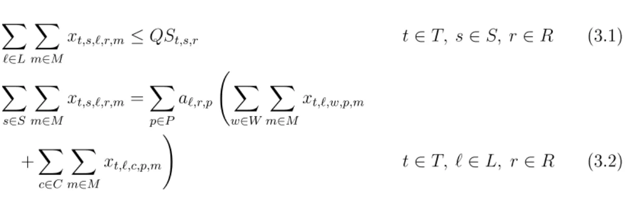
Supplier selection and procurement of raw materials are ruled by the following
con-ditions:
∑︁
ℓ∈𝐿
∑︁
𝑚∈𝑀
𝑥𝑡,𝑠,ℓ,𝑟,𝑚 ≤𝑄𝑆𝑡,𝑠,𝑟 𝑡 ∈𝑇, 𝑠∈𝑆, 𝑟∈𝑅 (3.1)
∑︁
𝑠∈𝑆
∑︁
𝑚∈𝑀
𝑥𝑡,𝑠,ℓ,𝑟,𝑚 =
∑︁ 𝑝∈𝑃 𝑎ℓ,𝑟,𝑝 (︃ ∑︁ 𝑤∈𝑊 ∑︁ 𝑚∈𝑀 𝑥𝑡,ℓ,𝑤,𝑝,𝑚 +∑︁ 𝑐∈𝐶 ∑︁ 𝑚∈𝑀 𝑥𝑡,ℓ,𝑐,𝑝,𝑚 )︃
𝑡 ∈𝑇, ℓ∈𝐿, 𝑟 ∈𝑅 (3.2)
Constraints (3.1) limit the quantity of each raw material provided by a supplier.
Equalities (3.2) ensure that the total amount of raw material𝑟 purchased by a plant
is used to manufacture end products. Observe that the expression within brackets
on the right-hand side defines the total quantity of product 𝑝 manufactured in time
period 𝑡 in plant ℓ. End products can be distributed to warehouses or delivered
directly to customer zones.
Facility location and capacity acquisition constraints
The following constraints impose the required conditions for setting up new facilities
and closing existing facilities over the planning horizon. In addition, they also rule the
installation of capacity and its expansion. For notational convenience, let us denote
𝐾𝑗 =𝐾𝐿 if 𝑗 ∈𝐿and 𝐾𝑗 =𝐾𝑊 if 𝑗 ∈𝑊.
∑︁
𝑡∈𝑇
𝑦𝑡,𝑗𝑛 ≤1 𝑗 ∈𝐿𝑛 ∪ 𝑊𝑛 (3.3)
𝑦𝑡,𝑗𝑛 ≤ ∑︁
𝑘∈𝐾j
𝑢𝑡,𝑗,𝑘 ≤ 𝑡
∑︁
𝜏=1
𝑦𝑛𝜏,𝑗 𝑡 ∈𝑇, 𝑗∈𝐿𝑛 ∪ 𝑊𝑛
(3.4)
∑︁
𝑘∈𝐾j
𝑢𝑡,𝑗,𝑘 ≤1− |𝑇|
∑︁
𝜏=1
𝑦𝜏,𝑗𝑒 𝑡 ∈𝑇, 𝑗∈𝐿𝑒 ∪ 𝑊𝑒
(3.5) ∑︁ 𝑘∈𝐾j 𝑄𝑗,𝑘 ∑︁ 𝑡∈𝑇
𝑢𝑡,𝑗,𝑘 ≤𝑄𝑗
∑︁
𝑡∈𝑇
𝑦𝑡,𝑗𝑛 𝑗 ∈𝐿𝑛 ∪ 𝑊𝑛 (3.6)
𝑄𝑒𝑗
(︃
1−∑︁
𝑡∈𝑇
𝑦𝑒𝑡,𝑗
)︃ + ∑︁ 𝑘∈𝐾j 𝑄𝑗,𝑘 ∑︁ 𝑡∈𝑇
𝑢𝑡,𝑗,𝑘 ≤𝑄𝑗
(︃
1−∑︁
𝑡∈𝑇
𝑦𝑡,𝑗𝑒
)︃
𝑗 ∈𝐿𝑒 ∪ 𝑊𝑒 (3.7)
Constraints (3.3) impose that at most one new facility (plant/warehouse) can be
established in a potential location over the time horizon. Moreover, once open, new
facilities cannot be closed. Constraints (3.4), resp. (3.5), rule the installation of
capacity in new, resp. existing, locations. In each time period, at most one capacity
level can be selected provided that a facility is already operating in that site. On the
other hand, if a new facility is established in a given period then a capacity level must
Cristiano Maciel
existing facility has its capacity extended then it cannot be closed. Since the location
variables 𝑦𝑒
𝑡,𝑗 are binary, the term
∑︀|𝑇|
𝜏=1𝑦 𝑒
𝜏,𝑗, which appears on the right-hand side of
(3.5), takes a non-negative integer value. If this term is zero then facility𝑗 ∈𝐿𝑒∪𝑊𝑒
remains in operation over the whole time horizon. As a result, the right-hand side
of (3.5) is equal to one, thereby setting an upper bound on the number of capacity
expansions that are permitted in each period. If ∑︀|𝑇|
𝜏=1𝑦 𝑒
𝜏,𝑗 = 1 then facility 𝑗 was closed in some period 𝜏 and so the right-hand side of (3.5) becomes zero. In this
case, the facility cannot be expanded in any period (recall that the variables 𝑢𝑡,𝑗,𝑘 that appear on the left-hand side of (3.5) are binary). Finally, notice that values of
∑︀|𝑇|
𝜏=1𝑦 𝑒
𝜏,𝑗 larger than one are not possible as this would yield a negative right-hand
side of (3.5). These constraints would become invalid since 𝑢𝑡,𝑗,𝑘 represent binary variables.
Constraints (3.6), resp. (3.7), set a limit on the capacity expansion of each new, resp.
existing, plant or warehouse.
Constraints related to capacity utilization
The next sets of constraints establish minimum and maximum capacity utilization
limits on both plants and warehouses. These limits depend on the acquisition of
ca-pacity over time. In every location, the caca-pacity available in each period is determined
by 𝐴𝑛 𝑡,𝑗 = ∑︀ 𝑘∈𝐾j 𝑄𝑗,𝑘 𝑡 ∑︀ 𝜏=1
𝑢𝜏,𝑗,𝑘 𝑡 ∈𝑇, 𝑗∈𝐿𝑛 ∪ 𝑊𝑛
𝐴𝑒
𝑡,𝑗 = 𝑄𝑒𝑗
(︂ 1− 𝑡 ∑︀ 𝜏=1 𝑦𝑒 𝜏,𝑗 )︂ + ∑︀ 𝑘∈𝐾j 𝑄𝑗,𝑘 𝑡 ∑︀ 𝜏=1
The above capacities are used for processing end products at plants and warehouses.
For ease of exposition, we introduce two expressions for the total quantity processed
by plants and warehouses:
𝐹𝐿 𝑡,𝑗 = ∑︀ 𝑝∈𝑃 𝜇𝑗,𝑝 (︂ ∑︀ 𝑤∈𝑊 ∑︀ 𝑚∈𝑀
𝑥𝑡,𝑗,𝑤,𝑝,𝑚 +
∑︀ 𝑐∈𝐶 ∑︀ 𝑚∈𝑀 𝑥𝑡,𝑗,𝑐,𝑝,𝑚 )︂
𝑡∈𝑇, 𝑗 ∈𝐿 𝐹𝑊 𝑡,𝑗 = ∑︀ 𝑝∈𝑃 𝛾𝑝 ∑︀ 𝑐∈𝐶 ∑︀ 𝑚∈𝑀
𝑥𝑡,𝑗,𝑐,𝑝,𝑚 𝑡∈𝑇, 𝑗 ∈𝑊
Constraints (3.8) and (3.9) guarantee that the total quantity of products
manufac-tured by each plant must be within pre-defined lower and upper limits in each time
period. Constraints (3.10)–(3.11) impose similar conditions on warehouses. Observe
that the lower capacity utilization limits refer to minimum throughputs corresponding
to a given percentage of the maximum capacities.
𝛼𝑗𝐴𝑛𝑡,𝑗 ≤𝐹 𝐿 𝑡,𝑗 ≤𝐴
𝑛
𝑡,𝑗 𝑡∈𝑇, 𝑗 ∈𝐿
𝑛 (3.8)
𝛼𝑗𝐴𝑒𝑡,𝑗 ≤𝐹 𝐿 𝑡,𝑗 ≤𝐴
𝑒
𝑡,𝑗 𝑡∈𝑇, 𝑗 ∈𝐿
𝑒 (3.9)
𝛼𝑗𝐴𝑛𝑡,𝑗 ≤𝐹𝑡,𝑗𝑊 ≤𝐴𝑛𝑡,𝑗 𝑡∈𝑇, 𝑗 ∈𝑊𝑛 (3.10)
𝛼𝑗𝐴𝑒𝑡,𝑗 ≤𝐹 𝑊 𝑡,𝑗 ≤𝐴
𝑒
𝑡,𝑗 𝑡∈𝑇, 𝑗 ∈𝑊
Cristiano Maciel
Transportation, outsourcing, and demand-related constraints
∑︁
𝑖∈𝑅∪𝑃
𝜎𝑖,𝑚𝑥𝑡,𝑜,𝑑,𝑖,𝑚≤𝑄𝑀𝑡,𝑜,𝑑,𝑚 𝑡∈𝑇, (𝑜, 𝑑)∈𝑂𝐷, 𝑚∈𝑀 (3.12)
∑︁ ℓ∈𝐿 ∑︁ 𝑐∈𝐶 ∑︁ 𝑚∈𝑀
𝑥𝑡,ℓ,𝑐,𝑝,𝑚 ≤𝜆𝑡,𝑝
∑︁
𝑐∈𝐶
𝑑𝑡,𝑐,𝑝 𝑡∈𝑇, 𝑝 ∈𝑃 (3.13)
∑︁
𝑐∈𝐶
∑︁
𝑚∈𝑀
𝑥𝑡,𝑤,𝑐,𝑝,𝑚 =
∑︁
ℓ∈𝐿
∑︁
𝑚∈𝑀
𝑥𝑡,ℓ,𝑤,𝑝,𝑚+𝑧𝑡,𝑤,𝑝 𝑡∈𝑇, 𝑤 ∈𝑊, 𝑝∈𝑃 (3.14)
∑︁
𝑤∈𝑊
𝑧𝑡,𝑤,𝑝 ≤𝛽𝑡,𝑝
∑︁
𝑐∈𝐶
𝑑𝑡,𝑐,𝑝 𝑡∈𝑇, 𝑝 ∈𝑃 (3.15)
∑︁
ℓ∈𝐿
∑︁
𝑚∈𝑀
𝑥𝑡,ℓ,𝑐,𝑝,𝑚 +
∑︁
𝑤∈𝑊
∑︁
𝑚∈𝑀
𝑥𝑡,𝑤,𝑐,𝑝,𝑚 = 𝑑𝑡,𝑐,𝑝 𝑡∈𝑇, 𝑐∈𝐶, 𝑝∈𝑃 (3.16)
Capacity constraints on individual transportation modes are imposed by (3.12). For
supplier-plant links (𝑠, ℓ), these constraints rule the utilization of transportation
ca-pacity for raw materials 𝑟 ∈ 𝑅, while for all other origin-destination pairs
equali-ties (3.12) involve end products. Inequaliequali-ties (3.13) limit the quantity of direct
de-liveries from plants to customers for every product. Constraints (3.14) guarantee the
conservation of product flows for all operated warehouses in each time period. These
constraints along with inequalities (3.10) and (3.11) state that outsourced products
also use the handling capacity available at warehouses. Constraints (3.15) impose
an upper limit on the total outsourced quantity per product type. Finally,
con-straints (3.16) ensure the satisfaction of all customer demands over the time horizon.
Domains of variables
The following constraints (3.17)-(3.21) represent non-negativity and binary
condi-tions.
𝑥𝑡,𝑜,𝑑,𝑖,𝑚 ≥ 0 𝑡 ∈𝑇, (𝑜, 𝑑)∈𝑂𝐷, 𝑖∈𝑅∪𝑃, 𝑚∈𝑀 (3.17)
𝑧𝑡,𝑤,𝑝 ≥ 0 𝑡 ∈𝑇, 𝑤∈𝑊, 𝑝∈𝑃 (3.18)
𝑦𝑡,𝑗𝑛 ∈ {0,1} 𝑡 ∈𝑇, 𝑗∈𝐿𝑛∪𝑊𝑛 (3.19)
𝑦𝑡,𝑗𝑒 ∈ {0,1} 𝑡 ∈𝑇, 𝑗∈𝐿𝑒∪𝑊𝑒 (3.20)
𝑢𝑡,𝑗,𝑘 ∈ {0,1} 𝑡 ∈𝑇, 𝑗∈𝐿∪𝑊, 𝑘 ∈𝐾𝐿∪𝐾𝑊 (3.21)
3.3 Objective function
The objective function (3.22) minimizes the overall strategic and logistics costs. Fixed
deter-Cristiano Maciel
mined by the remaining terms.
Min ∑︁
𝑡∈𝑇
∑︁
𝑗∈𝐿n∪𝑊n
𝐹 𝐶𝑡,𝑗𝑦𝑡,𝑗𝑛 +
∑︁
𝑡∈𝑇
∑︁
𝑗∈𝐿e∪𝑊e
𝑆𝐶𝑡,𝑗𝑦𝑒𝑡,𝑗 +
∑︁ 𝑡∈𝑇 ∑︁ 𝑗∈𝐿∪𝑊 ∑︁ 𝑘∈𝐾j
𝐼𝐶𝑡,𝑗,𝑘𝑢𝑡,𝑗,𝑘+
∑︁
𝑡∈𝑇
∑︁
𝑗∈𝐿e∪𝑊e
𝑂𝐶𝑡,𝑗 (︃ 1− 𝑡 ∑︁ 𝜏=1
𝑦𝜏,𝑗𝑒
)︃ + ∑︁ 𝑡∈𝑇 ∑︁ 𝑤∈𝑊 ∑︁ 𝑝∈𝑃
𝐸𝐶𝑡,𝑤,𝑝𝑧𝑡,𝑤,𝑝+
∑︁ 𝑡∈𝑇 ∑︁ 𝑠∈𝑆 ∑︁ ℓ∈𝐿 ∑︁ 𝑟∈𝑅 ∑︁ 𝑚∈𝑀
(𝑃 𝐶𝑡,𝑠,𝑟 +𝑇 𝐶𝑡,𝑠,ℓ,𝑟,𝑚) 𝑥𝑡,𝑠,ℓ,𝑟,𝑚+
∑︁ 𝑡∈𝑇 ∑︁ ℓ∈𝐿 ∑︁ 𝑗∈𝑊∪𝐶 ∑︁ 𝑝∈𝑃 ∑︁ 𝑚∈𝑀
(𝑀 𝐶𝑡,ℓ,𝑝+𝑇 𝐶𝑡,ℓ,𝑗,𝑝,𝑚) 𝑥𝑡,ℓ,𝑗,𝑝,𝑚+
∑︁ 𝑡∈𝑇 ∑︁ 𝑤∈𝑊 ∑︁ 𝑐∈𝐶 ∑︁ 𝑝∈𝑃 ∑︁ 𝑚∈𝑀
𝑇 𝐶𝑡,𝑤,𝑐,𝑝,𝑚𝑥𝑡,𝑤,𝑐,𝑝,𝑚 (3.22)
The problem of re-designing an existing logistics network is modeled by the objective
function (3.22) subject to the constraints (3.1)–(3.21). We remark that for 𝐿𝑒 = ∅ and 𝑊𝑒 =∅, the formulation reduces to the special case of designing a new network.
3.4 Model enhancements
There are various ways of enhancing the LRD model. A simple strategy is to
mul-tiply the right-hand side of the capacity constraints (3.12) by appropriate sets of
facility location variables. For the flow of end products from plants and warehouses
to customer zones, this corresponds to replacing inequalities (3.12) by
∑︁
𝑝∈𝑃
𝜎𝑝,𝑚𝑥𝑡,𝑗,𝑐,𝑝,𝑚 ≤𝑄𝑀𝑡,𝑗,𝑐,𝑚 𝑡
∑︁
𝜏=1
𝑦𝑛𝜏,𝑗 𝑡∈𝑇, 𝑗 ∈𝐿𝑛∪𝑊𝑛, 𝑐∈𝐶, 𝑚∈𝑀
(12a)
∑︁
𝑝∈𝑃
𝜎𝑝,𝑚𝑥𝑡,𝑗,𝑐,𝑝,𝑚 ≤𝑄𝑀𝑡,𝑗,𝑐,𝑚
(︃ 1−
𝑡
∑︁
𝜏=1
𝑦𝑒𝜏,𝑗
)︃
𝑡∈𝑇, 𝑗 ∈𝐿𝑒∪𝑊𝑒, 𝑐∈𝐶, 𝑚∈𝑀
(12b)
Similar transformations can be easily performed for transportation modes linking
suppliers to plants. In this case, raw materials cannot be moved from supplier 𝑠 to
plantℓ with transportation mode𝑚 in time period𝑡unless plantℓis operated in that
period. For plant-warehouse pairs, transportation modes cannot be selected unless
the origin plant and the destination warehouse are both operated. In this case, it
is necessary to duplicate inequalities (3.12) for these types of transportation links,
thereby adding |𝑇| · |𝐿| · |𝑊| · |𝑀| new constraints to the LRD model. We opted
to transform inequalities (3.12) without increasing the model size. To this end, for
plant-warehouse pairs we extend the right-hand side of (3.12) to ensure that products
Cristiano Maciel
Chapter 4
Memetic Algorithm
A memetic algorithm (MA) is an evolutionary algorithm that makes use of a local
search heuristic. The general idea behind an MA is to combine the advantages of
evolutionary operators that identify interesting regions of the search space, with local
neighbourhood search that quickly finds good solutions in a small region of the search
space.
The primary objective of the developed MA is to set the status and size of facilities
(the values of the binary decision variables) in order to obtain feasible solutions to
LND/LRD problems. In this algorithm, a solution/an individual is composed by a
set of closed and open facilities. The MA includes the following procedures:
1. Create initial population - P(0)
2. Apply local search to P(0)
3. Binary tournament selection
4. Crossover
5. Facility status correction procedure
6. Mutation
7. Capacity correction procedure
8. Apply local search to new population
Two criteria are used to stop the MA procedure. One is by setting a maximum
number of generations. Thereby, when the MA achieves the established number
of generations the procedure terminates. The other criterion defines a maximum
number of generations without improvement of the best solution. Currently, the
MA procedure stops if there is not an improvement of the best solution over 60% of
generations.
4.1 Genetic algorithm
In this work, the genetic representation is set up of two chromosomes, the S-chromosome
that represents the statuses of the facilities (i.e. open/closed) in every period and the
F-chromosome that describes the capacity sizes available at the active facilities. The
number of chromosomes in each solution is equal to the number of time periods while
the number of genes in each chromosome is equal to the number of existing and new
facilities. However, in the F-chromosome, each gene has three alleles referring to three
different capacity levels k (𝑘 ∈𝐾𝐿∪𝐾𝑊).
For each given choice of the binary variables (S and F-chromosomes), the original
Cristiano Maciel
the flow of products and the outsourcing quantities). Each sub-problem is solved to
optimality with Cplex. Its objective function value represents the solution fitness.
4.1.1 Initial Population
The initial population procedure aims at creating a set of solutions that will be used
by the algorithm to generate new individuals in the next generations. In order to
create feasible solutions, the following features are considered:
∙ The total capacity available in time period t (at plants and warehouses) must
cover the demand requirements in that period(𝑡 ∈𝑇).
∙ In every time period t, the capacity installed in each facility j (𝑗 ∈ 𝐿∪𝑊)
cannot exceed the global capacity limit of that facility.
Although these two features are crucial to ensure the feasibility of a solution, they do
not guarantee the quality of the solution with respect to the objective function value.
Naturally, the random selection of facilities to be operated does not ensure that the
best set of facilities is selected to satisfy the demand. In fact, the initial solutions are
typically "expensive" as they represent logistics networks with more capacity than
the one needed to cover the demand. In order to readjust the choice of capacity sizes,
a local search procedure is applied. Often, this technique helps to improve the quality
of the initial solutions.
The initial population, P(0), is initialized with four solutions, independently of the
number of time periods or customer zones. Preliminary numerical tests indicated that
this seems to be a good choice. Observe that initializing P(0) with more individuals
will have a strong impact on the time performance of the algorithm. On the other
hand, taking less individuals will have a negative effect on the population
diversifica-tion.
After each new generation, the new individuals are added to the previous population,
originating the new population.
Generation of the initial population:
1. For each period[t], (𝑡∈𝑇)
1.1 Determine the minimum demand requirements to be satisfied by plants
and warehouses in period[t] (𝑡∈𝑇)
1.2 Separately for existing plants and warehouses (𝑗 ∈ 𝐿𝑒 ∪ 𝑊𝑒), evaluate available capacity in period[t]
1.2.1 If available capacity is not enough to satisfy the demand in period[t]
then randomly select a facility[j] (𝑗 ∈𝐿∪𝑊)
1.2.2 Determine installed capacity at selected facility j until period 𝑡−1
1.2.3 Select the most suitable size k (𝑘 ∈ 𝐾𝐿 ∪ 𝐾𝑊), starting with the smallest size
2. Apply local search (Section 4.2, p. 40)
Cristiano Maciel
4.1.2 Genetic operators
Binary tournament selection
From the pool of N individuals (with N denoting the number of existing parents), N-1
individuals will be selected by applying a binary tournament. This is equivalent to
selecting the N-1 best individuals of the pool, but in this procedure, the randomness
of the two solutions selected to participate in the binary tournament defines the
sequence of parents that will be used in the crossover. For example, combining the
winner of the binary tournament [i] with the winner of the binary tournament [i+1]
(𝑖+ 1≤𝑁−1)will yield one pair of parents for crossover. Hence, in the next genetic
operator, the pairs of parents are already established.
Crossover
This genetic operator will act through two random crossover points, OX𝑗, j ∈ {1,2},
as proposed by Michalewicz and Fogel [20]. Thus, three arguments will be created that
will influence the generation of the offsprings. The three arguments are as follows:
∙ [1;𝑂𝑋1]
∙ ]𝑂𝑋1;𝑂𝑋2]
∙ ]𝑂𝑋2;|𝑇|]
The offspring [i] will be created by combining the genes of the S-chromosome and
F-chromosome of the two parents. This offspring will receive new genes from the
parent [𝑖+ 1] by changing the 1st and 3rd arguments given above and keeping the
original genes from the 2nd argument belonging to parent [i].
The number of crossovers (q) depends on the number of parents available, however
the total number of parents can be an even or odd number. As a result, if the total
number of parents is odd, the parent[q] will not have a pair to generate a son. To
prevent this situation, the following formula is used:
⌊𝑞⌋=
⌊︂Number of parents in current generation −0.5 2
⌋︂
For example, if the number of available parents is 5, the crossover procedure can only
be applied twice. In the first one, the procedure will be applied to parent[1] and
parent[2] and in the second time to parent[3] and parent[4].
Crossover procedure:
1. Select randomly crossover points OX𝑗,j ∈ {1,2}
2. Select two parents, parent[i] and parent [i+1], 𝑖∈ {1, ..., 𝑞}
2.1 From[1, 𝑂𝑋1], transfer the genes of the S-chromosome and F-chromosome: 2.1.1 parent[i] to son[i+1]
2.1.2 parent[i+1] to son[i]
2.2 From]𝑂𝑋1, 𝑂𝑋2], transfer the genes of the S-chromosome and F-chromosome: 2.2.1 parent[i] to son[i]
2.2.2 parent[i+1] to son[i+1]
Cristiano Maciel
2.3.1 parent[i] to son[i+1]
2.3.2 parent[i+1] to son[i]
3. Call "Facility status correction" procedure
At this stage, it is required to take into account the possibility that a facility is
assigned an invalid status. For example, if in the 2nd argument some facilities have
installed capacity, then it is necessary to verify if those facilities are open. If this is
not the case then a status correction procedure is applied.
Facility status correction procedure:
1. For each solution[i] (𝑖∈𝑁), determine in the S-chromosome the open period[t] (𝑡∈𝑇)of each facility[j] (𝑗 ∈𝐿∪𝑊)
1.1 If gene[t][j] of facility[j] = 1: S-chromosome[𝜏] : for period[𝜏] (𝜏 ∈ {𝑡+ 1, ...,|𝑇|}), set genes [𝜏][𝑗] = 0
2. For each solution[i](𝑖∈𝑁), analyze the installed capacity size k(𝑘 ∈𝐾𝐿∪𝐾𝑊), in period[t] (𝑡 ∈𝑇) for each facility[j] (𝑗 ∈𝐿∪𝑊)
2.1 If facility size[t][j][k] = 1, update installed capacity[t][j].
2.2 If installed capacity[t][j] > Global capacity of facility[j]
2.2.1 F-chromosome: from period [𝜏](𝜏 ∈ {𝑡, ...,|𝑇|}), set genes[𝜏][𝑗][𝑘] = 0
2.2.2 S-chromosome: set genes [𝜏][𝑗] = 0
Mutation
Mutation is an operator that allows the diversification of the population and is applied
to offsprings generated by the crossover procedure. However, not all elements benefit
from this operator. With a mutation probability (Pm), as indicated by Mühlenbein et
al. [21],𝑃 𝑚 = 1.7
𝑁×|𝑇|, the mutation probability decreases in each new generation due
to adding new individuals to the population. As a result, mutation is more likely to be
used in early generations and only when a random number(random mutation∈[0,1])
is less than Pm.
This procedure is applied to facilities by selecting randomly one active facility (current
facility) and another that is not operated yet (new facility). After selection, the genes
of the S-chromosome and F-chromosome are swapped from the current facility to the
new selected facility.
Mutation procedure:
1. Calculate Pm
2. Select son[i] for mutation
3. Generate a random continuous number, random nutation (random mutation∈ [0,1]), to decide if mutation is applied to current son[i]. If random mutation <
Pm, go to 4. Otherwise, mutation is not applied.
4. Select randomly two genes[j], 𝑗 ∈ 𝐿∪𝑊
Cristiano Maciel
5. Swap S-chromosome and F-chromosome
6. Call "Facility capacity correction" procedure
7. Select son[i+1] and go to 3
After this procedure, it is required to take into account the transferred capacity into
the new facility, because the global capacities are different from facility to facility
and may transform a feasible solution into an infeasible one. To prevent this from
happening, a capacity correction procedure is applied after mutation. This procedure
analyzes the installed capacity of a facility during its active time periods and verifies
if the global capacity limit is satisfied.
In case of an infeasible solution, the capacity correction procedure will restrict the
installed capacity of the facility and in addition, a new facility will be opened to
satisfy the demand[t] that otherwise could not be covered.
Facility capacity correction procedure:
1. For each open facility[j] (𝑗 ∈ 𝐿∪𝑊) analyze the already installed size k (𝑘 ∈
𝐾𝐿∪𝐾𝑊), in period[t] (𝑡∈𝑇). Set k = current size
2. For each period, analyse if Installed capacity[t] < Total demand[t] and facility
size[t][j][k] = 1
2.1 For each facility[t][j], regarding the global capacity of facility[j], select the
most suitable size k, defined as new size k (current size<new size≤𝑘).
2.2 If installed capacity[t] with new size ≤Global capacity of facility[j]
2.2.1 S-chromosome: update the period in which the facility is opened
2.2.2 F-chromosome: for facility[j] in period t, set current size = 0 and new
size = 1
3. If Installed capacity[t] < Total demand[t], it is required to open a new facility
3.1 Select randomly a new non-active facility
3.2 Starting with k = 1 (current size), select the most appropriate size (new
size) for facility[j], as follows
3.2.1 If facility size[t][j][k] ≤ Global capacity of facility[j], then
3.2.2 S-chromosome: if required, update the period in which the facility is
opened
3.2.3 F-chromosome: set current size = 0 and new size = 1
4. If Installed capacity[t] < Total demand[t], return to step 3
4.2 Local search
This procedure tries to improve the fitness of new individuals. To start this
proce-dure two facilities belonging to the same network layer are randomly selected. The
first corresponds to an active facility (current facility) and the second one to a
non-operated facility (new facility). In order to keep diversity, a facility (new facility) can
only be selected once.
After a new facility has been selected, the genes of the S-chromosome and the
F-chromosome are swapped. At this stage, due to the different characteristics of the
Cristiano Maciel
As a result of these differences, four possibilities can occur by changing the current
size of the new facility:
∙ The current size installed at facility[j] at period[t] cannot supply demand and
a larger size must be selected.
∙ The current size can supply demand and the global capacity is satisfied. As a
result, no changes are required.
∙ Due to the different capacity sizes of the new facility it is possible to select a
smaller size.
∙ The solution has an excess of capacity and it is possible not to use the selected
facility. This may occur when at previous local searches, the surplus of installed
capacity is much higher than the required to satisfy demand.
In the current procedure, the term "most feasible new size" is introduced and it means
that the selected size is the best option because it does not compromise the global
capacity of the facility[j] and also allows the satisfaction of demand[t].
With this procedure, 15% of the neighbours available in the solution are visited. A
higher percentage of neighbors visited will lead to an increase of the computational
time required to solve the problem and a lower percentage will have a residual impact
on the diversification of the solutions. Preliminary tests indicated that 15% is an
appropriate value for this parameter. The total number of neighbours of a solution is
equal to the number of existing and new facilities. For example, if a solution contains
two existing facilities and 10 new facilities, the number of local searches will be equal
to⌈(2 + 10)×0.15⌉= 2.
The purpose of this procedure is to find a facility that is able to satisfy demand[t],
but it is less expensive than the "initial facility". However, if there is enough installed
capacity to supply demand[t] without the initial/new facility, this facility is removed
from the solution.
Local search procedure:
1. Select initial facility: randomly choose a facility that is operated (𝑗 ∈𝐿∪𝑊)
2. Select new facility: randomly choose a non-operated facility[j’]
3. Swap the genes of the S-chromosome and F-chromosome from the initial facility
to the new facility
3.1 Determine the current size k (𝑘 ∈𝐾𝐿∪𝐾𝑊) installed
3.2 Select the most feasible new size k or if possible remove current facility[j]
4. If current size̸=new size, evaluate solution using Cplex to solve the subproblem
and keep new solution, independently if it improves or not.
5. If current size = new size, apply local search to a 2nd neighbourhood
5.1 To another "new" facility, apply steps 1, 2 and 3
5.2 If new solution has enough capacity to satisfy demand[t](𝑡∈𝑇), the global
capacity of facility[j] is satisfied and the new solution value is better than
the previous one, keep the new solution. Else, restore initial solution.
Cristiano Maciel
Chapter 5
Computational results
In total, 60 test instances were randomly generated with different time periods and
different number of customers (50, 75, and 100). Half of the instances belong to
the network redesign (LRD) class and the other half to the network design (LND)
class. The interested reader is referred to Cortinhal et al. [8] for further details. Six
different combinations of the parameters 𝜆𝑡,𝑝 = 𝜆 and 𝛽𝑡,𝑝 = 𝛽 were considered as follows: 𝜆𝑡,𝑝 ∈ {0%,10%},𝛽𝑡,𝑝 ∈ {0%,10%,20%}for every𝑡∈𝑇,𝑝∈𝑃, thus yielding in total 360 cases. For each parameter combination, a CPU time limit of 8h was set
for IBM ILOG Cplex 12.6.0. Both the model and the heuristic were implemented in
C++. All experiments were performed on a PC with a 3.5 GHz Intel Core i7-3770K
processor, 8 GB RAM and running Windows 7 (64-bit). The heuristic was run with
5 generations. This parameter results from results from running the test instances
with different values for the maximum number of generations. A number larger than
5 leads to an increase of the computational time required to create all generations. In
contrast, lower quality solutions could be obtained when the number of generations
is less than 5. Moreover, the heuristic also stops when there is not an improvement
of the best solution over 60% of the generations.
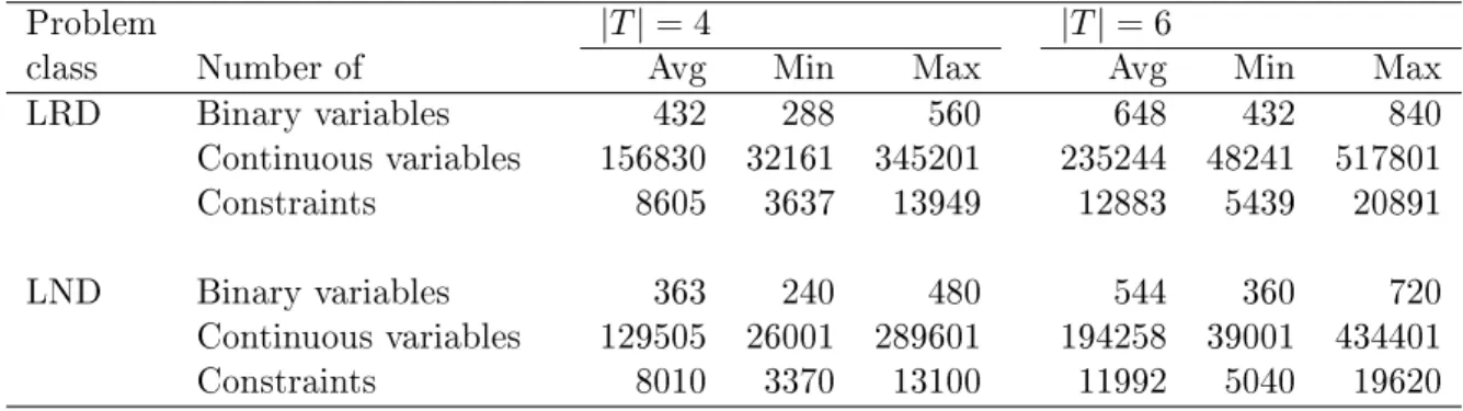
In the next table the sizes of the test instances are presented for both problem variants
and |𝑇| ∈ {4,6}. The table gives the average, minimum and maximum number of
binary and continuous variables and the number of constraints. Table 5.2 displays a
Problem |T|= 4 |T|= 6
class Number of Avg Min Max Avg Min Max
LRD Binary variables 432 288 560 648 432 840
Continuous variables 156830 32161 345201 235244 48241 517801
Constraints 8605 3637 13949 12883 5439 20891
LND Binary variables 363 240 480 544 360 720
Continuous variables 129505 26001 289601 194258 39001 434401
Constraints 8010 3370 13100 11992 5040 19620
Table 5.1: Size of the test instances
classification of the best solutions found by Cplex within the pre-specified time of 8h
is given.
Cplex Network
solutions LND model LRD model
|T|= 4 Optimal 64.44% 74.44%
Non-Optimal 35.56% 25.56%
|T|= 6 Optimal 46.67% 67.78%
Non-Optimal 53.33% 32.22%
Table 5.2: Cplex performance
5.1 Memetic Algorithm versus Cplex
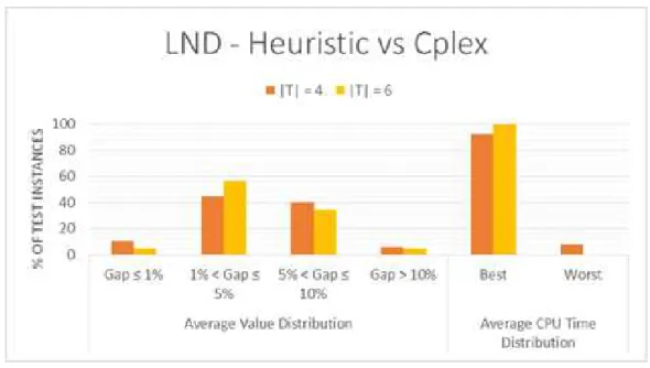
In Figures 5-1 and 5-2, the performance of the heuristic is compared to Cplex. In
iden-Cristiano Maciel
tified by the heuristic and Cplex are compared as follows:
𝐺𝑎𝑝= Heuristic performance−Cplex performance
Cplex performance
The analysis is focused on two parameters, the average objective value and the
aver-age CPU time. The first one is obtained by stratifying the gaps into five groups and
for each group the average value gap is calculated. A similar procedure is applied
to obtain the average gap time, but in this case the data is split into two groups,
the best time of the heuristic versus Cplex (Best) and worst time of heuristic versus
Cplex (Worst).
The analysis is conducted by comparing the LND problem class with the LRD
prob-lem class in order to allow an easier interpretation and comparison of each network
performance.
LND instances require the opening of more new facilities than LRD instances and as
a result, more facilities must be selected to satisfy demand. However, due to the
ab-sence of existing facilities in the LND problem class, the time required by the heuristic
to analyse capacity restrictions is smaller. Consequently, the CPU time performance
of the heuristic is better in the LND class than in the LRD class. However, it is harder
for the heuristic to find the better combination of individuals that will constitute a
solution in the LND instances. As a result, the objective value performance is better
in the LRD class.
Figure 5-1: LND Model - Heuristic and Cplex performance
Figure 5-2: LRD Model - Heuristic and Cplex performance
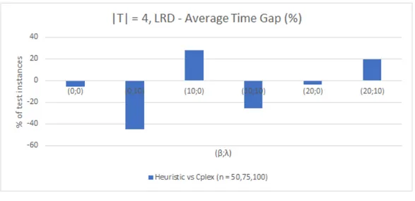
5.2 Performance behaviour of different requirements
of outsourcing
(𝛽
)
and direct shipments to clients
(𝜆)
Cristiano Maciel
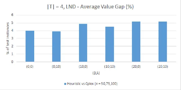
to the objective function value and the CPU time performance. Once a new logistics
network is built from the beginning (LND), the gap between the installed capacity
and the demand is under the influence of the selected facilities. This means, that
more efficient selections will lead to smaller gaps. By analysing Figure 5-3, we verify
that the smaller average gap is 3.91% for 𝛽 = 0% and 𝜆 = 10% (at most 10% of the
production is sent directly to customer zones). In contrast, the biggest average gap
is 5.17% for 𝛽 = 20% and 𝜆 = 10%. In this case, at most 20% of the demand is
outsourced and 10% of the manufactured products is sent directly to customer zones.
There is a significant decrease of capacity handled by plants but not by warehouses.
Due to the maximum outsourcing level (20%), less plants are required but the heuristic
is not sensitive to minimize the gap between the installed capacity and the required
capacity to supply demand. Typically, the installed capacity is much higher than the
required capacity, leading to expensive solutions. Figure 5-4 shows that a slightly
Figure 5-3: LND Model - Value performance, |𝑇|= 4
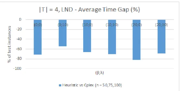
different behaviour is observed regarding the CPU time. This KPI (Key Performance
Indicator) has a better performance for instances with𝛽 ∈ {0%, 20%} and𝜆= 10%.
When at most 10% of the demand can be shipped directly from plants to customers,
less warehouse capacity is necessary and less time is consumed to select a warehouse
and a proper size to install. Hence, the time required by the heuristic to find a feasible
set of warehouses to satisfy the demand is smaller.
Analysing the transition from 𝛽 = {0%, 20%} and 𝜆 = 0% to 𝛽 = {0%, 20%} and 𝜆 = 10%, it is possible to observe a decrease of performance. Despite 10% of the
total demand being shipped directly to customer zones, once again the heuristic is
not able to select the most appropriate facilities in order to minimize the gap between
the installed capacity and the required capacity to supply demand. The exception is
the pair 𝛽 =𝜆 = 10%because the quantity sent by plants, without direct shippment
to customers, is equal to the quantity received by warehouses. In this scenario, at
most 10% of the plants’ production is outsourced and 10% of the demand is shipped
directly to customer zones. For 𝛽 = 10% and 𝜆 = 0%, the average time gap is
-65.56% comparatively to -70.18% for 𝛽 = 10% and 𝜆 = 10%. This particular case
has a performance similar to the case with 𝛽 =𝜆 = 0% (-71.26%). The performance
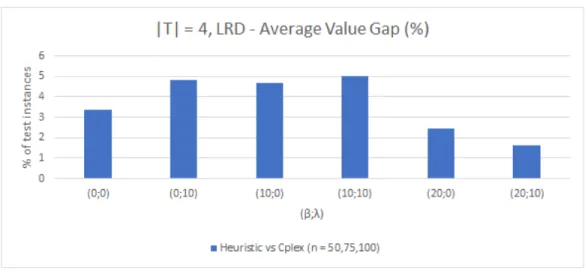
of the heuristic in the LRD class differs significantly from the LND class. In the
latter case, there is no installed capacity in the network at the beginning of the time
horizon. In contrast, in the LRD network, at the starting period there is already
installed capacity and often, less facilities must be opened to satisfy demand.
Comparing the test instances 𝛽 ∈ {0%, 10%} and 𝜆 = 0% with 𝛽 ∈ {0%, 10%}
and 𝜆 = 10%, normally it leads to an increase of the average gap, because with
Cristiano Maciel
Figure 5-4: LND Model - CPU Time performance, |𝑇|= 4
capacities must be adjusted in order to turn solution more efficient in terms of costs.
This production is shipped directly to customer zones, but the heuristic is not able
to select the most appropriate warehouses to supply demand. As a result, more
expensive solutions are created. This is the same reason as with the LRD network,
but because there is already installed capacity, less random selections must be done,
leading to smaller average value gaps compared to an LND network. In the LRD
test instances, the higher average value gap is 5.01% for 𝛽 = 10% and 𝜆 = 10%. In
contrast, the best average value gap is 1.63% for 𝛽 = 20% and 𝜆= 10%.
The heuristic performance greatly improves for𝛽 = 20%and 𝜆∈ {0%,10%}because
less quantity must be handled by plants, as at most 20% of the demand requirements
can be outsourced. Additionally, when 10% of the plants’ production is shipped
directly to customer zones, less facilities (warehouses) must be opened. In Figure
5-6 it is possible to analyse the average time gaps of LRD test instances for |T| =
4. For 𝛽 = {10%, 20%} and 𝜆 ∈ {0%, 10%} with exception of 𝛽 = 𝜆 = 10%,
Figure 5-5: LRD Model - Value performance, |𝑇|= 4
Cplex is able to obtain the optimal solution faster than the heuristic. In two cases
(𝛽 = {10%, 20%}), less quantity must be handled by plants and consequently, the
number of required plants is smaller. The same logic is valid when𝜆 = 10%, because
this implies that direct shipments to customer zones are possible. In the LRD test
instances, Cplex is able to take advantage of existing facilities to obtain less expensive
solutions. Hence, better solutions are generated by Cplex.
Next, Figures 5-7 to 5-10 are representative of the heuristic performance for |T| =
6 and both problem classes. It is possible to observe a significant difference of the
heuristic performance compared to the instances with |T| = 4.
In Figure 5-7, the average value gaps are slightly higher compared to |T| = 4. For |T|
= 6 and the LND test instances, the heuristic must select more facilities to supply
demand, and so more plants and warehouses must be opened. The heuristic is not
sensitive in order to minimize the gap between the total installed capacity in time
Cristiano Maciel
Figure 5-6: LRD Model - CPU Time performance, |𝑇|= 4
able to select appropriate facilities and this is once again the cause of these positive
gaps.
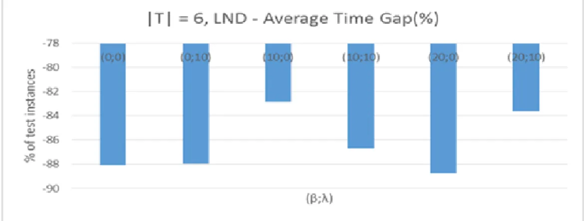
Regarding the CPU time performance for |T| = 6, there is a significant improvement
Figure 5-7: LND Model - Value performance, |𝑇|= 6
of the heuristic performance. In the "worst" case the heuristic was able to find a
solution in 82.83% of the instances (𝛽 = 10% and 𝜆 = 0%) faster than Cplex and
at the "better" this value increases to 88.73% (𝛽 = 20% and 𝜆 = 0%). With |T|
= 6, more data must be analysed and Cplex spends more time to identify feasible
solutions that are on average 4.63% (𝛽 = 10% and 𝜆 = 0%) and 5.91% (𝛽 = 20%
and 𝜆= 0%) cheaper than the heuristic solutions. Cplex takes more time to identify
a feasible solution. However, it is able to do a better selection of the facilities that
must operate, thus minimizing the total cost. In contrast, the heuristic is faster at
obtaining a feasible solution but the selection of the facilities that must be opened is
not as good as with Cplex. Hence, the heuristic solutions are more expensive.
Figure 5-8: LND Model - CPU Time performance, |𝑇|= 6
In Figures 5-9 and 5-10, the performance of the LRD class is presented for |T| = 6.
Again, there is a significant difference of the heuristic behaviour compared to |T| =
4. The average value gaps are higher, with a minimum gap of 3.74% (𝛽 = 10% and
𝜆= 0%) and a maximum gap of 5.73% (𝛽 = 20% and 𝜆= 10%).
In contrast to |T| = 4, with |T| = 6 the heuristic is able to perform better than Cplex
with respect to the average time gaps. In the "worst" case, the heuristic was 20.78%
Cristiano Maciel
Figure 5-9: LRD Model - Value performance, |𝑇|= 6
average 3.74% (𝛽 = 10% and 𝜆= 0%) more expensive. In the "better" performance
case, the heuristic identifies a feasible solution 63.27% (𝛽 = 0% and 𝜆 = 10%) faster
than Cplex with a cost that is 4.44% higher (on average). The heuristic is able to
Figure 5-10: LRD Model - CPU Time performance,|𝑇|= 6
find a feasible solution faster than Cplex. However, this comes at a cost with respect
to the quality of the solution obtained, which is lower than the one identified by