Abstract— In this research, fuzzy goal programming model for aggregate production and logistics planning with interval demand and uncertain production capacity is proposed. Two fuzzy goals are considered in the model; profit goal and change of workforce level goal. In conventional aggregate production planning (APP) models, logistics planning is not included. Even it is a critical criterion that creates extra cost. Moreover, demand is considered as crisp demand, which is not realistic. Actual demand is uncertain in nature and does not exactly equal to forecast demand. So, APP with interval demand that the best solution of possible demand can be selected is proposed in this research. Uncertain capacity is also considered in the proposed model. The proposed model can extremely increase profit and reduce change of workforce level. Furthermore, uncertain demand and production capacity are also cooperated, which make the model more realistic for the industrial applications. A case study of a real factory is illustrated to show the effectiveness of the proposed model.
Index Terms— Fuzzy goal, APP, interval demand, logistics planning
I. INTRODUCTION
GGREGATE production planning (APP) is concerned with matching supply and demand of forecasted and
varying customer orders over the medium term, often from 3 to 18 months in advance [1], [2]. An APP problem is about determining the maximize profit and minimize workforce, and inventory levels for each period of the planning horizon for a given set of production resources and constraints [3]. Generally, multiple objectives are considered such as maximize profit, minimize late orders, and minimize workforce level changes [3]. These objectives conflict in nature. Both deterministic and stochastic models have been proposed for modeling APP problems [4]-[6]. One of the most effective methods for solving multiple objectives problem is ―Goal Programming‖, (GP) [7]-[10]. However, considerable uncertainty was ignored. Stochastic models of APP can deal with uncertainty but they were hard to solve and statistical estimations proved inefficient because of
Manuscript received January 5, 2011; revised January 21, 2011. This work was supported in part by the Thailand Research Fund (TRF), the National Research Council of Thailand (NRCT), the Commission on Higher Education of Thailand and the Faculty of Engineering, Thammasat University, Thailand.
R. Yimmee is a graduate Student of Industrial Engineering, Industrial Engineering department, Faculty of Engineering, Thammasat University, Rangsit campus, Klongluang, Pathum-thani, 12120, Thailand. (corresponding author; e-mail: [email protected]).
B. Phruksaphanrat is an Assistance Professor, ISO-RU, Industrial Engineering department, Faculty of Engineering, Thammasat University, Rangsit campus, Klongluang, Pathum-thani, 12120, Thailand (e-mail: [email protected]).
lacking of statistical observation [11]. Heuristic approaches also have been presented [12]-[13]. However, problem constraints are not considered.
A suitable way to model imprecise data of APP problem is to use fuzzy set. Fuzzy set concept has been applied to APP in many literatures [14]-[16]. Many fuzzy goal programming (FGP) models were also proposed for solving multiple objective decision making problem with fuzzy environment [2], [17]-[21]. Most of them consider fuzzy goals, fuzzy capacity or fuzzy coefficients using conventional APP model [22]-[23], which logistics planning is not included. Moreover, uncertain demand may not exactly equal to forecast demand which is normally used as target level of demand for each period. Demand may deviate in a small range from this target value. If the appropriate level of demand, which suits for the actual capacity, can be selected from the possible interval then the appropriate production plan can be generated.
This paper considers a case study for APP application of a manufacturing company. This company produces plastic parts for automotive and electronic industries. It has some problems due to existing APP based on human experience and crisp information such as insufficient workforce level, shipment delay, excessive inventory level and unsatisfied demand. There are two issues to be concerned. Firstly, they feel uncomfortable to estimate the demand in each period as a constant using forecast demand. If they under-estimate the demand, an opportunity loss of sales and profit will occur. On the other hand, if they over-estimate the demand especially during peak demand periods, costly overtime, unnecessary subcontracting, and inventory holding will occur. Secondly, the company feels that the production output is not limited by the fixed capacity. In reality, the capacity can be deviated in a small range of a negative or a positive direction due to machine breakdown, adjustability or improvement of machine capacity. Moreover, conventional APP models do not concern about transportation cost. So, in this research the FGP model for aggregate production and logistics planning with interval demand and uncertain production capacity is proposed to solve the problem of this manufacturing company.
II. MODEL FORMULATION
A. Problem Description and Notations
APP model is developed to satisfy the case study problem. The company produces n types of products based on forecast demand in each planning horizon period (t): Two objective functions are considered in this case; to maximize profit and to minimize changes of workforce.
Fuzzy Goal Programming for Aggregate
Production and Logistics Planning
Ratiros Yimmee and Busaba Phruksaphanrat
Member, IAENG
1. Notations of parameters and variables 1.1 Indices:
i number of product types, i = 1,2,…,n. t number of periods in the planning horizon, t = 1,2,…,T.
1.2 Input parameters:
Pri selling price per unit of product type i, (Baht/unit).
CIi inventory carrying cost per unit of product i, (Baht/unit).
CBi backorder cost per unit of product i, (Baht/unit).
CPi production cost per unit of product i, (Baht/unit).
CSi subcontract cost per unit of product i, (Baht/unit).
CTi transportation cost per trip of product i, (Baht/trip).
COnt overtime cost per unit for normal working day in period t, (Baht/unit).
COh1t, COh2t overtime cost per unit for holiday during 8:00 am -5:00 pm and after 5:00 pm in period t, (Baht/unit).
CWt average salary per worker in period t, (Baht/worker).
CHt hiring and training cost per worker in period t, (Baht/worker).
CFt downsizing cost per worker in period t, (Baht/worker).
PHi production capacity rate of product i. (units/hour).
RHt maximum number of allowable regular hours per worker in period t, (hours/worker). Dit forecast demand of product i in period t, (units).
Smaxi, Bmaxi maximum subcontract and backorder quantities of product i, (units/month). Imax maximum inventory level in each period,
(units/month).
Wmaxi, Wmini maximum and minimum workforce level of product i in each period, (workers). PTmaxi maximum quantities of product i in each trip of transportation, (units/trip).
Onmaxt maximum number of allowable overtime hours per worker for normal working day in period t, (hours/worker).
Oh1maxt, Oh2maxt maximum number of allowable overtime hours per worker for holiday during 8:00 am - 5:00 pm and after 5:00 pm in period t, (hours/worker).
Imax maximum inventory level, (units).
Dmaxi, Dmini maximum and minimum quantities of forecast demand of product i in each period, (units).
Ii0, Bi0 initial number of inventory and backorder level of product i, (units).
W0 initial number of workers in period t, (workers).
1.3 Decision Variables:
dit forecast demand in an interval of product i in period t, (units).
Bit backorder quantities of product i in period t, (units).
Iit inventory level of product i in period t, (units).
Pit regular production of product i in period t, (units).
Oit overtime production of product i in period t, (units).
POnit overtime production for normal working day of product i in period t, (units).
POh1it, POh2it overtime production for holiday during 8:00 am - 5:00 pm and after 5:00 pm of product i in period t, (units).
Sit subcontracted production of product i in period t, (unit).
NTit number of trip for transportation normal delivery of product i in period t, (trips).
NTBit number of trip for transportation backorder delivery of product i in period t, (trips).
Wt regular production workers in period t, (workers).
Wit regular production workers of product i in period t, (workers).
WOit overtime workers of product i in period t, (workers).
WOnit overtime workers for normal working day of product i in period t, (workers).
WOh1it , WOh2it overtime workers for holiday during 8:00 am - 5:00 pm and after 5:00 pm of product i in period t, (workers).
Ht hired workers in period t, (workers). Ft fired workers in period t, (workers).
2. Objective functions
Two objective functions are considered in the proposed model.
2.1 Maximization of profit objective (z1): Profit comes from revenue of actual demands sent to customer minus costs of backordering, production, overtime, subcontracting, inventory and costs related to workforces. This objective is the main objective for all companies.
(1) 2.2 Minimization change of workforce levels (z2): Change of workforce level means the total numbers of hiring and firing in every period. This objective related to human resource management and morale of workers.
(2)
3. Constraints
period as shown in (3).
, . (3)
3.2 Production constraints: Production of regular time should not greater than production quantities generated by worker during regular time, which can be represented by (4). , (4)
3.3 Overtime constraints: Overtime for normal working day, overtime for holiday during 8:00 am -5:00 pm and after 5:00 pm for each product in each period are represented by (5)-(7), respectively. These overtime productions should not greater than overtime production quantities generated by overtime worker for each product in each period. Total overtime production in each period is summarized as shown in (8). , . (5)
, . (6)
, . (7)
, . (8)
3.4 Backorder and subcontract constraints: Backorder and subcontract quantities should not exceed the maximum allowable limit as shown in (9), (10). , . (9)
, . (10)
3.5 Inventory constraints: The inventory level cannot exceed the maximum allowable limit since there are limited warehouse spaces that can be shown as (11). , . (11)
3.6 Workforce constraints: Number of workers in each period is equal to the number of workers in previous period plus workers being hired at that period minus the number of workers being laid off at that period as shown in (12). Equation (13) shown that the total number of workers in period t is equal to the summation of the workers for all product. The number of worker for product i in period t should not less than the minimum number of workers and should not greater than the maximum number of workers of each product in each period as shown in (14). , . (12)
, . (13)
, . (14)
3.7 Overtime workforce constraints: The total number of overtime worker in normal working day for all products in every period should not less than the total number of regular workers of all products in every period as shown in (15). The total number of overtime worker in holiday during 8:00 am – 5:00 pm for all products in every period should not less than the total number of workers after 5:00 pm for all products in every period and should not greater than the number of workers in regular time of all products in every period as shown in (16). Overtime workers are able to transfer from workers of one product to another product. , (15)
, (16)
3.8 Transportation constraints: Number of trip for transportation normal delivery of product i in period t should not less than the demand of product i in period t divided by the maximum capacity for each trip of product i as shown in (17). Number of trip for transportation backorder delivery of product i in period t should also not less than backorder quantities of product i in period t divided by maximum capacity for each trip of product i as shown in (18). , . (17)
, . (18)
B. Fuzzy Goal Programming (FGP) Model with Interval Demand and Fuzzy Production Capacity Constraint. FGP normally uses to solve multiple objective decision making problems [15], [16]. In this research Preemptive Fuzzy Goal Programming (P-FGP) has been applied. Two fuzzy goals are concerned; profit and change of workforce level. P-FGP is suitable for this problem since the first goal (profit goal) is extremely important than the second goal (change of workforce level). Defining membership function of each goal is based on the Positive-Ideal Solution (PIS) and the Negative-Ideal Solution (NIS) [20]. The PIS is the best possible solution when each objective function is optimized. The NIS is the feasible and worst value of each objective function. Triangular membership function is considered as shown in Fig. 1 [15]-[16], [21]. Membership function can be written as (19). , (19) where, , k. (20)
, k. (21)
Profit goal ( ) and change of workforce level goal ( ) can be written as (22), (23).
(z )k
zk k
1
0
k k
k k k k
.
(22)
. (23)
In (22), dit is introduced for determination of demand within an interval of possible demand quantities for product i in period t that should not less than the minimum number of demands and should not greater than the maximum number of demands of each product in each period as shown in (24). Then, (3), (17) has been changed to (25), (26). , . (24)
, . (25)
, . (26)
Production capacity (PHi) is also considered as fuzzy capacity, ); . , represent optimistic, most-likely and pessimistic production capacity rate of product i, (units/hour). So, (4)-(7) can be rewritten as: , . (27)
, . (28)
, . (29)
, . (30)
P-FGP with interval demand and fuzzy production capacity can be shown as: Lexicographically maximize {1 ,2 }, (31)
subject to , k = 1, 2. (32)
, k = 1, 2. (33)
, k = 1, 2. (34)
, k = 1, 2. (35)
k = 1, 2. (36)
(9)-(16), (18), (24)-(30), where is the satisfaction level of the objective kth and is the desired level of satisfaction level of objective kth. Wang (1997) suggested converting using most-likely criterion. Then, . (37)
In the proposed method, three models can be generated based on optimistic, most-likely and pessimistic criteria because decision maker may need more information than just know only most-likely case. For most-likely criterion, Wang (1997)’s method is applied by substitute with (37). For optimistic and pessimistic criteria, and are used, respectively. So, three solutions are obtained from the P-FGP model for optimistic, most-likely and pessimistic criteria.
III. ACASE STUDY
A case study is presented to demonstrate the proposed model. The company under consideration is a plastic injection factory for automotive and electronic parts. The planning horizon is 6 months. There are 5 groups of products (A, B,…,E) by customers. Regular production is 8 hours per shift. Two shifts a day.
Average inventory cost per unit (CIi) is 0.0076 Baht. The maximum allowable inventory level in each period (Imax) is 100,000 units. The maximum allowable backorder level (Bmaxi) is twenty percentage of forecast demand.
Initial workforce level (W0) is 248 workers. Other information is given in the following tables.
TABLE I
THE BASIC DATAFOR EACH PRODUCT TYPE
Product A B C D E
Pri 47.00 0.85 30.00 20.00 8.00
CBi 9.40 0.17 6.00 4.00 1.60
CSi 39.38 0.00 34.26 0.00 0.00
CPi 19.42 0.49 15.66 5.92 1.62
CTi 1,200 0* 1,200 100 800
COni 8.31 0.25 2.74 1.03 0.48
COh1i 11.08 0.33 3.65 1.37 0.64
COh2i 16.62 0.50 5.48 2.06 0.96
PHi 6 140 8 30 80
Smaxi 50,000 0 100,000 0 0
Ii0 0 15,600 0 3,200 20,800
Bi0 28,000 0 66,000 0 0
Wmaxi 136 24 60 48 32
Wmini 68 12 30 24 16
PTmaxi 20,000 0 10,000 10,000 35,000
*Product B currently uses mill-run system so transportation cost is not concerned.
TABLE II
THE BASIC DATAIN EACH PERIOD
Period 1 2 3 4 5 6
CWt 5,600 5,400 5,200 5,800 5,800 6,000 CHt 4,560 3,800 3,990 4,560 4,560 4,180 CFt 16,800 16,200 15,600 17,400 17,400 18,000
RHt 384 320 336 384 384 352
Onmaxt 144 120 126 144 144 132
Oh1maxt 112 160 160 96 112 144
Oh2maxt 42 60 60 36 42 54
TABLE III
CRISP DEMAND DATAIN EACH PERIOD
Period DA DB DC DD DE
1 568,000 448,000 496,400 744,800 1,988,000
2 484,500 473,200 349,200 460,800 1,288,000 3 424,000 532,000 423,600 552,200 1,433,600
4 384,000 464,000 469,600 668,800 1,688,800 5 368,000 468,600 421,200 682,600 1,788,600
6 320,400 404,200 444,800 724,800 1,866,000
TABLE IV
INTERVAL DEMAND DATAIN EACH PRODUCT
Product A B C D E
TABLE V
PRODUCTION CAPACITY DATAIN EACH PRODUCT
Product A B C D E
PHi
-4 94 6 21 54
PHi +
8 187 11 40 107
TABLE VI
P-FGP WITH CRISP DEMANDSAT 1 = 0.8
Period BA BB BC BD BE
1 113,600 0 99,280 4,002 0
2 41,216 0 69,840 0 0
3 0 0 0 0 0
4 0 0 0 0 0
5 0 0 0 0 0
6 0 0 0 0 0
Period IA IB IC ID IE
1 0 0 0 0 0
2 0 0 0 0 0
3 0 0 0 0 0
4 0 0 0 0 0
5 0 0 0 0 0
6 0 0 0 0 0
Period SA SB SC SD SE
1 50,000 0 100,000 0 0
2 50,000 0 12,214 0 0
3 50,000 0 0 0 0
4 29,964 0 0 0 0
5 0 0 0 0 0
6 0 0 0 0 0
Period PA PB PC PD PE
1 313,344 432,400 92,160 473,321 983,040 2 261,120 473,200 76,800 394,434 819,200 3 274,176 532,000 80,640 414,156 860,160 4 313,344 464,000 92,160 473,321 983,040 5 313,344 468,600 92,160 473,321 983,040 6 287,232 404,200 84,480 433,878 901,120
Period OA OB OC OD OE
1 119,056 0 270,960 264,277 984,160 2 245,764 0 289,626 70,368 468,800 3 141,040 0 412,800 138,044 573,440 4 40,692 0 377,440 195,479 705,760 5 54,656 0 329,040 209,279 805,560 6 33,168 0 360,320 290,922 964,880
Period NTBNTA,
A
NTB, NTBB
NTC, NTBC
NTD, NTBD
NTE, NTBE
1 24, 6 - 35, 10 46, 1 37, 0
2 28, 2 - 50, 7 74, 0 57, 0
3 16. 0 - 42, 0 55, 0 51, 0
4 19, 0 - 47, 0 68, 0 41, 0
5 18, 0 - 42, 0 67, 0 48, 0
6 21, 0 - 44, 0 72, 0 53, 0
Period WA WB WC WD WE
1 136 12 30 41 32
2 136 12 30 41 32
3 136 12 30 41 32
4 136 12 30 41 32
5 136 12 30 41 32
6 136 12 30 41 32
Period WOnA WOnB WOnC WOnD WOnE
1 138 0 0 28 85
2 251 0 0 0 0
3 187 0 0 8 57
4 47 0 97 45 61
5 63 0 69 48 70
6 42 0 44 73 91
Period WOh1WOh2A,
A
WOh1B, WOh2B
WOh1C, WOh2C
WOh1D, WOh2D
WOh1E, WOh2D
1 0, 0 0, 0 208, 251 43, 0 0, 0
2 68, 0 0, 0 132, 251 15, 0 37, 0
3 0, 0 0, 0 228, 251 23, 0 0, 0
4 0, 0 0, 0 251, 251 0, 0 0, 0
5 0, 0 0, 0 251, 72 0, 0 0, 0
6 0, 0 0, 0 251, 56 0, 0 0, 0
PIS1 = 197,198,233 Baht, PIS2 = 0 worker, NIS1 = 165,149,771 Baht, NIS2 = 40 workers, = 32,048,462, = 40,2 = 0.92.
1st goal = 190,788,540 Baht, 2nd goal = 3 workers.
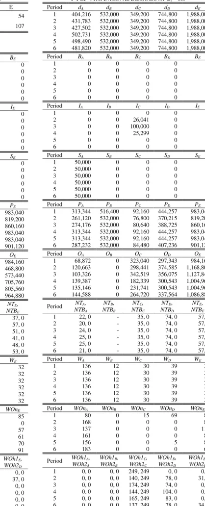
TABLE VII
P-FGP WITH INTERVAL DEMANDSAT 1 = 0.8
Period dA dB dC dD dE
1 404,216 532,000 349,200 744,800 1,988,000 2 431,783 532,000 349,200 744,800 1,988,000 3 427,502 532,000 349,200 744,800 1,988,000 4 502,731 532,000 349,200 744,800 1,988,000 5 498,490 532,000 349,200 744,800 1,988,000 6 481,820 532,000 349,200 744,800 1,988,000
Period BA BB BC BD BE
1 0 0 0 0 0
2 0 0 0 0 0
3 0 0 0 0 0
4 0 0 0 0 0
5 0 0 0 0 0
6 0 0 0 0 0
Period IA IB IC ID IE
1 0 0 0 0 0
2 0 0 26,041 0 0
3 0 0 100,000 0 0
4 0 0 25,299 0 0
5 0 0 0 0 0
6 0 0 0 0 0
Period SA SB SC SD SE
1 50,000 0 0 0 0
2 50,000 0 0 0 0
3 50,000 0 0 0 0
4 50,000 0 0 0 0
5 50,000 0 0 0 0
6 50,000 0 0 0 0
Period PA PB PC PD PE
1 313,344 516,400 92,160 444,257 983,040 2 261,120 532,000 76,800 370,215 819,200 3 274,176 532,000 80,640 388,725 860,160 4 313,344 532,000 92,160 444,257 983,040 5 313,344 532,000 92,160 444,257 983,040 6 287,232 532,000 84,480 407,236 901,120
Period OA OB OC OD OE
1 68,872 0 323,040 297,343 984,160 2 120,663 0 298,441 374,585 1,168,800 3 103,326 0 342,519 356,075 1,127,840 4 139,387 0 182,339 300,543 1,004,960 5 135,146 0 231,741 300,543 1,004,960 6 144,588 0 264,720 337,564 1,086,880
Period NTA, NTBA
NTB, NTBB
NTC, NTBC
NTD, NTBD
NTE, NTBE
1 22, 0 - 35, 0 74, 0 57, 0
2 20, 0 - 35, 0 74, 0 57, 0
3 24, 0 - 35, 0 74, 0 57, 0
4 25, 0 - 35, 0 74, 0 57, 0
5 25, 0 - 35, 0 74, 0 57, 0
6 21, 0 - 35, 0 74, 0 57, 0
Period WA WB WC WD WE
1 136 12 30 39 32
2 136 12 30 39 32
3 136 12 30 39 32
4 136 12 30 39 32
5 136 12 30 39 32
6 136 12 30 39 32
Period WOnA WOnB WOnC WOnD WOnE
1 80 0 15 69 85
2 168 0 0 0 81
3 137 0 0 0 112
4 161 0 0 0 87
5 156 0 0 5 87
6 183 0 0 0 66
Period WOh1A, WOh2A
WOh1B, WOh2B
WOh1C, WOh2C
WOh1D, WOh2D
WOh1E, WOh2E
1 0, 0 0, 0 249, 249 0, 0 0, 0 2 0, 0 0, 0 140, 249 78, 0 31, 0 3 0, 0 0, 0 174, 249 74, 0 0, 0 4 0, 0 0, 0 144, 249 104, 0 0, 0 5 0, 0 0, 0 165, 249 83, 0 0, 0 6 0, 0 0, 0 137, 249 78, 0 34, 0 PIS1 = 229,058,460 Baht, PIS2 = 0 worker, NIS1 = 136,687,324 Baht, NIS2 = 52 workers, = 92,371,135, = 52,2 = 0.99.
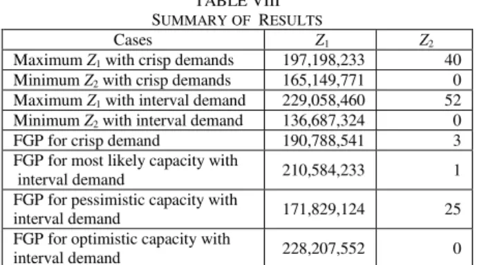
Using the proposed P-FGP model with interval demand, Decision Maker (DM) can set the satisfaction level of the first objective that can be alleviated and then the best solution can be found at high degree of satisfaction level (ex. =0.8, ) for most-likely case, which is better than single objective optimization and multiple objective optimization with crisp demand. The proposed model is better than single objective optimization due to consideration of both goals under acceptable level of the first goal. It also has advantages over multiple objective optimization problems with crisp demands. In this study P-FGP with crisp demand and interval demand are compared. In the first goal, profit is increased from 190,788,541 to 210,584,233 Baht and change of workforce level is reduced from 3 to 1 worker. These advantages exist because all of backorder quantities are eliminated and transportation cost for backorder is also eliminated. The total workforce level for P-FGP with interval demands is fewer than the total workforce level for P-FGP with crisp demands. Hiring and firing is also fewer. So, costs related to workforce level are reduced and change of workforce level is also reduced. However, inventory level for P-FGP with interval demands is greater than inventory level for P-FGP with crisp demands. These benefits can be occurred because the appropriate demands are selected from possible demand intervals for generation the APP. The results of decision variables are shown in Table VI, VII. In the proposed model fuzzy capacity is also considered so additional results of pessimistic and optimistic cases can be generated that. This information can help DM to decide the production plan when the situation changes. The results for each case are shown in Table VIII.
TABLE VIII
SUMMARYOF RESULTS
Cases Z1 Z2
Maximum Z1 with crisp demands 197,198,233 40 Minimum Z2 with crisp demands 165,149,771 0 Maximum Z1 with interval demand 229,058,460 52 Minimum Z2 with interval demand 136,687,324 0 FGP for crisp demand 190,788,541 3 FGP for most likely capacity with
interval demand 210,584,233 1
FGP for pessimistic capacity with
interval demand 171,829,124 25
FGP for optimistic capacity with
interval demand 228,207,552 0
IV. CONCLUSION
Preemptive fuzzy goal programming (P-FGP) model for aggregate production and logistics planning with interval demand and uncertain production capacity is proposed for solving the problem of the case study. Two fuzzy goals; profit goal and change of workforce level goal were considered. P-FGP model with interval demand has advantages over single objective optimization and P-FGP model with crisp demands because the better solution can be found for both profit and change of workforce level by setting the appropriate demand from a possible demand interval. P-FGP with interval demand can reduce costs of backorder, transportation, hiring, firing and subcontract. The fuzzy production capacity is also considered. Three models of P-FGP are generated based on optimistic, pessimistic and most-likely criteria. These can give more information for
DM when the situation changes.
Further study might consider uncertainty of cost coefficients. Interactive approach is also attractive for DMs.
REFERENCES
[1] R. Chen Wang and T. Fu Liang, ―Application of fuzzy multi-objective
linear programming to aggregate production planning,‖ Computers & Industrial Engineering, vol. 46, pp. 17–41, 2004.
[2] M. Belmokaddem, M. Mekidiche and A. Sahed, ―Application of a fuzzy goal programming approach with different importance and
priorities to aggregate production planning,‖ Journal of applied quantitative methods, vol. 4, no. 3, pp. 317-331, 2009.
[3] C. Gomes da Silva, J. Figueirab, J. Lisboab, and S. Barmane, ―An interactive decision support system for an aggregate production planning model based on multiple criteria mixed integer linear programming,‖ International Journal of Management Science, Omega 34, pp. 167 – 177, 2006.
[4] S.Eilon, ―Five Approaches to Aggregate Production Planning,‖ AIIE T., vol.7, no. 2, pp.118-131, 1975.
[5] D.A. Goodman, ―A New Approach to Scheduling Aggregate Production and Workforce,‖AIIE T., vol. 5, no. 2, pp.135-141, 1973. [6] Abu S.M. Masud, and C.L. Hwang, ―Aggregate Production Planning
Model and Application of Three objective Decision Methods,‖
Ind.J. of Prod. Res.,‖ vol. 8, no. 6, pp. 741-752, 1980.
[7] J. P. Ignizio, Linear programming in single- & multiple-objective system. USA: Prentice-Hall, Inc., 1982.
[8] Stephen C. H. Leung, Yue WU and K. K. Lai, ―Multi-site aggregate production planning with multiple objectives: a goal programming
approach,‖ Production Planning & Control, vol. 14, no.53, pp. 425– 436, July-August 2003.
[9] Stephen C. H. Leung and Wan-lung Ng, ―A goal programming model
for production planning of perishable products with postponement,‖
Computers & Industrial Engineering, vol.53, pp. 531–541, 2007. [10] Stephen C. H. Leung and Shirley S.W. Chan, ―A goal programming
model for aggregate production planning with resource utilization
constraint,‖ Computers & Industrial Engineering, vol.56, pp. 1053– 1064, 2009.
[11] H. Rommelfanger, ―Interactive Decision Making in Fuzzy Linear
Optimization Problems,‖ Eur. J. Oper. Res., vol. 41, pp. 210-217, 1989.
[12] A. Baykasoglu and T. Gocken, ―Multi-objective aggregate production
planning with fuzzy parameters,‖ Advances in Engineering Software, vol.41, pp. 1124–1131, 2010.
[13] C.N.Cha and H.Hwang, ―Experimental Comparison of the Swithing Heuristics for Aggregate Production Planning Problem,‖Computers & Industrial Engineering, vol.31, no.3/4, pp. 625-630, 1996. [14] H. J. Zimmermann, ―Fuzzy Programming and Linear Programming
with Several Objective Functions,‖ Fuzzy Sets and Syst., vol. 1, pp. 45-55, 1977.
[15] H. J. Zimmermann, Fuzzy sets and systems 1. USA: North Holland Publishing Company, 1978.
[16] H. J. Zimmermann, Fuzzy Set Theory and Its Applications. 4th ed., USA: Kluwer Academic Publishers, 2001.
[17] R. Y. K. Fung, J. Tang and D. Wang, ―Multiproduct Aggregate
Production Planning With Fuzzy Demands and Fuzzy Capacities,‖
IEEE Transactions on systems, man, and cybernetics - Part A: Systems and humans, vol. 33, no. 3, pp. 302 -313, May 2003. [18] W. Zhu, ―The application of fuzzy programming to the aggregate
production planning-markdown pricing problem,‖ in The 7th Int. Symposium on Operations Research and Its Applications, pp. 457– 464, October 31 - November 3, 2008.
[19] G. Biyik, B. Gülsün and D.Özgen, ―A fuzzy set theory application for aggregate production planning in the presence of both demand and
capacity vagueness,‖ in 35th Int. Conf. on Computers and Industrial Engineering, pp. 297-302, 2005.
[20] W.Nunkaew and B.Phruksaphanrat, ―A Fuzzy Multiple Objective Decision Making Model for Solving a Multi-Depot Distribution
Problem,‖ in Proceedings of the Int. MultiConf. of Engineers and Computer Scientists 2010, Hong Kong, pp. 1890-1896, 2010. [21] Y. Jou. Lai and C. Lai. Hwang, Fuzzy multiple objective decision
making: Methods and Applications. Great Britain: Springer-Verlag Berlin Heidelberg, 1994
[22] R. Chen Wang and T. Fu Liang, ―Applying possibilistic linear
programming to aggregate production planning,‖ International Journal of Production Economics, vol. 98, pp. 328–341, 2005. [23] Wang, A course in fuzzy system and control, International Ed., USA: