The dynamic behaviour of budget components and output – the cases of France, Germany, Portugal, and Spain

The dynamic behaviour of budget components

and output – the cases of France, Germany,

Portugal, and Spain

±

António Afonso,

* #

Peter Claeys

$

October 2006

Abstract

The main focus of this paper is the relation between the cyclical components of total revenues and expenditures and the budget balance in France, Germany, Portugal, and Spain. We try to uncover past trends behind the development of public finances that contribute to explaining the current stance of fiscal policy. The disaggregate analysis of fiscal policy in an SVAR that mixes long and short-term constraints allows us to look into the transmission channels of fiscal policy and to derive a model-based indicator of structural balance. The main conclusions are that fiscal slippages are mainly due to reversals in tax policies, which are unmatched by expenditure adjustments. As a consequence, deficits rise when economic conditions worsen but cause a ‘ratcheting up’ in the size of government in economic booms. The Stability and Growth Pact has not eradicated these procyclical policies. Bad policies in good times also contribute to aggregate macroeconomic instability.

Keywords: fiscal indicator, structural balance, output gap, SGP, EMU, SVAR, short and

long-term restrictions.

JEL Classification Numbers: E62, E65, E66, H61, H62.

± _{We are grateful to Luís Costa, Arne Gieseck, Michael Thöne, Jürgen von Hagen, Jan in't Veld, seminar}

participants at the ECB (Frankfurt), at ISEG/UTL (Lisbon), at the 61ST

European Meeting of the Econometric Society (Vienna), and at the DG ECFIN workshop on Fiscal Indicators for EU Budgetary Surveillance (Brussels) for helpful comments and discussions. Valuable assistance of Renate Dreiskena with the data is highly appreciated. The opinions expressed herein are those of the authors and do not necessarily reflect those of the ECB or the Eurosystem. Peter Claeys thanks the Fiscal Policies Division of the ECB for its hospitality.

*

European Central Bank, Kaiserstraße 29, D-60311 Frankfurt am Main, Germany, email: antonio.afonso@ecb.int.

#

ISEG/UTL - Technical University of Lisbon, Department of Economics; UECE – Research Unit on Complexity in Economics, R. Miguel Lupi 20, 1249-078 Lisbon, Portugal. UECE is supported by FCT (Fundação para a Ciência e a Tecnologia, Portugal), under the POCTI program, financed by ERDF and Portuguese funds. email: aafonso@iseg.utl.pt.

2

Contents

1. Introduction... 3

2. The recent fiscal imbalances in the EU ... 4

3. An SVAR model for gauging fiscal indicators ... 6

3.1. Fiscal indicators ... 6

3.2. Towards an economic indicator of fiscal policy... 8

3.3. Methodology ... 10

3.4. Gauging the fiscal indicator ... 14

4. Empirical analysis... 16

4.1. Data ... 16

4.2. The transmission channels of fiscal policy... 18

4.3. The fiscal indicator... 22

4.4. Some sensitivity analysis... 25

5. Conclusion... 29

References ... 31

Appendix 1. Data sources ... 46

Appendix 2. The fiscal indicator: some additional results... 47

3

1. Introduction

In recent years, we have witnessed a worldwide swing towards fiscal profligacy. In the

European Union, this has come somewhat as a surprise as the Maastricht Treaty and

afterwards the Stability and Growth Pact seemed to have put in place a set of fiscal rules

that guarantee the sustainability of public finances. The difficulty in applying the Pact, first to

Portugal and later on to France and Germany, has been followed by a more widespread

breach of the 3% deficit limit in several EU countries. A revised version of the Pact was

adopted in March 2005, and takes a more flexible approach in terms of curbing excessive

deficits over a longer period of time, and pays more attention to sustainability of public

finances. As part of the Lisbon Strategy, considerably more attention is given to the

composition of budget adjustments with a view to promoting economic growth.

A variety of political and economic factors probably underlie the observed rise in public

deficit and debt ratios. We try to uncover any underlying past trends behind the development

of public finances that may contribute to explaining recent budgetary outlook in France,

Germany, Portugal, and Spain. While the first three countries were subject to several steps

of the Excessive Deficit Procedure, Spain on the other hand could be seen as an example of

more vigorous fiscal management. We are particularly interested in the underlying causes of

the breach of the Pact’s rules by looking into adjustments in various budget components. At

the same time, we look into how these adjustments contribute to the long-term growth

prospects and outlook for the sustainability of public finances.

To that end, we construct a model-based indicator of structural balance by combining

insights from the growing empirical literature on the effects of fiscal policy – modelled with

structural VARs – with statistical methods for cyclically adjusting fiscal balances. Our

approach innovates on extant evidence in using a mixture of short and long-term restrictions

to identify economic and fiscal shocks in a small-scale empirical model in economic growth

and fiscal variables. This allows for permanent shocks to determine trending behaviour of

output and fiscal variables à la Blanchard and Quah (1989). Discretionary fiscal adjustments

are captured by filtering out the fiscal balance for cyclical reactions of budget items, following

Blanchard and Perotti (2002).

The quantitative indicator that we obtain is best seen in the light of the growing theoretical

literature on the qualitative effects of fiscal policy. Dynamic stochastic general equilibrium

models with nominal rigidities search for a rationale for fiscal stabilisation policies. At the

4

and demand side effects of fiscal policy adjustments. Our indicator is consistent with such a

distinction. We take a first step by restricting attention to overall expenditure and revenues,

but more elaborate models might incorporate refinements in the compositional adjustments

of budget balance. In contrast to statistical models for adjusting fiscal balance, our economic

indicator of structural balance has some attractive practical properties. Uncertainty is

explicitly quantified, and theoretical assumptions can be explicitly tested. Also, the

end-of-sample problem is reduced. The model is not necessarily more demanding in terms of data

availability.

The main result of our study is that both pre-EMU consolidations and expansions in recent

years are mainly based on revenue changes. The derailing of public finances comes from

tax reductions being implemented in good economic times. As total revenues apparently

remain constant, spending cuts are not implemented. As a consequence, deficits show up

again when economic boom turns into bust. The easy way out of deficits is to reverse

previous tax cuts, leading to a ‘ratcheting up’ of spending over the next economic cycle. This

procyclical bias in fiscal policies has not been eliminated with the Stability and Growth Pact.

Governments still implement bad policies in good times. These policy reversals have

negative economic effects. We find fiscal policy to have minor supply but large demand

effects. Procyclical policies unnecessarily induce macroeconomic fluctuations.

The remainder of the paper is organised as follows. In section two, we briefly review some

recent fiscal developments in the EU, notably for the cases of France, Germany, Portugal,

and Spain. Our structural VAR approach towards disentangling these developments, and the

derivation of the fiscal indicator, is discussed in section three. Section four reports our

empirical results, and section five concludes the paper.

2. The recent fiscal imbalances in the EU

The fiscal framework of EMU has been considered a means for implementing fiscal

consolidation. However, recent developments in several Euro Area countries raise the

question as to whether fiscal sustainability is endangered, in view of rising deficits and debts

at a moment when the effects of ageing populations will have a further burdening effect. In

2005, Excessive Deficit Procedures (EDP) have been carried out for both France and

Germany, while yet another EDP was launched for Portugal. There are also ongoing

5

excessive deficit.1 Recent developments cannot be seen without taking into account past

actions and trends in public finances.2 We focus attention on the evolution of public finances

since 1970 in the countries that initially ’sinned’ to the Pact (France, Germany and Portugal).

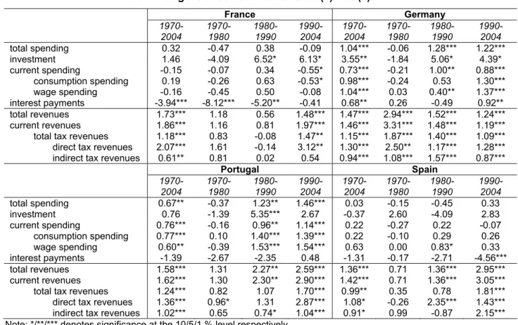
We report in Figure 1 the general government balance, and its breakdown in revenue and

expenditure ratios. A simple visual inspection shows that expenditure and revenue ratios

have been following an increasing trend notably in France, Portugal and Spain. But with

revenues lagging the expenditure rises, there has been a continuous deficit bias. There were

some good reasons in 1991 to embark on consolidation by enshrining the 3% deficit target in

the criteria for EMU-entry. The Maastricht rules have been effective in constraining further

buoyant expenditure rises. Less than commensurate rises in revenue intake have led to

persistent albeit gradually declining deficits. Since the start of EMU, fiscal positions have

started to slip away again. As to the reasons for the breach of the Stability and Growth Pact,

further expenditure rises in France and Portugal seem to blame, whereas in Germany large

revenue reductions unmatched by expenditure cuts have pushed the deficit beyond the 3%

threshold. Spain, on the other hand, stands out for its balanced budget over recent years,

which is the result of a sustained reduction in expenditures since 1993 that has levelled off in

recent years. We consider Spain as an example of more prudent fiscal behaviour.

[INSERT FIGURE 1 HERE]

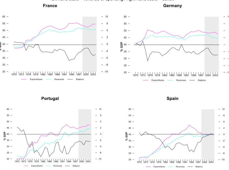
These budget developments cannot be separated from economic conditions. The balance

can slip out of the control of fiscal authorities by higher than expected expenses on

unemployment benefits and transfers, or less than budgeted revenues, owing to automatic

stabilisers. Figure 2 compares some measures of the output gap and cyclically adjusted

balances computed by the European Commission and the OECD, as well as a trend series

retrieved from directly applying a Hodrick-Prescott filter on the raw series.3

[INSERT FIGURE 2 HERE]

The start-up of the EDPs to these countries seems justified on account of worsening

structural balances. In all countries, economic conditions improved considerably at the onset

of EMU and the overall deficit was notably reduced as a result. But the reversal of positive

output gaps laid out the structural weakness of the balance in France, Germany and

1 _{The other countries that faced an EDP are the Netherlands, Slovakia, Poland, Malta, Hungary, Cyprus and the}

Czech Republic. For further details see the EC web site at:

http://europa.eu.int/comm/economy_finance/about/activities/sgp/procedures_en.htm.

2 _{Afonso (2005) questions the sustainability of public finances in most EU countries.} 3

6

Portugal. Expenditures exceed average revenues over the cycle. In contrast, Spain presents

an entirely different picture. The budget has been brought close to balance, and is even in

slight surplus. A constant spending share has been matched by gradually rising tax

revenues.

3. An SVAR model for gauging fiscal indicators

There are a variety of reasons for which the cyclically adjusted balance does not properly

reflect discretionary shifts under the control of the government. Its use in assessing fiscal

balances is therefore debatable. Some problems are related to the properties of the

econometric filters that are being used.4 _{More importantly, we believe fiscal policy}

contributes to the size of economic fluctuations. And it does so by adjusting a variety of

spending and revenue items. Recent general equilibrium theories of fiscal policies provide a

rationale for real economic effects of fiscal policies, and stress the prevalence of its

supply-side consequences over short-term demand effects. This is all the more important for the

assessment of the new Stability and Growth Pact. We develop an indicator of discretionary

fiscal policy stance that builds on the recent empirical literature on the effects of fiscal policy

using structural VARs, and combine this with evidence on the cyclical behaviour of

government budget. Next to its favourable properties, the indicator is best seen as a first

step in verifying recent theories of fiscal policy as well as giving an instrument for assessing

the quality of fiscal adjustments.

3.1. Fiscal indicators

The notion of structural balance is based on the premise that total output fluctuates around

some unobserved trend that depends on the long-term potential growth path of the

economy. In combination with some assumptions on the cyclical behaviour of fiscal policy,

this allows deriving a cyclically adjusted balance. Common practice at the European

Commission, IMF or OECD regards the determination of cyclical variation in output and the

cyclicality of the budget as two distinct problems.

First, the output gap usually comes from some trend-extraction procedure with a statistical

filter applied directly to real output. This decomposition in trending and cyclical components

is usually done with a band-pass filter. Alternatively, the output gap is calculated as the

distance from actual to potential output where the latter is based on a production function for

7

the aggregate economy.5 Second, a bottom-up approach is adopted for the derivation of the

cyclical elasticities of the budget. The output elasticities of government revenues are based

on the taxation structure of each main sub-item6 – in some cases accounting for collection

lags – and the elasticity of the tax bases to output. The spending elasticity is of relatively

minor importance, as only the spending on unemployment benefits is adjusted for the cycle.

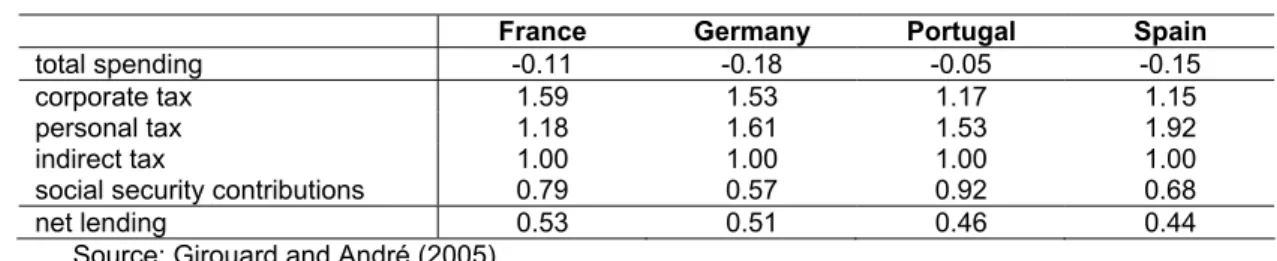
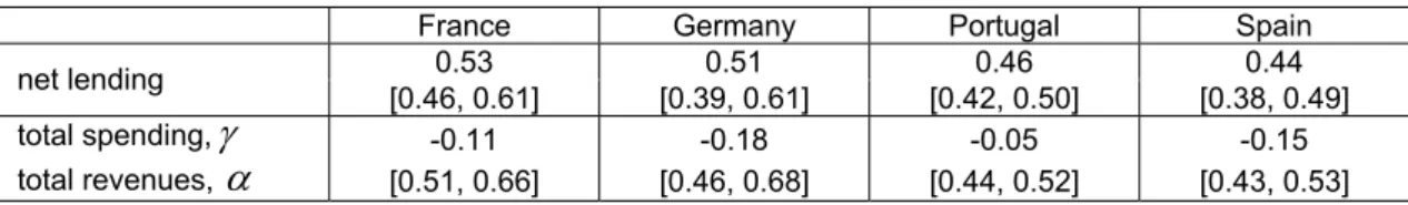
Other budget components are assumed to be cyclically insensitive. Table 1 gathers the

elasticities from OECD for the major budget categories in the countries we study.7 As in

most other European countries, the cyclical elasticity of total net lending varies around 0.50.

Most of the variation in the budget comes from procyclical corporate and personal taxes.

Table 1. OECD output elasticities of various budget items

France Germany Portugal Spain

total spending -0.11 -0.18 -0.05 -0.15

corporate tax 1.59 1.53 1.17 1.15

personal tax 1.18 1.61 1.53 1.92

indirect tax 1.00 1.00 1.00 1.00

social security contributions 0.79 0.57 0.92 0.68

net lending 0.53 0.51 0.46 0.44

Source: Girouard and André (2005).

Quite some uncertainty surrounds the computation of structural balances in this two-step

procedure. Depending on the skewness of the distribution of the moving-average weights in

the filter that is being applied and the phase of the economic cycle, trend output is biased

towards actual values especially towards the end of the sample. Another problem is posed

by structural breaks. Windfall revenues or unexpected spending are entirely included in the

structural balance if they have no economic effects. Filters distribute the effects of a break

forward and backward on the trend. But this problem is not limited to statistical methods.

Even if we use the production function or consider a deterministic trend a reasonable

approximation to potential output, incorporating shifts remains a problematic issue. The

production function approach moreover suffers from plenty of assumptions that make

cumulative uncertainty rather large.8 _{The various assumptions on budget elasticities are not}

as crucial for the cyclically adjusted balance, but are nevertheless not less problematic.

Implicitly, it is assumed that average budget elasticities have a time-invariant linear relation

5 _{The European Commission backs up a Hodrick-Prescott based decomposition with results from the production}

function approach (European Commission, 1995). The OECD uses only the production function method (Giorno et al., 1995). The IMF has no uniform strategy but the production function method prevails for industrialised countries (IMF, 1993). Many other approaches abound. Methods that use a Beveridge-Nelson decomposition or track output developments with unobserved components are less common. Blanchard (1993) asks what the primary surplus would have been, had the unemployment rate remained the same as the previous year. Chouraqui et al. (1992) compare different moving benchmarks. Cohen and Follette (2000) use spectral analysis to isolate low frequency changes in fiscal policy.

6 _{The OECD adjusts only social security contributions, corporate, personal and indirect taxes.}

7 _{Girouard and André (2005) update the elasticities in a previous OECD study by Van den Noord (2002).} 8

8

to changes in the economy. We return to these difficulties in a sensitivity analysis in section

4.4.

3.2. Towards an economic indicator of fiscal policy

The main difficulty in interpreting the structural balance is the absence from economic

arguments to underpin the trend/cycle decomposition. There is an implicit assumption in the

filtering methods on the frequency of the business cycle and hence on trend output under

average economic conditions. And while the production function approach builds upon

economic foundations, the dynamics are nonetheless driven solely by the longer-term

effects of investment feeding back on changes in the capital stock.9

Macroeconomic models that allow for cyclical fluctuations around some steady-state

trending growth path can be found in the growing class of Dynamic Stochastic General

Equilibrium (DSGE) models with nominal rigidities. These models have by now been

extended to include fiscal policy. In the initial Real Business Cycle models, there are only

supply-side effects of fiscal policy that transmit through wealth effects and the labour/leisure

choice (Baxter and King, 1993). Micro-founded models based on sticky prices provide a

rationale for stabilisation policies, but even in the New Keynesian type of models of fiscal

policy, the supply side effects still tend to dominate demand side effects of fiscal policy

management (Linnemann and Schabert, 2003). A larger role for demand side effects of

fiscal policy is only found in models that introduce some further imperfections via ‘Rule of

Thumb’ consumers or a fraction of liquidity constrained consumers (Galí et al., 2005; Bilbiie

et al., 2006). The latter models come also closer to replicating the results of the growing

empirical literature on the effects of fiscal policy.

The main result of studies that use the VAR-counterparts to DSGE-models is that they can

indeed recover significant effects of fiscal expansions on output. These are more in line with

a positive ‘Keynesian’ effect on consumption, albeit the eventual multiplier is strongly

reduced. The identification of fiscal policy is fraught with difficulties, however.10 First, the

implementation of announced changes in government policies is subject to lengthy and

visible political negotiations that are anticipated in private agents’ behaviour. As a

consequence, fiscal shocks need not affect fiscal variables first. This is a problem of the

shock being non-fundamental (Lippi and Reichlin, 1994). Second, decisions on fiscal policy

affect different groups in the public via a range of different spending and tax instruments.

There exists no ‘standard’ fiscal shock: every political discussion considers the trade-off

9

Potential output is nevertheless assumed exogeneous in the production function approach.

9

between a range of possible taxation and spending adjustments. The means of financing

and the adjustment in expenditures and revenues wrap empirically relevant effects of

different budget components in an aggregate fiscal shock without considering the path of

public debt. Most studies focus on total spending or revenues, and find small and positive

effects of government spending on consumption, but prolonged negative effects of higher

taxation. Only a couple of studies consider the dynamic behaviour of some particular budget

components.11 Third, these identification problems are only exacerbated by the automatic

reaction of fiscal aggregates to economic variables.

The seminal contribution of Blanchard and Perotti (2002) lies in using a semi-structural VAR

that employs external institutional information on the elasticity of fiscal variables to output.

Cleaning out the automatic cyclical reaction of the total fiscal balance leaves shifts to the

cyclically adjusted balance as discretionary fiscal shocks. Blanchard and Perotti (2002)

additionally impose some timing restrictions on the economic effects of discretionary policy.

These timing assumptions avoid to some extent anticipation effects but would not capture

these completely if implementation lags are important. Subsequent studies have mainly

attempted to verify the original approach of Blanchard and Perotti (2002) with a variety of

techniques and usually tend to confirm their findings.12

However, the empirical literature has hitherto ignored the supply and demand channels of

fiscal policy that are at front-stage of the theoretical DSGE models. Such effects are only

implicitly acknowledged in these VAR studies. Changes in tax revenues, for example, are

usually found to have lasting effects on output. There are nevertheless two other strands of

the empirical fiscal policy literature that attribute a role to supply side variables. First, the

literature on non-Keynesian effects of fiscal policy would argue that fiscal consolidation

might have positive consequences on output. The composition of the fiscal adjustment

thereby plays an important role (Alesina and Perotti, 1995). The effects of consolidation on

agents’ expectations on the future economic outlook – measured by asset markets’ reaction

(Giavazzi and Pagano, 1990) – suggests a role for permanent wealth and supply-side

effects of fiscal policy. Second, most VAR studies have so far ignored the literature on the

long-term growth effects of fiscal policies. The main message of the endogenous growth

models that have been developed is that higher taxation unambiguously reduces output, but

11 _{Ramey and Shapiro (1998) look into the sectoral reallocation effects following shocks. A particular role in the}

transmission of fiscal policy shocks is also played by the labour market. A couple of papers compare the effects of consumptive government purchases to increases in public employment (Finn, 1998; Pappa, 2005; Cavallo, 2005). Perotti (2004) and Kamps (2004) examine the output and labour market effects of government investment.

12 _{Mountford and Uhlig (2002) retrieve different types of fiscal shocks among those that conform to some a priori}

10

that these losses may be offset by using the proceeds for productive spending items (Barro,

1990; King and Rebelo, 1990). These seminal models have been made more realistic by

allowing endogenous responses of labour (Turnovsky, 2000). Typical tests of these growth

models give empirical support to the role of spending and taxes to long-term growth (Kneller

et al., 1999). It can be argued that additional government spending in catching-up countries

such as Portugal and Spain had rather different effects than further expansions of the

budget in France and Germany, for example. This provides an additional argument for

including the former countries in our analysis.

The examination of the growth effects is also of substantial policy interest. In the

assessment of EU Member States’ policies under the revised Stability and Growth Pact,

much attention is devoted to the quality of fiscal adjustments and the sustainability of public

finances. The implementation of major structural reforms that raise potential growth – and

hence have an impact on the long-term sustainability of public finances – can be considered

grounds for temporary deviations of budget balance. There is thus need for a framework that

assesses changes in fiscal instruments and distinguishes the short-term demand from the

longer run supply effects of such policies.

3.3. Methodology

We make a first step in setting up an empirical VAR model that allows for fiscal policy having

distinct long- and short-term effects on output. The approach in this paper rests on a

combination of long-term restrictions and some assumptions on the short-run elasticities of

budgetary items.13 _{For the purpose of gauging a model-based fiscal indicator, we basically}

take shocks with permanent effects on output to drive long-term trends. Following Blanchard

and Quah (1989), potential output is determined by so-called productivity or technology

shocks that permanently affect output. This can then be complemented with further

assumptions on the short-term behaviour of fiscal policies. Shocks with transitory output

effects are classified as either cyclical or fiscal, following the elasticity approach of Blanchard

and Perotti (2002).

13 _{There are a few applications of fiscal VARs that use similar restrictions, and are mostly inspired by a practical}

11

We specify an empirical model of fiscal policy as a small-scale VAR in real output

y

_t and the expenditure

g

_t and revenue side

t

_t of the government budget. We can summarise the data properties in a VAR-model (1), ignoring for ease of notation any deterministic terms:

t t

X

L

B

(

)

=

ε

(1)

where

X

_t refers to the vector of variables

[

y

_t

g

_t

t

_t

]

, and

ε

_t contains the reduced form OLS-residuals. By rewriting the VAR into its Wold moving average form (2),

t t

B

L

X

=

₍

₎

−1

ε



t

′



t

 

. (2)

and imposing some structure on the relation between reduced form residuals

ε

_t and structural shocks

η

_t via the transformation matrix

A

(such that

A

ε

_t

=

η

_t), we can write the model (2) as follows:

t t

t

C

L

B

L

A

X

=

(

)

η

=

(

)

−1

ε



t ′



t



I

. (3)

Any SVAR analysis needs to impose at least as much restrictions as contained in the matrix

A

to identify the model. By imposing orthogonality of the structural shocks we have already

six (i.e. the covariance matrix of OLS residuals

Ω

=

AA

'

). Hence, we need to choose at least three more restrictions. The ones we employ are a combination of long and short-term

restrictions. The latter shape the contemporaneous relations among the variables through a

direct parameter choice on

A

. The former impose a long-term neutrality constraint on the

effects of a structural shock

j

on some variable

i

. That is, the i,j-th element of the infinite

horizon sum of coefficients, call it

C

(

1

)

_ij, is assumed to be zero. This requires an indirect restriction in (3) on the product of the transformation matrix

A

and the inverted long-run

coefficient matrix

B

(

1

)

−1. In other words,

[

C(1)

]

_ij =

[

B(1)−1A

]

_ij =0. (4)

For the system consisting of government expenditures, revenues and output, we assume

12

long-term trend rise in output and leads to the unit root behaviour of real output. This shock

is isolated by assuming there are two further shocks in the model that both have temporary

effects on output. I.e., we assume that

[

C

(

1

)

]

₁₂

=

0

and

[ ]

C

(

1

)

₁₃

=

0

in (4). These shocks can

be interpreted respectively as a generic business cycle shock (

η

c_{) capturing short-term}

fluctuations around the moving steady state equilibrium for output, and a fiscal shock (

η

f) with short-term ‘demand’ effects on output. In order to distinguish the business cycle shock

from that to fiscal policy, we employ the elasticity approach advocated by Blanchard and

Perotti (2002). We derive a shock to spending and/or revenues from which the cyclical

effects have been removed. In other words, the shock with transitory effects on output – but

unaffected by short-term variation in output – is the fiscal policy shock and reflects

discretionary changes in the fiscal policy stance.14 We take elasticities for government

expenditures (

γ

) and revenues (

α

) with respect to output, and impose these values on the

relation in

A

between the reduced form residuals for output (

ε

y) and spending (

ε

g) respectively revenues (

ε

t_).15

The fiscal shock thus includes discretionary decisions

unrelated to the cycle. Moreover, any government policy that interferes with the workings of

automatic stabilisers on a systematic basis is considered as a fiscal intervention. Unlike

other VAR studies, we split an overall change in fiscal policy into a part that has a short-term

economic effect (the fiscal ‘demand’ shock), and into shocks that may have potentially

long-term growth effects (the ‘supply’ shock).16

One important limitation of the current version of the model is that we cannot tell apart the

growth effects coming from ‘pure’ technology shocks from those deriving from tax and

spending decisions. Our supply shock is thus a combination of all shocks with long-term

output effects. The negative effects of distortionary taxation or incentive-distorting spending

show up in this shock, as well as the possibly positive effects of government investment.

Instead, we isolate in the fiscal ‘demand’ shock only those changes in the discretionary

budget stance that have temporary effects on output. A full-fledged analysis of the economic

growth effects of fiscal policy would require additional restrictions.17 _{The current identification}

14 _{This is not a replication of the results in Blanchard and Perotti (2002) as they require additional short-term}

constraints on the timing of the effects whereas we consider long-term constraints.

15 _{We therefore need to impose two different coefficients}

γ

_and

α

_{which results in one overidentifying}

restriction. Blanchard and Perotti (2002) instead net out the cyclically sensitive transfers from spending, and assume a zero elasticity on other spending categories. As the sensitivity analysis in section 4.4 demonstrates, this does not seem to affect our results.

16 _{For this reason, we do not expect responses to our fiscal shock to be similar to those documented in the}

empirical literature. Our distinction is more consistent with the theoretical models of fiscal policy.

17 _{We make some suggestions in the concluding section. We considered the effect of loosening the long-term}

13

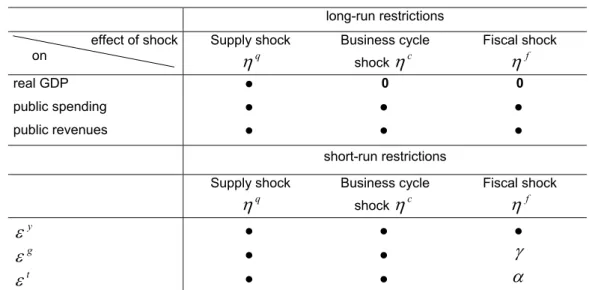
is sufficient though for the purpose of deriving a fiscal indicator. We summarise our

assumptions in (5) (see also Table 2):

⎥ ⎥ ⎥ ⎦ ⎤ ⎢ ⎢ ⎢ ⎣ ⎡ • • • • • • • = 0 0 ) 1 (

C and

⎥ ⎥ ⎥ ⎦ ⎤ ⎢ ⎢ ⎢ ⎣ ⎡ • • • • • • •

=

γ

α

A . (5)

We can not simply set to zero the elasticity

γ

of government expenditures. Unemployment

benefits move over the cycle in EU-countries, even if their contribution to variation in total

spending is not large. The parameter

γ

comes directly from the elasticities calculated by the

OECD that we reported in Table 1. Instead of multiplying each revenue category by its

cyclical elasticity and GDP share, we have subtracted the spending elasticity (row 2 in Table

1) – accounting for its share in GDP – from the elasticity of total net lending (row 7 in Table

1) so as to obtain the total elasticity of revenues

α

. The coefficients do not sum to zero as

the budget is assumed to be countercyclical. Table 3 summarises our parameter

assumptions.

Table 2. Identification in the long- and short-term

long-run restrictions

effect of shock on

Supply shock

q

η

Business cycle shock

η

c

Fiscal shock

f

η

real GDP

•

0 0

public spending

•

•

•

public revenues

•

•

•

short-run restrictions Supply shock

q

η

Business cycle shock

η

c

Fiscal shock

f

η

y

ε

•

•

•

g

ε

•

•

γ

t

ε

•

•

α

Table 3. Parameters

γ

and

α

France Germany Portugal Spain

total spending

γ

-0.11 -0.18 -0.05 -0.15

14

3.4. Gauging the fiscal indicator

The structural model then permits adopting a unified approach towards contemporaneously

uncovering indicators of potential output *

y

and the structural balance *

d

. Basically, total

output and government expenditures and revenues can be decomposed into the contribution

of each of the structural shocks. We take the stance that only supply shocks determine

potential output y_t* in the long term. Both fiscal shocks and supply shocks determine structural expenditure g_t* and revenues t_t*.18 Under this assumption, one can compute the structural deficit as in (6):

* * * *

t t t t

y t g

d = − . (6)

This fiscal indicator

d

* can be interpreted as reflecting the discretionary stance of the fiscal

authority. From the decomposition of the budget, we can then analyse whether such

changes usually occur via spending or taxation measures.

This measure cannot directly be compared to the cyclically adjusted balances provided by

the European Commission, the OECD or to those derived from some statistical filtering

method. First, the output gap we derive need not correspond to the fluctuations around a

smooth trend on some assumption on the frequency of the business cycle. The economic

shocks that drive potential output reflect changes in productivity – that may derive from a

variety of sources – and might vary over time. Our approach is best seen in the line of

papers that investigate the role of nominal versus technology shocks in economic

fluctuations (Nelson and Plosser, 1982; King et al., 1991; Galí, 1992).

Second, the variation in the structural balance is different from that in traditional two-step

methods.This discrepancy owes to the definition of structural balance. This is perhaps best

illustrated with an example. Consider a tax cut, for a given level of government spending and

exogenous output. This would lead to a deficit, ceteris paribus. If fiscal policy indeed has real

economic effects as the empirical literature suggests, then the tax cut temporarily boosts

output. As a consequence, tax revenues will increase and spending on unemployment

benefits decrease, and the budget surplus will rise. The traditional measure for cyclical

18 _{Ultimately, the sustainability of fiscal policy is determined by the overall fiscal balance as well as potential}

15

adjustment takes out all cyclical variation, also the one induced by fiscal policy, which leads

to an overstatement of the structural balance. In our approach, we control for this economic

effect of the tax cut. The SVAR-model excludes that part of the variation in GDP due to

discretionary fiscal measures whereas the conventional models take total output variation

into account. But our approach goes even one step further. Imagine that the tax cut also

raises potential output in the long term. This widens the gap between actual and potential

output at the moment the fiscal shock occurs. Structural balance would be improved as the

increased tax base (now, and in the future) makes the fiscal position more sustainable.

Similar arguments can be made for the effects of spending. As a consequence, our indicator

of structural balance does not necessarily display a smaller variation than traditional

indicators. This will particularly be true if (a) the indicator is mainly driven by fiscal or supply

shocks; or (b) if the underlying economic shocks we retrieve are more volatile than what

conventional output gap measures suggest.

Our model-based indicator has some favourable properties in comparison to more

conventional measures. First, the long-term constraints hold the promise of imposing fewer

contentious restrictions on the short-term effects of the fiscal shocks. Any anticipation effect

and the contemporaneous reactions of fiscal balances to economic conditions are not

constrained. Second, the simultaneous determination of a measure of cyclical output and

fiscal balance is internally more coherent. While the method is definitely more complex, total

uncertainty is quantified. We impose a minimal set of economic restrictions and the validity

of these assumptions can be discussed. As the empirical model is also consistent with

recent DSGE models of fiscal policy, these assumptions can be tested. Sensitivity analysis

can make clear the weakness of the model in some specific direction. Moreover, progress in

theoretical models of fiscal policy can lead to further refinements of the approach. Third, by

adopting an economic – and not a statistical – method, the end-point problem of filters is

eliminated. The indicator gives timely information on changes in the fiscal stance.19 Finally,

our indicator is also more relevant for the assessment of fiscal policy. Our measure indicates

better the change in the stance of fiscal authorities, also with a view to growth effects and

long-term sustainability.

At the same time, the econometric approach suffers from some weaknesses. First,

extensions are difficult as the method is rather data demanding – at least in the time series

dimension. The annual frequency of the data may lead to some difficulties in the

identification of business cycle shocks, for example. Second, the gains of loosening the

19

16

constraints of short-run effects of fiscal policy have to be set off against some additional

complications (Sarte, 1999). While both short- and long-term restrictions are sensitive to the

exact parameter values imposed, substantially more uncertainty surrounds the estimates of

the long-term inverted moving average representation in (2), especially in the short samples

that we use (Christiano et al., 2006). The basic problem is that no asymptotically correct

confidence intervals on

C

(

1

)

can be constructed. Faust and Leeper (1997) prove that there

are no consistent tests for the significance of the long-term response. Specifying a priori the

lag length of the VAR or choosing the horizon at which the long run effect nullifies can solve

this problem. One may also check the consistency of some short-term restrictions with the

long-term behaviour of the model, as in King and Watson (1997). Third, there is a possibly

large set of underlying shocks from which we extract only a few. As discussed above, we

extract a generic supply and cyclical shock, as well as a fiscal shock. This necessarily

involves a debatable linear aggregation over shocks. If each shock affects the economy in

qualitatively the same way the shocks may be commingled. This is particularly acute for the

analysis of fiscal policy, as different expenditure and revenue categories may indeed have

different longer run effects on output that are not distinguishable from technology shocks but

moreover have similar short-term responses. Fourth, a problem may also occur of high

frequency feedbacks. We observe fiscal policy only at an annual frequency. We assume the

structural shocks to be orthogonal but if there are mid-year revisions of the budget, this may

muddle both economic and fiscal shocks. This only stresses the problem of correctly

identifying the timing of shifts in fiscal policies. Finally, a major assumption underlying the

VAR-model is parameter constancy. The conclusions of VARs are highly sensitive to the

presence of structural breaks. Especially for fiscal policy, there is evidence of non-linear

effects (see Giavazzi et al., 2000, for instance). We therefore run some stability tests on the

VAR-model.

4. Empirical analysis

4.1. Data

All data are annual and come from AMECO.20 This database covers the longest available

period since 1970 up till 2004 for which fiscal data are available for France, Germany,

Portugal and Spain. Fiscal data and output are deflated by the GDP-deflator and are defined

in first differences of log-levels. In many studies, the fiscal data are scaled to GDP, but this

clouds inference. As economic shocks affect both fiscal variables and GDP, this leads to a

spurious negative correlation between the deficit and these shocks. Moreover, we are

20

17

primarily interested in distilling a fiscal indicator on the basis of the historical decomposition

of output. For the same reason, we do not concentrate on the effects of fiscal policy on

private output but use total output instead. We also ignore possible cointegration between

overall expenditures and revenues, which derives from the intertemporal budget constraint.21

This implies that parameter estimates may no longer be efficient albeit still consistent.

However, inference on the short-term results of the VAR would hardly be affected by

non-stationarity of the data (Sims et al., 1990).

Data are defined following ESA-95 nomenclature. Definitions for the French budget changed

in 1978. We linked the former series (going back to 1970) to the ESA-95 series and include

an impulse dummy for this data break. We treat the effects of German Reunification in 1991

in a similar way. We further condition the models on these deterministic terms. Before

estimating the structural model, we want to check for possibly other breaks in the VAR. We

follow the method of Bai et al. (1998) and apply the sequential sup Quandt-Andrews

likelihood ratio test on the VAR model. Sample size forces us to consider a single break date

only, as the optimal search concentrates on the central 70% of the sample and consequently

leaves too few degrees of freedom for examining multiple breaks. We correct for a possible

change in volatility before and after the break date. As in Stock and Watson (2003), we

weigh each period’s residuals by their average volatility. The lag length in the VAR is

henceforth set to one year (following the Bayesian Information Criterion).

Table 4 reports the results. For Germany, we could detect a further break in the data in

1976, related to the large increase in social spending under the Brandt government. For

France, Portugal and Spain in contrast, we find a significant break date that is seemingly

related to the Maastricht consolidations, albeit the confidence bounds are rather large and

span nearly the entire nineties. It is nevertheless suggestive of the change in the conduct of

fiscal policy under the effect of the Maastricht rules. Due to this imprecision, we refrained

from explicitly modelling these shifts with additional dummy variables.

Table 4. VAR break date test (Bai et al., 1998) (a), (b)

France Germany Portugal Spain

1992*** [1989,1996] 1976*** [1974,1978] 1997*** [1995,2001] 1998*** [1996,2003] Notes: (a) *** denotes significance of the break date at 1%; (b) break date is Sup-Quandt break date, years in brackets are the confidence interval at 33% (Bai, 1997).

18

4.2. The transmission channels of fiscal policy

We first discuss some general results of our small scale model, and assess the properties of

output and fiscal series, and the role of the various structural shocks. The following

paragraphs discuss the fit of the model in terms of impulse response functions and the

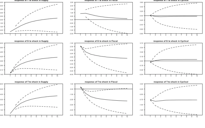
forecast error variance decomposition. 22 We have summarised all results in Figures 3a and

3b. This prepares the ground for an analysis of the fiscal indicator in section 4.3.

The effect of productivity shocks is to lift up real output permanently (Figure 3a). The speed

of accumulation is rather fast: after five years, the major part of the shock has worked out. In

Germany, this happens even faster. The sampling uncertainty around the effect is large, but

given the large bounds we have used, the significance of most impulse responses after

some years is actually surprising. To what extent are these supply shocks driven by fiscal

developments? In France and Portugal, these shocks go hand in hand with positive

long-term effects on total expenditures and revenues as well. This effect is also strongly

significant.23 The difference between revenues and spending responses is not significant,

hence it is not obvious that this leads to a build up of public debt. In Germany and Spain on

the contrary, revenues do not change significantly, but government expenditures shrink

considerably, leading to large accumulated surpluses at a horizon of 10 years.

But whether the causality runs from fiscal policy to productivity growth, or vice versa, is not

obvious. Recall that the supply shock contains productivity shocks that may emanate from

the private as well as the public sector. The significant co-movement of spending and

revenues suggests that fiscal ‘supply’ shocks are an important source of the overall

productivity shock.24 If these relations are positive (the case of France and Portugal), this

implies higher spending or tax revenues have contributed to economic growth. In the

opposite case (Germany or Spain), a reduction of spending – and less so a lower tax burden

– would trigger higher potential output growth. But there are a few alternative explanations.

Positive economic shocks that enlarge the tax base would – for a given tax rate –

automatically lead to a larger revenue intake owing to automatic stabilisers. For reasons of

political economy, this could lead the government to directly spend the proceeds of the

treasury. This expansion of the budget could consequently get locked in and lead to a

22 _{Impulse responses follow a one standard shock, and are plotted over a 10 year horizon with 90% confidence}

intervals, based on a bootstrap with 5000 draws.

23 _{As the long-term elasticity of both spending and revenues is larger than unity, this looks like a ‘Wagner’ style}

government expansion owing to economic growth.

24 _{We considered the effect of loosening the long-term constraint on either government expenditures or revenues}

19

permanent rise in government expenditure. This mechanism would work for both permanent

and cyclical shocks, if we assume that the government does not systematically react in

different ways to permanent or transitory economic shocks. This allows us to get some

insight in the importance of the private versus public productivity shocks. The fiscal

responses to cyclical shocks, which include business cycle shocks with transitory output

effects that are not related to fiscal policy can give some indication. Surprisingly, the effects

of cyclical shocks on output are hardly significant and indicate the small size of temporary

economic fluctuations.25 As a consequence, there is not always an obvious simultaneous

rise in tax revenues. In Germany and Portugal, government revenues do rise in response to

a positive output gap, and this effect remains permanent. Moreover, in both countries

government expenditures tend to rise as well. This gives some support for the ‘ratcheting up’

effect on spending. In France or Spain instead, government spending does not react in a

significant way and tax revenues even tend to decline.

If we consider in some more detail the two countries in which catching-up phenomena may

be expected to be important, we cannot clearly distinguish between the two alternative

explanations. Both in Spain and Portugal is the reaction of fiscal variables to temporary and

permanent shocks similar. This downplays the importance of productive fiscal policy

contributing to economic growth. A comparison of the impulse responses shows that only a

minor effect would be left in the case of Portugal. Evidence on Spanish public finances

presents a slightly different picture. Positive supply shocks are accompanied by a strong

decrease in total spending, and this effect is much more pronounced than the reduction in

spending after a cyclical shock.

In France and Germany instead, the reaction of fiscal variables to permanent shocks is

opposite to the reaction to business cycle shocks and supports the view that fiscal variables

driving long-term growth in both countries. That spending and revenues go up after a

positive supply shock, whereas there is a non-significant response or a decline following

cyclical shocks, would suggest a larger role for productive public spending in France instead.

Evidence for Germany rather seems to indicate a too large size of government. We find that

revenues and spending go up permanently after cyclical shocks, but positive supply shocks

tend to be associated with reductions in spending.

[INSERT FIGURE 3a HERE]

20

The fiscal shock then regards all discretionary policy interventions on spending and/or

revenues that are not systematically related to the cycle and have only temporary effects on

the economy. These discretionary fiscal shocks have somewhat prolonged effects on output.

There is a lot of uncertainty around this effect and none of the responses is really significant.

We scale the impulse responses in Figure 3a such that they always display positive output

effects. We do not find the typical result of small positive Keynesian effects on output in all

countries. In Germany and Spain, a typical Keynesian response would follow upon demand

boosting deficits. In France and Portugal on the other hand, fiscal contractions would lead to

positive short-term effects on output instead. Such different responses likely depend on the

composition of the fiscal adjustment or other structural parameters in the respective

economies, but cannot be further examined in the current model.

The different responses of spending and revenues to both economic shocks might indicate a

delicate issue in the identification of policy. If fiscal policy reacts in a systematic way to

economic shocks by changing its discretionary use of spending and/or revenues, this

simultaneity blurs the distinction between the economic and the fiscal shock. This might be

the case in France and Spain where tax revenues decrease after positive temporary output

shocks, for example. But another indication is given by the rise in spending in economic

booms in Germany or Portugal. It indicates policies that react in a discretionary way so as to

repeal the use of automatic stabilisers. The fiscal indicator captures these policy biases. Our

discussion will show how important this policy bias is for understanding fiscal trends in EU

countries.

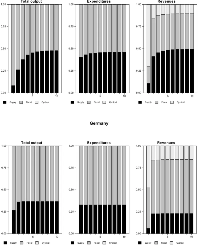
What does this imply for the contribution of fiscal policies to output variation (Figure 3b)?

Supply shocks account for at least 50% of total variance in output at all horizons, and this

goes up to 90% in Portugal and Spain. For the latter countries, this was perhaps to be

expected given their strong economic growth over the last two decades. Most of the

variation in output is thus caused by productivity shocks even at short horizons. As we do

not separately identify private and public supply shocks, we cannot really quantify the

relative magnitude of both channels. But as pointed out above, we think that productive

spending or revenues has contributed to some extent to the variance of output. The demand

effects of fiscal policy in France and Germany are at least as large as those of supply

effects. In Portugal or Spain instead, only a minor role is played by discretionary fiscal policy.

The contribution of cyclical fluctuations to variations in output is negligible, as was to be

21

What factors can account for these results? The large role played by fiscal policy in

explaining output variation is not inconsistent with previous findings in the literature for large

EU countries (De Arcangelis and Lamartina, 2004), but seems on the higher side of the

range usually found. If we take the result at face value, it would suggest that the temporary

demand effects of fiscal policy are probably much larger than the supply effects in the

long-term. This would imply that both RBC and New Keynesian models are missing some

aspects of fiscal transmission. But as we cannot precisely quantify the importance of the

latter shocks, we would not want to claim validation of any of the theoretical models with our

approach. This result nevertheless reveals that models of fiscal policy need to attribute

important roles to both demand and supply side effects.

We think that the reason for the large contribution of fiscal policy is to be found elsewhere.

To the extent that automatic stabilisers reduce the volatility of economic fluctuations, the

tendency of governments to reduce taxation and/or rise spending in a procyclical way only

adds to short-term output fluctuations and brings about aggregate macroeconomic

instability. This policy volatility can moreover have negative effects on the long-term growth

prospects of the economy.26 The unwinding of previous taxation decisions goes against the

principle of ‘tax smoothing’. The procyclicality of budgets implies negative supply-side

effects. This explains the surprisingly low contribution of cyclical fluctuations.

[INSERT FIGURE 3b HERE]

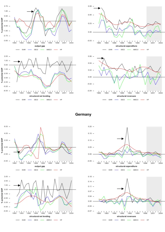
Before going deeper into the past trends in fiscal policy, we want to check our model on

some other aspects too. We compute the output gap based on the historical decomposition

of the output series as actual minus potential output (y-

y

*). In Figure 4 (top left panel),27 _we

have repeated for comparison the output gaps of the European Commission, OECD and the

one obtained by applying a Hodrick-Prescott filter. There is a rather close correspondence

between these measures and our supply shock based gap for France and Germany. Given

that we have used the OECD elasticities only for distinguishing shocks with transitory effects

on output, this is all the more remarkable. The smooth gap for Portugal and Spain underlines

the importance of supply relative to demand shocks in both countries. This might indeed be

expected given the strong economic catch-up that both countries have experienced. We

believe that potential output tracked much closer actual output developments in these

26 _{We are certainly not the first study to document that European countries have not left automatic stabilisers to}

work, but instead have overturned these in a procyclical way. We do show however the macroeconomic instability that results as a consequence. With other models, Alesina and Bayoumi (1996) showed how fiscal policy at the US state level rather contributes to macroeconomic instability, and how fiscal rules have been useful in constraining discretion. Similar cross-country evidence is provided by Fatás and Mihov (2003b).

22

countries. The usual statistical filtering methods are not adequate to capture this trend

behaviour over small samples. Cyclical fluctuations are therefore rather minor. We provide

some further robustness checks in the Appendix 2.28

Overall, in all countries, there definitely was an improvement in economic conditions at the

start of EMU. We find that economic conditions have worsened in both France and Germany

in recent years. We nevertheless find the crisis in Germany to have set in somewhat earlier

and to be more prolonged. As cyclical fluctuations are not large, we do not find much

economic slack in recent years in Spain or Portugal.

[INSERT FIGURE 4 HERE]

4.3. The fiscal indicator

We are now ready to discuss the indicator of discretionary fiscal stance. In general, the

measure is more volatile than the measures derived with conventional methods (see Figure

4, bottom left panel). In many instances, our measure leads the smoothed measures in the

direction of change. The fiscal indicator is usually smaller than the cyclically adjusted deficit.

This reflects the definition of the structural balance, by which we take out the automatic

stabilisers and the induced stabilisation effects caused by fiscal policies. In addition, fiscal

policy also affects permanent output and therefore the structural fiscal position fluctuates

around balance.

The indicator is also much more volatile. This follows from the major contribution of supply

and fiscal shocks to the variation in output, spending and revenues (Figure 3b). As we

discuss below, one of the causes of this strong volatility – apart from the dominant supply

side shocks – is the procyclical bias that characterises fiscal policymaking that induces extra

variation, especially so in government revenues.

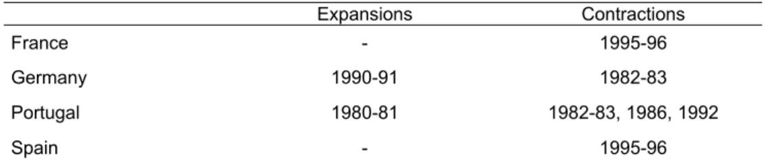
We may then expect our fiscal measure to coincide with some episodes of fiscal laxness or

retrenchment. We consider the budget to undergo a strong expansion (contraction) when the

cyclically adjusted primary balance falls (increases) by at least 2 percentage points of GDP

in one year, or at least 1.5 percentage points on average in the last two years. This is the

28 _{A rough indication on the robustness of our output gap measure can also be given by the dates of peak and}

23

measure proposed by Alesina and Ardagna (1998). In Table 5, we gather those fiscal years

in which a strong expansion or adjustment has occurred in our dataset (see Afonso, 2006).

At first sight, the correspondence is rather close. Comparing the changes in Figure 4 (bottom

left panel) to the years in Table 5, we detect all events that the Alesina-Ardagna measure

also suggests. For example, we find budgetary cost of Reunification on German public

finances to have been large. The Maastricht rules have also led to considerable fiscal

retrenchment in France and Spain. There are a few events in Portuguese fiscal policy over

the eighties that we do not date exactly. But we do find a switch between contraction and

expansion starting in 1982-83. The Alesina-Ardagna measure does not pick up all

expansions and contractions that we find, however. Some of these episodes correspond to

well known changes in the fiscal stance (e.g. the ‘Mitterand’ budgets in France 1981).

Another major expansion in France in 1992 follows upon a string of expansionary budgets.

Spain equally undergoes major expansions in the early eighties and nineties (1981 and 1993

respectively). Fiscal policy is also lax in Portugal (1990). Prolonged contractions occur over

the eighties in France, Germany and Spain too.

Table 5. Large fiscal expansions and contractions

Expansions Contractions

France - 1995-96

Germany 1990-91 1982-83

Portugal 1980-81 1982-83, 1986, 1992

Spain - 1995-96

Source: adapted from Afonso (2006), following the measure used by Alesina and Ardagna (1998).

Concentrating on the period just before EMU, we can see a substantial shift in discretionary

policies towards structurally positive net lending ratios. This is perhaps least visible in

Germany, but the initial conditions were probably not such as to urge a strong and prolonged

consolidation for reaching the Maastricht deficit limit. A substantial consolidation had already

taken place at the end of the eighties. In the other countries, the structural effort was more

drawn out. France started consolidation already in 1993, while it gathered pace in Portugal

and Spain only in 1995. This also confirms evidence in Fatás and Mihov (2003a).

How has this consolidation been achieved? The right hand side panels of Figure 4 plot the

growth rates of structural expenditures and revenues. These reveal that structural

consolidations in the nineties have been based on a mixture of expenditure and revenue

measures. But the combination of adjustments in the policy instruments has changed over

24

expenditure growth and in some cases even relevant spending cuts (Germany and

Portugal). This strategy is reversed closer to the deadline of EMU. Tax increases start to

bear the largest burden for bringing down deficits. Given the urgency of qualifying for the

EMU criteria, taxes have seemingly been the easiest instrument to adjust. Notice the rather

close match between the VAR-measure of structural spending and revenues and the

(difference log of the) HP-trend on unadjusted total expenditure and revenues. The

measures of OECD and AMECO display slightly lower growth rates. This owes again to our

definition of the structural series. The efforts in reaching EMU led to the levelling off or even

moderate declines in debt ratios. A plot of the structural fiscal indicator to the debt ratio

shows how well the indicator captures these consolidations in debt (Appendix 2).

What went wrong then with the application of the Stability and Growth Pact in France,

Germany and Portugal upon entry in EMU? The causes are again rather similar across

countries. The increased tax revenues in the years prior to EMU led to a starting point of

structural surplus. The persistence in these tax rises improved actual balances thanks to the

favourable economic conditions at the time. But this has been exploited to increase

expenditures in a commensurate way. Especially in Portugal, the expansion in expenditures

seems to have held back an improvement in the structural position. The only exception here

is Spain that further brought down expenditure, even in the presence of strong revenue

increases. Simultaneously, the tax revenues that stream in during economic boom seem to

have been undone by decisions to bring down tax rates in most countries. This considerably

worsened the structural balance. As economic boom turned into bust again, the decline in

revenues led to a substantial worsening of actual balances, pushing the deficit beyond the

3% threshold. However, the revenue declines have hardly ever been matched by sufficient

cutbacks in government spending in the following years. Corrective measures in 2004 have

improved the structural deficit. But the measures are mainly taken on the revenue side

again, by undoing once more previous decisions to cut tax rates. To avoid further

infringement of the budget rules, the adjustment in Germany and France has taken place via

the route of tax rises during economic slack. This has once more reinforced the procyclical

bias in fiscal policy-making. This also highlights the mechanism by which spending gets

locked in, and causes a ‘ratcheting up’ in the size of government.

The overall situation seems less dramatic in Portugal, as revenue changes have been

supported by equivalent spending decisions.29 For Spain, the moderate decline in tax

29 _{One should notice that several one-off measures mask the true deterioration in the Portuguese or the Spanish}

25

revenues in 2001 and 2002 was not entirely matched with spending cuts, leading to a slight

deterioration of the structural indicator. The expansionary measures taken in 2004 have led

to a breach of a balanced structural budget for the first time since 1995. Unsurprisingly, the

expansion of fiscal policies in all countries reflects itself in rising debt ratios in recent years

(see Appendix 2).

How useful is our indicator for assessing budgetary reform? We have argued above that

aggregate spending or revenue measures contribute to long-term growth. Its contribution

may perhaps be small relative to productivity rises in the private sector, and part of the effect

could be swamped due to procyclical policies that induce macroeconomic fluctuations (and

its consequent negative effects on growth). We do not believe this is the final word on the

contribution of fiscal policy. A more detailed analysis of different spending/tax items could

shed light on their specific growth enhancing effects.

4.4. Some sensitivity analysis

The results might be influenced by some particular parameter value that we have drawn

from the OECD (Girouard and André, 2005) in order to distinguish business cycle and fiscal

demand shocks. There are various reasons for considering these aggregate elasticities with

some caution.

First, elasticities are assumed to be time-invariant. These are not representative of the tax

and spending structures that have prevailed in historical samples, however. In some

countries, the expansion of the welfare state has led to gradually larger tax bases and

dramatic changes in tax systems (Portugal and Spain). But even in France and Germany,

time-variation cannot be neglected. Budget elasticities tend to move over the business cycle

as well (Bouthevillain et al., 2001). Changes in elasticities also throw up a more subtle

difficulty in the interpretation of the fiscal shocks that we have already discussed in section

4.2. On the revenue side, discrete policy changes involve decisions on the ratio of average

to marginal tax rates and the breadth of tax bases rather than on total amounts.30 Only if

changes in total revenue amounts coincide with these decisions, do we identify correctly

shocks on the revenue side of the budget. Second, given the difficulties in identifying all

channels through which changes in interest rates and inflation may impinge on various

revenues and spending categories, the OECD simply abstains from adjusting interest