Engineering
ISSN: 1809-4430 (on-line)
_________________________
2 Universidade Federal de Santa Maria/Santa Maria - RS, Brasil. 3 Universidade Federal de Santa Catarina/Curtibanos - SC, Brasil. 4 Geocamp Topografia Ltda./Passo Fundo - RS, Brasil.
TECHNICAL PAPER
QUALITY OF A DIGITAL TERRAIN MODEL FOR SANTA CATARINA STATE
Doi:http://dx.doi.org/10.1590/1809-4430-Eng.Agric.v36n6p1261-1271/2016
ALEXANDRE TEN CATEN1*, RICARDO S. D. DALMOLIN2, EVANDRO L. BOEING3,
FERNANDO A. VITALIS4, WALQUÍRIA C. DA SILVA3
1*Corresponding author. Universidade Federal de Santa Catarina/ Curitibanos - SC, Brasil. E-mail: [email protected]
ABSTRACT: Relief characterization using a digital terrain model (DTM) is widely applied in erosion, soil and vegetation modeling. However, factors, such as acquisition technology and the spatial resolution of the digital model, affect modeling results. The aim of this study was to characterize noises in a DTM of the entire state of Santa Catarina recently made available through
the state’s Sustainable Economic Development Secretary and to evaluate different methods of interpolation and smoothing of the original 1 m resolution to a new digital model with a spatial resolution of 15 m. Using the SAGA GIS program, spurious data that appeared as peaks and sinks were removed from the digital model. Of five processing procedures, the following three were used for smoothing: a Gaussian filter, a Lee filter, and mesh denoising. The remaining two were for interpolation: nearest-neighbor, and ordinary kriging. Altimetric reference data were collected in the study area of 11,597 km² with two dual-frequency GPS RTK receivers located in the Celso Ramos community in the municipality of Frei Rogério (SC). The root mean square error showed that the documented values of the aerial survey report were consistent with the findings of this study. However, the GPS RTK data showed a difference of 1.07 m compared with the original DTM with 1 m spatial resolution. There were pixels with peaks and sinks in the digital model of the Santa Catarina State.
KEYWORDS: digital elevation model, geomorphometry, slope, digital soil mapping, aerial imagery.
INTRODUCTION
The processing of a digital terrain model (DTM) that applies geomorphometrics (HENGL & REUTER, 2008) in a geographic information system (GIS) facilitates the generation of primary (e.g., slope and aspect) and secondary (e.g., profile and planar curvatures) topographic attributes. Studies have shown the potential of topographic attributes for environmental modeling (MINELLA & MERTEN, 2012), land cover identification (LAMPARELLI et al., 2011) and soil class and properties prediction (TEN CATEN et al., 2011; SAMUEL-ROSA et al., 2013). However, the value assumed by a topographic attribute is a function of the selected algorithm for DTM processing (KOPECKÝ & ČÍŽKOVÁ, 2010). In addition, the various topographic attributes are affected by the spatial resolution of the DTM used to generate them (SØRENSEN & SEIBERT, 2007) and by the DTM production source (GUEDES & SILVA et al., 2012).
Spatial resolution and the DTM data source have a substantial impact on derived topographic attributes and their subsequent application (ZHANG et al., 2008). A study by KIENZLE (2004) demonstrated that a DTM derived from a small landscape sampling density has limited application to environmental and hydrologic modeling. The same author also showed that terrain attributes, such as elevation, slope and the planar and profile curvatures, exhibit significant variation at different spatial resolutions. According to author, slope is not well characterized by a DTM with a spatial resolution smaller than 25 m, and profile curvature values are underestimated in a DTM of lower spatial resolution. Furthermore, the importance of using a DTM with a spatial resolution of at least 20 m increases from a primary to a secondary and finally to a compound topographic attribute. For applications related to crop-harvesting maps, ERSKINE et al. (2007), in a study with relief amplitudes up to 21 m, recommend applying a pixel size of 30 m. However, the authors stress that the pixel size is a function of the DTM’s application.
In a study by ZHANG et al. (2008), the application of a DTM produced by LIDAR with a spatial resolution of 10 m facilitated a positive association between data volume and predictive power in sediment-yield modeling in two watersheds of 110 and 176 hectares. These authors also showed that data obtained using a LIDAR technique, with a resolution of 30 m, produced unsatisfactory results. The authors also confirmed that SRTM data interpolated to 30 m are ineffective in modeling sediment yield.
In 2009, the Secretary of State for Economic and Sustainable Development (SDS) of Santa Catarina State through held a public bidding to hire an aerial survey service. Among the data collected at that time was a DTM available in a spatial resolution of 1 m for the entire state, a total of 97,037 square kilometers (SDS, 2012). In this context, the objective of this study was to conduct a quality check of the data in this DTM and to evaluate procedures for the interpolation and smoothing of the original DTM to a new spatial resolution of 15 m.
MATERIAL AND METHODS
The area selected for the study is located in the Celso Ramos community of the municipality of Frei Rogério. Frei Rogério is in the Serrana region of Santa Catarina, near the state center (Figure 1). The DTM for this study has an area of 11.597 km², with a spatial resolution of 1 m. The relief of the study area is characterized by gentle rolling hills, with an elevation that ranges between 810 and 945 m.
FIGURE 1. Location of the study area in Brazil and Santa Catarina. Dashed lines indicate the position of the drainage system. Solid lines indicate contour lines with elevation values in meters. White dots indicate the 70 points used to verify the DTM with GPS RTK. Coordinates in UTM projection zone 22 / SIRGAS 2000.
Five procedures for DTM processing were evaluated. The following three procedures were used for smoothing: a Gaussian filter (BÖHNER et al., 2014), a Lee filter (LEE, 1980), and mesh smoothing (STEVENSON et al., 2010). The remaining two procedures were used for interpolation: nearest-neighbor, and ordinary kriging (WALTER et al., 2001). The kriging was performed using Vesper 1.6 software (WALTER et al., 2001). The other four procedures were performed using SAGA GIS 2.1.0. All analyzed DTMs had spatial resolutions of 15 m. This value was selected based on results previously discussed in ZHANG et al. (2008) and KIENZLE (2004). That is, this spatial resolution was deemed an appropriate value for future studies, because it does not require processing an excess of data in a DTM of higher spatial resolution (<15 m), or cause information in a DTM with much lower resolution (30 or 60 m) to be lost.
exponential, with a nugget effect of 36.21 m, a sill of 1996.2 m and a range of 2692.5 m. The variation in the data was defined by Vesper 1.6 as isotropic.
To quantitatively compare the variations in the landscape and how they were represented in each DTM of 1 and 15 m, a field campaign was performed to collect the elevation of 70 points in the study area. The elevations were collected using two GPS instruments (Topcon Hiper GGD; model Lite Plus) with dual-frequency receivers in a real-time kinematic (RTK) configuration. The application of GPS RTK has proven effective as a fast, precise method to collect reference data for studies that investigate terrain elevation (FARAH et al., 2008; KIZIL & TISOR, 2011). One GPS unit (termed Base) was installed near the center of the study area, and the other (termed Rover) was carried throughout the study area to a maximum distance of 2 km from the Base. The elevation of the Base receiver was determined as being the same as that of the corresponding pixel in the original 1 m DTM. Thus, considering the small size of the study area, the ellipsoidal GPS elevation could be used as reference to characterize the local relief. In the RTK mode, the GPS Rover was set to collect latitude, longitude and elevation using the fixed solution of ambiguities, with a collection of three epochs in each of the sampled points.
The elevation data collected in the field campaign were tabulated for the quantitative analysis of the DTM. Each of the five procedures tested was assessed by comparing the descriptive statistics of (i) the elevation values of the different DTMs, (ii) the differences between the original DTM and the DTM of 15 m resolution, and (iii) the differences between the elevation according to GPS RTK and each DTM. The descriptive statistical parameters were minimum, maximum, mean, standard deviation, root of the mean square error (RMSE), skewness and kurtosis. The statistical data processing was performed using the R programming language (R DEVELOPMENT CORE TEAM, 2014).
RESULTS AND DISCUSSION Noise in the DTM
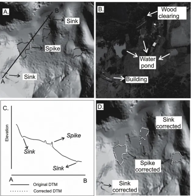
The observation of the data contained in the original 1 m DTM enables the visualization of the noise that is present in the form of spikes and depressions (Figure 2A). It can be observed in Figure 2B that noise in the form of peaks is linked to the edges of ponds. Additionally, noise in the form of depressions is linked to abrupt differences between the digital surface model (DSM) and the derived DTM (Figures 2A and 2B). The DSM is a mathematical representation of the three-dimensional spatial distribution of the physical surface variations on Earth and describes the topography together with all aboveground elements, such as trees and buildings (SDS, 2012).
According to the aerial survey report, the DSM was generated by an automatic measurement technique from correspondence points between aerial stereo pairs using a technique known as epipolar geometry (SDS, 2012). This digital correlation technique reduces the search space for corresponding points on adjacent images in epipolar lines. In turn, these lines are calculated based on image geometry and orientation in the object space. After the creation of the DSM, the DTM extraction was performed according to the following procedure: i) visual inspection of DTM features (e.g., buildings and vegetation), ii) creation of filtering masks, iii) application of masks to remove and smooth points in the DTM, and iv) replacement of eliminated / smoothed points by measured points. Then, the DTM was generated in the form of a triangulated irregular network (TIN) using Inpho software (SDS 2012).
further investigations should be conducted to improve the understanding of the origins of such noise, particularly in other regions of the DTM of Santa Catarina State with its total of 97,037 km².
FIGURE 2. Presence of spurious data in the form of spikes and sinks: (A) the location of noise in a DTM extract; the continuous line represents a transect 'a-b' for analysis in (C); (B) causes of spurious data in (A); (C) schematic representation of a transect 'a-b' DTM before and after correction; (D) DTM corrected by removing the effects of spikes and sinks.
Visual analysis of Figures 2C and 2D reveals the effect of applying the spurious-data correction techniques used in this study. The DTM Filter algorithm of SAGA GIS 2.1.0 facilitated the identification of a pixel surrounded by other pixels of much lower values and its elimination from the DTM. This technique is based on VOSSELMAN (2000), who states that it is unlikely that an abrupt change in elevation between two neighboring pixels is due to the presence of a cliff or steep slopes. Similarly, a pixel completely surrounded by a group of much higher pixel values was corrected using the Fill Sinks algorithm. This technique not only fills the depressions but also preserves the flow direction between pixels toward smaller elevations. Thus, a minimum relief gradient is maintained between the pixels when the Fill Sinks algorithm is applied (WANG & LIU, 2006).
hydrologically consistent so it can be used in modeling phenomena that depend on water movement through the landscape, such as in wetlands, oxidation and reduction zones as well as removal and deposition spots.
Quantitative analysis of the DTM used in the study
In this study, five procedures were applied to evaluate the effects of disintegrating (i.e., downscaling) the original DTM with a spatial resolution of 1 m into a coarser one of 15 m (Table 1). The descriptive statistics of the original DTM and the five generated DTMs reveal that the models share similar characteristics, such as the lowest and highest points represented in each of the relief models. The range between the lowest and highest points ranged from 171.02 m in the DTM generated using the Lee filter to 171.52 m in the original DTM. The data distribution statistics indicated that all digital models for the study area have a symmetrical distribution of elevation values close to the normal, with a moderate value from 0.52 to 0.54 for asymmetry. Regarding the shape of the distribution, the kurtosis values (between 0.52 and 0.54) indicated that the elevation values in the study area are close to the normal distribution, with a curve with mesokurtic characteristics (the values are not included in Table 1).
The comparison between the original DTM and each of the five generated DTMs reveals slight differences between these relief models (Table 1). The largest differences can be observed in the nearest-neighbor DTM, which reach a range of 16.45 m. This interpolation procedure does not evaluate surrounding pixels and only samples (for the new DTM of 15 m) the closest pixel value in the DTM of 1 m. Therefore, in certain locations, the nearest-neighbor procedure highlights the differences between the DTMs. However, the lower amplitude differences between the resampled and the original DTMs are apparent in the Gaussian filter procedure, with a value of 13.62 m, and exhibited a smaller standard deviation of 1.25 m. This procedure applies a smoothing operator in a window of 3 x 3 pixels. Thus, the pixel value in the new DTM is an average value that is contextualized from the values of neighboring pixels.
TABLE 1. Descriptive statistics for the analyzed DTM (values in meters).
Statistics for the original 1 m DTM and the five procedures used in the study
DTM Minimum Mean Maximum Range Standard deviation
Original1 805.07 868.48 976.59 171.52 31.25
NearNei2 805.07 868.70 976.58 171.51 31.28
LeeFilter2 805.10 868.61 976.12 171.02 31.20
MeshSmo2 805.08 868.70 976.50 171.42 31.24
GausFilter2 805.14 868.70 976.27 171.13 31.18
OrdKrig2 805.08 868.47 976.24 171.16 31.12
Statistics for the differences between the original 1 m DTM and each other DTM (15 m)
DTM Minimum Mean Maximum Range Standard deviation
NearNei -9.29 0.22 7.16 16.45 1.21
LeeFilter -9.29 0.13 6.87 16.16 1.22
MeshSmo -7.58 0.22 6.86 14.44 1.36
GausFilter -6.48 0.22 7.14 13.62 1.25
OrdKrig -9.15 -0.01 6.93 16.08 1.53
Statistics for the differences between the elevation obtained by GPS RTK and each DTM
DTM Minimum Mean Maximum Range Standard deviation RMSE
Original -4.95 0.05 3.51 8.46 1.08 1.07
NearNei -6.20 0.09 3.38 9.58 1.42 1.41
LeeFilter -5.30 -0.24 3.20 8.51 1.55 1.56
MeshSmo -5.81 0.06 3.24 9.06 1.44 1.43
GausFilter -5.33 0.05 3.33 8.67 1.45 1.44
OrdKrig -4.55 -0.24 3.53 8.09 1.68 1.68
The observation of standard deviation values (Table 1) in the five DTMs varied between 1.21 and 1.53 m for the nearest-neighbor and kriging methods, respectively. Associated with the values discussed in the previous paragraph, these numbers indicate that the methods of interpolation and smoothing generally reproduced the information contained in the original 1 m DTM. However, occasional punctual differences of a few meters occurred.
The differences between the GPS RTK data and the original DTM ranged from -4.95 to 3.51 m, with an amplitude of 8.46 m (Table 1). The standard deviation of the differences between these two data sets was 1.08 m, and the RMSE was 1.07 m. These data are consistent with the results of the aerophotogrammetric flight report (SDS, 2012). However, the report does not mention the occurrence of punctual discrepancies in the original 1 m DTM or their origin, as indicated by data obtained using GPS RTK and in the DTM. In ERSKINE et al. (2007), in areas of up to 70 hectares with differences in elevation of 21 m, the authors concluded that due to the technique used for their generation the DTM errors are more significant than the interpolation procedure or the pixel size. Thus, this area is one in which future studies can increase our understanding of the effects of the techniques used to generate the SDS (2012) DTM.
Among the evaluated DTMs, the largest differences in standard deviation and RMSE observed in ordinary kriging were 1.68 and 1.68 m, respectively. ERDOGAN (2009) concluded that the magnitude and distribution of errors in the interpolated DTM were associated with relief characteristics, sampling density and the applied interpolation algorithm. An interpolation of 24,000 points, which was obtained by conventional leveling, ordinary kriging and cross validation, indicated RMSE values of 0.41 and 0.80 m for spatial resolutions of 10 and 20 m, respectively. For this author, ordinary kriging represents a disadvantage because of the time required to process large volumes of data. The efficiency of ordinary kriging is significantly more related to the quality of spatial variability modeling, which uses semivariogram adjustment, than the kriging method itself.
The nearest-neighbor interpolation method generated a DTM with elevation values that were more similar to the local relief, which is indicated by the RMSE value of 1.41 m. This method simply sets the value of the new pixel (based on the original pixel value) closer to the center of this new spatial resolution. The adoption of the nearest-neighbor interpolation results in a fast approach but with a lower reproductive capacity with respect to the original DTM compared with the bilinear interpolation techniques and cubic convolution (WU et al., 2008).
Spatial distribution of the differences between GPS RTK and the studied DTM
FIGURE 3. Spatial distribution of the differences between elevation values collected by GPS RTK and the five resampled DTMs: (A) original, (B) nearest neighbor, (C) Lee filter, (D) mesh smoothing, (E) Gaussian filter (F) ordinary kriging.
As previously described, to generate the DTM from the DSM, a number of steps were applied to extract the influence of aboveground elements (e.g., trees and buildings). Figure 1 shows that the study area has many elements, such as trees, buildings and water ponds located in Region C of Figure 3A. The presence of these elements in the DSM influences the quality of the resulting elevation in the DTM. Region C of the study area has the largest number of discrepancies between the DTM and the field-collected data (Figures 3A to 3F). Therefore, in future proposals to assess and mitigate the noise in the SDS (2012) DTM, special attention should be paid to areas that present aboveground elements, such as forests and urban centers.
In future studies, quality verifications of the data presented in the SDS (2012) DTM, which is available for the entire state of Santa Catarina, should be expanded. It is important that these data in different spatial resolutions are implemented and evaluated as a basis for the derivation of primary, secondary and compound topographic attributes. The applicability of these attributes should be considered, for example, in environmental modeling, the prediction of soil properties, sediment production and with respect to the distribution of fauna and flora. It is also important to analyze the magnitude of uncertainties generated during environmental modeling due to the presence of errors in the DTM. Error propagation possibly due to noise in the SDS (2012) DTM should also be examined.
CONCLUSIONS
Noise in the form of sinks and spikes occurs in the DTM with a spatial resolution of 1 m in the study area. Data collected in a field campaign using GPS RTK technology indicated a RMSE of 1.07 m in the DTM available for the tested area.
Among the interpolation procedures, the nearest-neighbor approach generated a 15 m DTM with elevation values closer to those obtained in the field (RMSE of 1.41 m). Interpolation using ordinary kriging generated a DTM with the largest differences in relation to the data collected in the field (RMSE of 1.68 m) and demanded a longer processing time. Interpolation using a Gaussian filter, a Lee filter and mesh smoothing did not generate smaller RMSE values than the DTM interpolated using the nearest-neighbor method.
ACKNOWLEDGMENTS
We would like to thank CNPq for providing a scholarship and funding to perform this research through process nº550177/2012-4. In addition, funds were allocated by process nº442718/2014-4 MCTI/CNPq/Universal14/2014. We would like to thank the anonymous reviewers for their suggestions and comments.
REFERENCES
BARBOSA, A. P.; SILVA, A. F. DA.; ZIMBACK, C. R. L. Modelo numérico do terreno obtido por diferentes métodos em cartas planialtimétricas. Revista Brasileira de Engenharia Agrícola e Ambiental, Campina Grande, v.16, n.6, p.655–660, 2012. Disponível em: <
http://www.scielo.br/pdf/rbeaa/v16n6/v16n06a10.pdf>. Acesso em: 20 ago. 2014.
BÖHNER, J.; BOCK, M.; HASELEIN, F.; CONRAD, O.; KÖHTE, R.; RINGELER, A.; SELIGE, T. Digital Soil Mapping in SAGA GIS. SAGA User Group. Göttingen. 2014. Disponível em: <http://eusoils.jrc.ec.europa.eu/esdb_archive/ESBN/Esbn_Zagreb/Presentations/DSM/DSM_SAGA _Ringeler.pdf>. Acesso em: 20 ago. 2014.
CHAGAS, C. S.; FERNANDES FILHO, E. I.; ROCHA, M. F.; CARVALHO JÚNIOR, W. DE.; SOUZA NETO, N. C, Avaliação de modelos digitais de elevação para aplicação em um
mapeamento digital de solos. Revista Brasileira de Engenharia Agrícola e Ambiental, Campina Grande, v.14, n.2, p.218-26, fev. 2010.
EGELS, Y.; KASSER, M. Digital photogrammetry. New York: Taylor & Francis, 2001. 368p.
ERDOGAN, S. A comparison of interpolation methods for producing digital elevation models at the field scale. Earth Surface Processes and Landforms, Malden, v.34, n.3, p.366-76, mar. 2009. ERSKINE, R.H. GREEN, T.R.; RAMIREZ, J.A.; MCDONALD, L.H. Digital elevation accuracy and grid cell size: effects on estimated terrain attributes. Soil Science Society of America Journal, Madison,v.71, n.4, p.1371-1380, 2007.
GUEDES, H. A. S.; SILVA, D. D. DA. Comparison between hydrographically conditioned digital elevation models in the morphometric characterization of watersheds. Engenharia
Agrícola, Jaboticabal, v. 32, n. 5, p. 932-43, out. 2012.
HENGL, T.; REUTER, H. I. Geomorphometry: concepts, software, applications. Developments
in soil science. Amsterdam: Elsevier, 2008. 772p.
KIENZLE, S. The effect of DEM raster resolution on first order, second order and compound terrain derivatives. Transactions in GIS, Malden, v.8, n.1, p.83-111, jan. 2004.
KIZIL, U.; TISOR, L. Evaluation of RTK-GPS and total station for applications in land surveying. Journal of Earth System Science, Delhi, v.120, n.2, p.215-21, abr. 2011.
KOPECKÝ, M.; ČÍŽKOVÁ, S. Using topographic wetness index in vegetation ecology: does the algorithm matter? Applied Vegetation Science, Edinburgh, v.13, n.4, p.450-459, 2010.
LAMPARELLI, R. A. C.; NERY, L.; ROCHA, J. V. Utilização da técnica por componentes principais (ACP) e fator de iluminação, no mapeamento da cultura do café em relevo montanhoso. Engenharia Agrícola, Jaboticabal, v. 31, n. 3, p. 584-97, jun. 2011.
LEE, J. S. Digital image enhancement and noise filtering by use of local statistics. IEEE
Transactions on Pattern Analysis and Machine Intelligence, Los Alamitos, v.2, n.2, p.165-68, mar. 1980.
MINELLA, J. P. G.; MERTEN, G. H. Índices topográficos aplicados à modelagem agrícola e ambiental. Ciência Rural, Santa Maria, v.42, n.9, p.1575-82, set. 2012.
PINHEIRO, H. S. K.; CHAGAS, C. DA S.; CARVALHO JÚNIOR, W. DE.; ANJOS, L. H. C. DOS. Modelos de elevação para obtenção de atributos topográficos utilizados em mapeamento digital de solos.Pesquisa Agropecuária Brasileira, Brasília, DF, v.47, n.9, p.1384-1394, 2012. R DEVELOPMENT CORE TEAM. R: A language and environment for statistical computing. R foundation for statistical computing. Vienna. 2014. Disponível em: <http://www.r-project.org.> Acesso em: 20 ago. 2014.
SAMUEL-ROSA, A.; DALMOLIN, R. S. D.; MIGUEL, P. Building predictive models of soil particle-size distribution. Revista Brasileira de Ciência do Solo, Viçosa, MG, v.37, n.2, p.422-30, mar./abr. 2013.
SDS – Secretaria de Desenvolvimento Econômico e Sustentável. Relatório de produção final: Edital de concorrência pública n°0010/2009. Florianópolis: Engemap, 2012. 202p.
SØRENSEN, R.; SEIBERT, J. Effects of DEM resolution on the calculation of topographical indices: TWI and its components. Journal of Hydrology, Amsterdam, v.347, n.1-2, p.79-89, mai. 2007.
STEVENSON, J. A.; SUN, X.; MITCHELL, N. C. Despeckling SRTM and other topographic data with a denoising almorithm. Geomorphology, Amsterdam, v.114, n.3, p.238-52, jan. 2010. TEN CATEN, A.; DALMOLIN, R. S. D.; PEDRON, F. DE A.; SANTOS, M. DE L. M.
Extrapolação das relações solo-paisagem a partir de uma área de referência.Ciência Rural, Santa Maria, v.41, n.5, p.812-16, mai. 2011.
VALERIANO, M. M.; ROSSETTI, D. F. Topodata: Brazilian full coverage refinement of SRTM data. Applied Geography, Amsterdam, v.32, n.2, p.300-309, mar. 2011.
VOSSELMAN, G. Slope based filtering of laser altimetry data. IAPRS, Amsterdam, v.33, p.935-942, 2000.
WANG, L.; LIU, H. An efficient method for identifying and filling surface depressions in digital elevation models for hydrologic analysis and modelling. International Journal of Geographical Information Science, London, v.20, n. 2, p.193-213, 2006.
WU, S.; LI, J.; HUANG, G. H. A study on DEM-derived primary topographic attributes for
hydrologic applications: sensitivity to elevation data resolution. Applied Geography, Amsterdam, v.28, n.3, p.210-23, jul. 2008.