SURROGATE MODELING TECHNIQUES AND HEURISTIC OPTIMIZATION METHODS APPLIED TO DESIGN AND IDENTIFICATION PROBLEMS

(1)

FELIPE ANTONIO CHEGURY VIANA

SURROGATE MODELING TECHNIQUES AND

HEURISTIC OPTIMIZATION METHODS APPLIED TO

DESIGN AND IDENTIFICATION PROBLEMS

UNIVERSIDADE FEDERAL DE UBERLÂNDIA

FACULDADE DE ENGENHARIA MECÂNICA

(2)

(3)

SURROGATE MODELING TECHNIQUES AND HEURISTIC

OPTIMIZATION METHODS APPLIED TO DESIGN AND

IDENTIFICATION PROBLEMS

Tese

apresentada ao Programa de

Pós-graduação em Engenharia Mecânica da

Universidade Federal de Uberlândia, como parte

dos requisitos para a obtenção do título de

DOUTOR EM ENGENHARIA MECÂNICA.

Área de Concentração:

Mecânica dos Sólidos

e Vibrações

Orientador: Prof. Dr. Valder Steffen Jr.

(4)

(5)

Dados Internacionais de Catalogação na Publicação (CIP)

V614s Viana, Felipe Antonio Chegury, 1980-

Surrogate modeling techniques and heuristic optimization methods applied to design and identification problems / Viana, Felipe Antonio Chegury. - 2008.

156 f. : il.

Orientador: Valder Steffen Jr.

Tese (doutorado) – Universidade Federal de Uberlândia, Programa de Pós-Graduação em Engenharia Mecânica.

Inclui bibliografia.

1. Otimização matemática - Teses. 2. Vibração - Teses. I. Steffen Jr, Valder. II. Universidade Federal de Uberlândia. Programa de Pós-Gra- duação em Engenharia Mecânica. IV. Título.

CDU: 621:51-7

(6)

i

(7)

(8)

iii

(9)

(10)

v

ACKNOWLEDGMENTS

I would like to express my gratitude to my parents Celso and Valéria. The good education they gave to me, their unconditional love, appreciation, and incentive were and will always be fundamental in my life.

I thank Nádia and Bruna for dreaming my dreams with me, and for all love they have devoted to me all these years.

I am grateful to have true friends in Anthony, Rômulo and Anderson for lending me a shoulder when I had a bad day and for sharing with me the happy moments.

I also thank my academic advisor Prof. Dr. Valder Steffen for his guidance, patience, and encouragement throughout my graduate school. It has been an amazing experience to work under his supervision.

I would like to especially thank my advisory committee members, Prof. Luiz Góes, Prof. Francisco Soeiro, Prof. Domingos Rade, and Prof. Sezimária Saramago, for their willingness to serve on my committee, for evaluating my thesis, and for offering constructive criticism that has helped improved this work.

I would like to thank Dr. Garret Vanderplaats, Dr. Gerhard Venter, and Dr. Vladimir Balabanov, from Vanderplaats Research and Development Inc.; Dr. Luiz Góes, Mr. Nei Brasil, and Mr. Benedito Maciel from the Technological Institute of Aeronautics in São José dos Campos; Dr. Sérgio Butkewitsch, Dr. Marcus Leal, Mr. Marcelo Zanini and Mr. Sandro Magalhães from EMBRAER; Dr. Raphael Haftka, and Dr. Tushar Goel from the University of Florida in Gainesville; and Dr. Wei Shyy from the University of Michigan in Ann Arbor for the enriching opportunity to work with them along this doctoral research.

My special and sincere thanks to the staff and colleagues at FEMEC-UFU, for making the graduate school a great experience.

(11)

(12)

vii

SURROGATE MODELING TECHNIQUES AND HEURISTIC OPTIMIZATION

METHODS APPLIED TO DESIGN AND IDENTIFICATION PROBLEMS

Thesis

.

Universidade Federal de Uberlândia, Uberlândia, Brazil.

Abstract

Advances in computer throughput have helped to popularize numerical optimization as an engineering tool. However, they also favor an increase in complexity of the state-of-the-art simulation. As a result, the computational cost of complex high-fidelity engineering simulations often makes it difficult to rely exclusively on simulation for optimization. This doctoral research presents an effort in combining global optimization and surrogate modeling techniques as a way to rationally use the computer budget and increase the information level obtained during the optimization task. The above mentioned techniques were used in the solution of the continuous-discrete problems of the optimal design of a vehicular structure and aircraft structural components; identification of aircraft longitudinal stability and control derivatives and non-linear landing gear model and the improvement of surrogate models through extra simulations. Besides, the solution of the combinatorial problem of the optimal Latin Hypercube has been implemented. At the end of the research, the main learning is that, as it also happens with classical optimization algorithms, the success in using heuristic methods is highly dependent on a number of factors, such as the level of fidelity of the simulations, level of previous knowledge of be problem, and, of course, computational resources. This way, the use of variable fidelity and surrogate models together with heuristic optimization methods is a successful approach, since heuristic algorithms do not require gradient information (i.e., resources are directly used for the search, and there is no propagation of the errors due to the computation of the gradients); and they have the trend to find the global or near global solution. In some cases, a cascade-type combination of heuristic and classical optimization methods may be a suitable strategy for taking advantage of the global and local search capabilities of the individual algorithms.

Keywords: Heuristic optimization, surrogate modeling, design optimization, inverse problems,

(17)

(18)

xiii

VIANA, F. A. C., 2005, Técnicas de Meta-Modelagem e Métodos Heurísticos de Otimização

Aplicados a Problemas de Projeto e Identificação. 2008. 142 páginas. Tese de Doutorado.

Universidade Federal de Uberlândia, Uberlândia, Brazil.

Resumo

Avanços na capacidade de processamento computacional popularizaram a otimização numérica como uma ferramenta de engenharia. Contudo, eles favoreceram também o aumento na complexidade das simulações. Como resultado, o custo computacional de simulações complexas de alta fidelidade em engenharia dificultam o uso exclusivo de simulações em otimização. Esta pesquisa de doutorado representa um esforço em combinar técnicas de otimização global e meta-modelagem como uma forma de usar racionalmente os recursos computacionais e aumentar o nível de informação obtida durante a tarefa de otimização. As técnicas mencionadas acima foram usadas na resolução dos problemas contínuo-discretos do projeto ótimo de uma estrutura veicular e componentes estruturais aeronáuticos; identificação de derivadas de controle e estabilidade longitudinal de aviões e modelo não linear de trem de pouso; e melhoramento de meta-modelos via adição de simulações. Além disso, a solução do problema combinatorial do hipercubo latino ótimo também foi implementado. Ao final da pesquisa, a principal lição é que, assim como também acontece com algoritmos clássicos de otimização, o sucesso no uso de métodos heurísticos é altamente dependente do problema, nível de fidelidade das simulações, nível das informações já conhecidas do problema, e, obviamente, recursos computacionais. Desta forma, o uso de fidelidade variável e meta-modelagem juntamente com métodos heurísticos de otimização é uma estratégia bem sucedida, uma vez que métodos heurísticos não requerem informação sobre o gradiente (isto é, os recursos são diretamente usados na busca e não há propagação dos erros devido ao cálculo dos gradientes); e eles têm a tendência em encontrar a solução global ou próxima dela. Em alguns casos, uma combinação em cascata de métodos de otimização heurísticos e clássicos pode compor uma estratégia viável para aproveitar as capacidades de busca global e local dos algoritmos individuais.

Palavras-Chave: Métodos heurísticos de otimização, meta-modelagem, otimização de projeto,

(19)

(20)

xv

Nomenclature

Chapter 1

( )

f

x

objective function

( )

f x

vector of objective functions

( )

g

x

_{inequality constraint}

( )

h

x

equality constraint

cnstrt

n

_{total number of constraints (inequality and equality)}

dv

n

number of design variables

ineqcnstrt

n

_{number of inequality constraints}

x

vector of design variables ∗

x

optimal solution

i

x

_ith

_{design variable}

( )

y

x

_{actual function}

( )

ˆ

y

x

surrogate model of the actual function

Chapter 2

( )

f

x

scaled version of

f

(

x

) ( )

g

x

scaled version of

g

(

x

) ( )

h

x

scaled version of

h

(

x

) obj

n

_{number of objective functions}

p

_{number of points in a DOE}

BestPRESS

surrogate with lowest

PR

ESS

value for a given DOE DOE design of experiments

CVE cross-validation error

( )

J

x

functional that combines objective and constraint functions KRG kriging

PRS polynomial response surface RBNN radial basis neural networks

RMSE

root mean square error SVR support vector regression

(21)

Chapter 3

1

c

_{PSO self trust parameter} 2

c

_{PSO population trust parameter}

pop

n

_{population size}

ACO Ant Colony Optimization

CR

DE crossover probability

DE Differential Evolution

DM

dispersion measure of the population

ESEA Enhanced Stochastic Evolutionary Algorithm

F

DE weighting factor

LC LyfeCycle algorithm

P

population matrix

PSO Particle Swarm Optimization

γ

ACO dissolving rate

σ

ACO _{aggregation of the ACO population around the current minimum}

Chapter 4

( ) ˆ

β x ratio correction surrogate

( )

ˆ

δ

x

difference correction surrogate

( ) HF

y

x

high fidelity analysis

( ) LF

y

x

_{low fidelity analysis}

mxp

N

number of extra actual function evaluations

Chapter 5

BestRMSE

most accurate surrogate of the initial DOE (basis of comparison for all other surrogates)

LM Levenberg-Marquardt algorithm NMSDS Nelder-Mead simplex direct search

2

a

R PRS adjusted correlation coefficients

p

(22)

CHAPTER I

INTRODUCTION

As Venkataraman and Haftka (2004) discussed, the engineering and scientific communities as consumers of computing devices have greatly benefited from the growth in the computer throughput. As a result, the design of engineering systems, ranging from simple products, such as a child’s toy, to complex systems, such as an aircraft or automobiles, has become computer centric. This is seen in modern computer-based methodologies of Computer-Aided Design and Computer-Aided Engineering (CAD/CAE), instead of a time consuming process of prototype trial and error. Current software packages allow since three-dimensional drafting to numerical optimization.

However, the truth is that the increases in computer processing power, memory and storage space have alleviated but not eliminated computational cost and time constraints on the use of optimization. In the words of Venkataraman and Haftka (2004): “this is due to the constant increase in the required fidelity (and hence complexity) of analysis models”. In short, analysis as well as optimization algorithms have incorporated the hardware advances by increasing the complexity, fidelity, and scope. The bottom line is that the developing in hardware throughput still feeds the advances in both mathematical formulation and numerical implementation of analysis and optimization algorithms, and there is no evidence of changes in years to come. This scenario poses a challenge to optimization, as a discipline: to remain attractive as an engineering tool, while incorporating the technological progress.

(23)

Surfaces (PRS), Radial Basis Neural Networks (RBNN) and Support Vector Regression (SVR) are used in this research. When a large set is used, the selection of a single surrogate follows an estimator of the root mean square error (

RM

) based on data points, i.e. the prediction sum of squares (

PR

). This surrogate is then called

Be

.

SE

ESS

stPRESS

The main objectives of this work are: (i) studying of the modern optimization techniques; (ii) combining surrogate modeling and heuristic algorithms; (iii) developing general-purpose optimization routines; and (iv) performing applications in direct and inverse problems of engineering. The set of applications, all real world problems, are important to suggest guidelines for the practitioner. These algorithms were employed to solve the following list of continuous/discrete optimization problems:

1. Vehicular three-dimensional structure design optimization.

2. Optimization of aircraft structural components using heuristic algorithms and multi-fidelity approximations.

3. Aircraft longitudinal stability and control derivatives identification by using LifeCycle and Levenberg-Marquardt optimization algorithms.

4. Parameter identification of a non-linear landing gear model.

5. Improvement of surrogate models using heuristic optimization algorithms and a pre-defined number of extra high-fidelity analyses.

6. Optimization of the Latin hypercube design of experiments.

As a result, the contributions of this research can be summarized as:

• The use of non-conventional methods based on heuristic optimization techniques for system identification was explored. Heuristic algorithms presented the required robustness to deal with corrupted experimental data that are typical in this type of application.

• The use of heuristic methods coupled with statistical tools for the solution of design problems was consolidated. This approach presents an alternative to overcome the limitations of classic methods and decrease the computational burden associated with heuristic optimization methods.

• The implementation of both a general-purpose optimization toolbox (SIMPLE Toolbox) and a surrogate modeling toolbox (SURROGATES Toolbox), which are tested in a number of applications.

(24)

3

1.1. Fundamental Concepts in Surrogate Modeling

To reduce the computational time of complex engineering simulations, very often surrogate models, also known as meta-models, are employed replacing actual simulation or experimental models. Essentially, surrogate modeling consists in using statistical techniques to build approximations of expensive computer simulation codes. This way, given the vector of variables of interest, , if the true nature of a model is:

x

(1.1)

( ) ( )

,

y

x

=

F

x

then a surrogate model is:

(1.2)

( ) ( )

ˆ

,

y

x

=

G

x

and

(1.3)

( )

ˆ

( )

error

( )

,

y x

=

y x

+

x

where

error

(

x

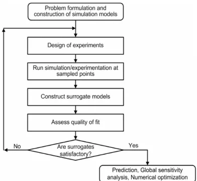
) represents both the approximation and measurement (random) errors.

Figure 1.1 summarizes the general statistical procedure to generate and use surrogates.

(25)

The internal steps of the loop can be detailed as:

1. Design of experiments: the design space is sampled in order to reveal its contents and tendencies (Owen, 1992; Morrsi and Mitchell 1995; and Montgomery, 1997). At this step, the gain of as much information as possible must be balanced with the cost of simulation/experimentation.

2. Run simulation/experimentation at sampled points: at this phase, the simulation (or experimentation) unfeasible regions of the design space can be revealed.

3. Construct surrogate models: the surrogate model is fitted to the collected data (Myers and Montgomery, 1995; Wasserman, 1993; Martin and Simpson, 2005; and Smola and Scholkopf, 2004). It may imply in the solution of a system of linear equations or even in the solution of an optimization problem.

4. Assess quality of fit: the precedent steps are sufficient to build a first tentative model, which overall quality and usefulness has to be evaluated by adequate sets of metrics (Box et al., 1978; Sacks et al., 1989; and Meckesheimer et al., 2002).

Table 1.1 shows several options for previously discussed techniques used in surrogate modeling.

Table 1.1. Techniques for surrogate modeling.

Technique Examples

Design of experiments

Factorial (full and fractional), Central Composite Design, Box-Behnken, D-optimal, Orthogonal Array, Latin Hypercube

Surrogate model Polynomial Response Surface, Radial Basis Neural Networks, Kriging Models, Support Vector Regression

Verification of model accuracy

Root mean square error, Maximum absolute error, Coefficient of correlation (using test points), Prediction sum of squares, Coefficient of determination ( ), Estimated prediction variance, Estimated process variance

2

R

1.2. Fundamental Concepts in Numerical Optimization

(26)

5

solution to a problem; instead, it means finding the more suitable solution to a problem (which is the case of compromise solutions and robust solutions). An example of an optimization problem is the following: maximize the profit of a manufacturing operation while ensuring that none of the resources exceed certain limits and also satisfying as much of the demand faced as possible. Thus, extending the previous discussion, the optimization work is a mathematical problem compound by the following elements (Haftka and Gürdal, 1992; Marler and Arora, 2004; and Vanderplaats, 2005):

• Design space: where all possible solutions for a problem are considered (also known as search space). Each element of the design space is called design variable. The vector of design variables, , is composed by the elements , which means that the number of design variables is

n

. The bounds of the design space are given by lower and upper limits for each design variable, . Design variables can be continuous (i.e., real values within a range), or discrete (i.e., certain values defined in a list of permissible values). When optimization is solved numerically, scaling design variables is important to avoid ill conditioning problems. This process consists in mapping the boundaries of each design variable to a new design space with boundaries [0 or .

x

i

, 1,

i

=

2,

…

,

n

dv

l u

v

− dv

, 1, 2, ,

i d

i i

x ≤x ≤ x i = … n

1] [ 1 1]

• Objective function: also known as cost function, fitness function or evaluating function. This is the way to evaluate each point of the design space. The objective function is denoted as

f

(

x

) for single objective problems and

f x

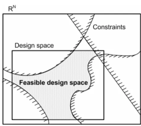
( ) for multi-objective problems.

• Constraints: impose restrictions to the system. A design point which satisfies all the constraints is called feasible, while a design point which violates even a single constraint is called infeasible. The collection of all feasible points is called feasible domain, or occasionally the constraint set. Figure 1.2 shows modifications in the original design space that are caused by constraints.

(27)

Figure 1.2. Design space definition.

In the single objective case, numerical optimization solves the following nonlinear, constrained problem: find the point, , in the design space that will minimize the objective function for a given set of system parameters, possibly observing a set of constraints. In other words, the standard formulation of an optimization problem is:

∗

x

(1.4)

( )

,

minimize

f

x

subject to:

(1.5) ( )

( )

1, 2, , , ,

0, 1, 2, , ,

1, 2, , ,

0, l u dv i i i j ineqcnstrt

ineqcnstrt ineqcnstrt cnstrt j

i n

x x x

g j n

j n n n

h ⎧⎪ ≤ ≤ = … ⎪⎪⎪⎪ _≤ ₌ _… ⎨⎪ ⎪⎪ = = + + … ⎪⎪⎩ x x u i where:

•

f

(

x

) is the objective function,

• xl_i ≤x_i ≤x imposes the side constraints to the design space, •

n

_dv is the number of design variables,

•

n

_ineqcnstrt is the number of inequality constraints,

•

n

_cnstrt is the total number of constraints (inequality and equality), and •

g

_j(

x

) and

h

_j(

x

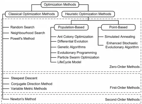
) are the inequality and equality constraints, respectively.

About the optimization algorithms, they can be classified according to the level of information required to solve the problem. This way, as it can be found in Vanderplaats (2005):

(28)

7

working with discrete design variables. The price paid for this generality is that these methods often require a large number of function evaluations.

• First-order methods: require the evaluation of the gradient of the functions. Since more information is used during the search, these methods are expected to be more efficient in terms of the number of function evaluations as compared with zero-order methods. However, the price paid is that gradient information must be supplied. In addition, they have difficulties to deal with local minima and discontinuity on the first derivatives.

• Second-order methods: use function values, gradient and the Hessian matrix (the square matrix of second order partial derivatives of a function). As they increase the amount of used information, they are expected to be more efficient. However, while it does not solve the difficulties with local minima, this fact also implies in the additional hardness of the Hessian computation.

Other than the level of information, the approach used by the algorithm to manipulate this information allows a second classification. In this sense, classical methods are based on Algebra and Differential Calculus. Alternatively, in heuristic methods, the most appropriate solutions of several found are selected at successive stages for use in the next step of the search. They are called heuristic methods since the selection and update of solutions follow a heuristic rather than a formal mathematical approach (Rasmussen, 2002; and Haupt and Haupt, 2004). Figure 1.3 shows a concise representation of both classifications for the optimization algorithms.

(29)

1.3. Classification of the Optimization Problems

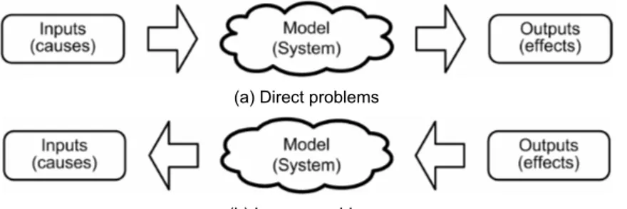
In terms of classification, in this research work, the optimization problems with continuous and eventually discrete-continuous variables are divided in two groups, namely direct problems and inverse problems. The distinction between them depends on the causes and effects relationship of the system. Figure 1.4 shows a scheme that illustrates the concepts in discussion. This way, in direct problems the inputs are used to determine either the best configuration of the given system or the response of the system to a pre-defined set of inputs. As an example of direct problems can be cited those in rigid body dynamics (in particular, articulated rigid body dynamics) that often require mathematical programming techniques, since rigid body dynamics attempts to solve an ordinary differential equation subjected to a set of constraints, which are various nonlinear geometric constraints such as “these two points must always coincide,” “this surface must not overlap to any other,” or “this point must always lie somewhere on this curve.” On the other hand, the inverse problem consists in using the results of actual observations to infer about either the values of the parameters characterizing the system under investigation or the inputs that generate a known set of outputs. As an example of inverse problems can be cited the identification of the proper boundary conditions and/or initial conditions such as: a) determination of thermal, stress/strain, electromagnetic, fluid flow boundary conditions on inaccessible boundaries, and b) determination of initial position, velocity, acceleration or chemical composition.

(a) Direct problems

(b) Inverse problems

Figure 1.4. Classification of problems according to the causes and effects context

In addition, some difficulties that are intrinsic to inverse problems may arise:

• an accurate model of the system is required, since the results of the identification procedure rely upon the model used;

(30)

9

• experimental data are incomplete either in the spatial sense (responses are available only in a limited number of positions along the structure), as in the time sense (responses are obtained in a given time interval and sampling frequency).

Alternatively, it is also possible that instead of finding the optimal set of values for different design variables, the optimization problem consists in finding the optimal combination of elements in a vector. As in the literature (Nemhauser and Wolsey, 1988; Papadimitriou and Steiglitz, 1998), here, these problems are classified as combinatorial optimization problems. In this category, instead of varying the values of each design variable, the optimizer changes the position of the design variables within the vector of design variables. The vehicle routing problem is an example of combinatorial optimization problem. Often the context is that of delivering goods located at a central depot to customers who have placed orders for such goods. The goal is minimizing the cost of distributing the goods, while serving the customers with a fleet of vehicles. Another example is the knapsack problem. It consists in the maximization problem of the best choice of essentials that can fit into one bag to be carried on a trip. Given a set of items, each with a cost and a value, the goal is to determine the number of each item to include in a collection so that the total cost is less than a given limit and the total value is as large as possible.

1.4. Literature Review

(31)

of an alkaline–surfactant–polymer flooding processes incorporating a local weighted average model of the individual surrogates. Goel et al. (2007) explored different approaches in which the weights associated with each surrogate model are determined based on the global cross-validation error measure called prediction sum of squares.

The literature about heuristic optimization algorithms is vast as well. Coello (2005) provided a brief introduction to this class of algorithm including some of their applications and current research directions. Van Veldhuizen and Lamont (2000) and Marler and Arora (2004) presented a survey of current continuous non-linear multi-objective optimization concepts and methods. Michalewicz (1995) and Coello (2002) reviewed methods for handling constraints by heuristic methods and tested them on selected benchmark problems; and discussed their strengths and weaknesses. About the algorithms themselves, especially those embraced in this research, Ant Colony Optimization is presented in details in Dorigo et al. (1996) and Pourtakdoust and Nobahari (2004); Differential Evolution is comprehensively discussed in Storn and Price (1997) and Kaelo and Ali (2006); Genetic Algorithms are well explained in Haupt and Haupt (2004) and Michalewicz and Fogel (2000); Particle Swarm Optimization is described in Kennedy and Eberhart (1995) and Venter and Sobieszczanski-Sobieski (2003); and finally, LifeCycle Optimization is introduced in Krink and Løvberg (2002) and recently applied to a real-word problem in Flores et al. (2007). Enhanced Stochastic Evolutionary Algorithm was first introduced by Saab and Rao (1991) and later applied to the optimization of the Latin hypercube design in Jin et al. (2005) and Viana et al. (2007c).

1.5. Scope of Current Research

In short, the goal of the present work is to develop methodologies for applying heuristic optimization techniques to the solution of optimization problems in Engineering. The research, conducted in the context of a doctoral thesis, has the following main objectives: • Study of the modern optimization techniques, embracing since the problem definition to

the solution of the optimization problem.

• Combining surrogate modeling and heuristic algorithms to the solution of optimization problems.

• Developing general-purpose optimization routines for academic use enabling its application to both direct and inverse problems.

(32)

11

(33)

(34)

CHAPTER II

SURROGATE MODELING AND NUMERICAL OPTIMIZATION

2.1. Introduction

Chapter I has already introduced the basic concepts on surrogate modeling and numerical optimization. This chapter discusses how the current doctoral research approached these techniques. This is done by presenting:

1. The interaction between the general user of numerical optimization and the set of components involved in the solution of an optimization problem.

2. The proper formulation of optimization algorithms and surrogate modeling techniques addressed by this research.

(35)

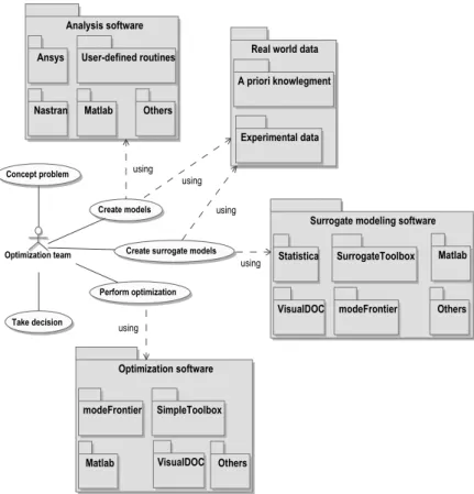
Surrogate modeling software SurrogateToolbox

modeFrontier VisualDOC

Statistica

Others Matlab

Optimization software

SimpleToolbox modeFrontier

VisualDOC Matlab Others Analysis software

User-defined routines Ansys

Nastran Matlab Others

Create surrogate models

Real world data A priori knowlegment

Experimental data

Perform optimization Concept problem

Optimization team

Create models

Take decision

using using using

using

Figure 2.1. Optimization environment.

More details are given below:

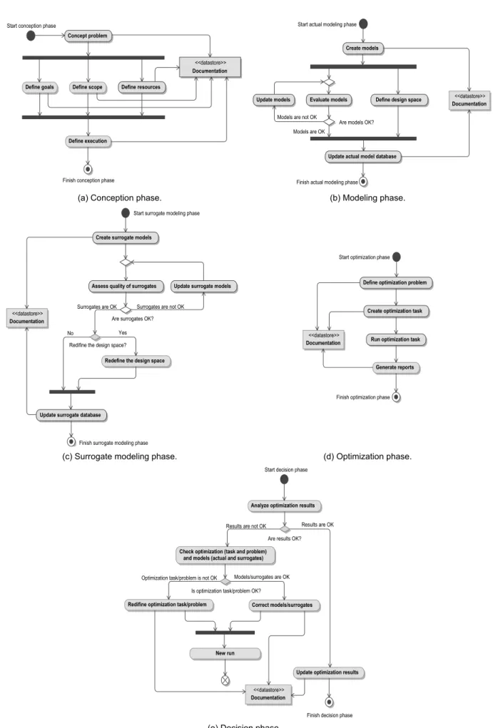
• Concept problem: this is the process through which goals, scope and resources are defined. The focus is on the needs and required functionality, documenting and then proceeding to design synthesis and system validation while considering the complete problem. This phase often involves contribution from diverse technical disciplines (not only Engineering but also resource management). Figure 2.2-(a) illustrates a possible flowchart for this phase.

(36)

15 <<datastore>> Documentation Concept problem Define resources Define execution Define scope Define goals

Start conception phase

Finish conception phase

Update actual model database Define design space Evaluate models

Update models <<datastore>>

Documentation Create models

Are models OK? Start actual modeling phase

Finish actual modeling phase Models are not OK

Models are OK

(a) Conception phase. (b) Modeling phase.

Assess quality of surrogates

Update surrogate database

Redefine the design space

Update surrogate models Create surrogate models

<<datastore>>

Documentation Are surrogates OK?

Redifine the design space?

Finish surrogate modeling phase

Start surrogate modeling phase

Surrogates are not OK

No Yes

Surrogates are OK

Define optimization problem

Create optimization task

Run optimization task

Generate reports

<<datastore>>

Documentation

Start optimization phase

Finish optimization phase

(c) Surrogate modeling phase. (d) Optimization phase.

Check optimization (task and problem) and models (actual and surrogates)

Redifine optimization task/problem

Analyze optimization results

Update optimization results Correct models/surrogates

New run

<<datastore>> Documentation Is optimization task/problem OK?

Are results OK?

Finish decision phase Start decision phase

Results are OK

Models/surrogates are OK Results are not OK

Optimization task/problem is not OK

(e) Decision phase.

(37)

• Create surrogate models: when the actual models are extremely expensive to be used, surrogate models are constructed. This phase is based on statistical procedures to replace the actual models. It frequently encompasses resources for building and evaluating the fidelity level of the resulting surrogate models. Figure 2.2-(c) exemplifies the sequence of activities in this phase.

• Perform optimization: in this phase the optimization problem is defined and solved. Figure 2.2-(d) suggests a possible scheme for this phase.

• Take decision: this procedure is supported by all previous ones. In a more general sense, practical considerations (such as investment, cost-benefit ratio, marketing trends) are combined with the results of the modeling and optimization phases. Here, the focus is given to the optimization process instead, as illustrated in Figure 2.2-(e).

Despite the beauty of each of the phases, this work addresses the aspects of the use of heuristic optimization techniques on the solution of engineering problems. It means that during the conception phase, the optimization team already decided to use this class of optimization algorithms.

2.2. Surrogate Modeling Framework

2.2.1. Design of Experiments (DOE) and Latin Hypercube Sampling

(38)

17

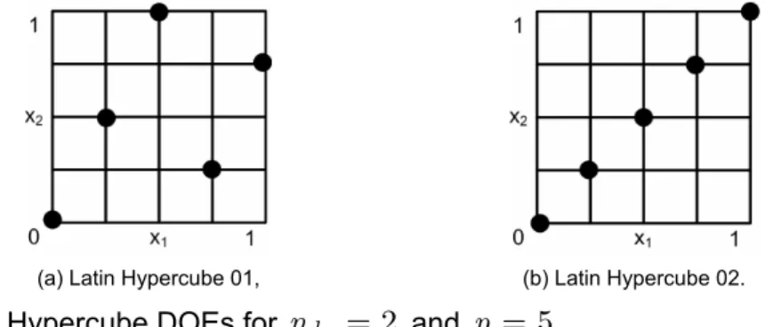
The Latin Hypercube design is constructed in such a way that each one of the dimensions is divided into equal levels and that there is only one point for each level (Bates et al., 2004). The final Latin Hypercube design then has samples. Figure 2.3 shows two possible Latin Hypercube designs for and . Note that the Latin Hypercube design is constructed using a random procedure. This process results in many possible designs, each being equally good in terms of the Latin Hypercube conditions. However, a design that is ill suited for creating a surrogate model is possible, even if all the Latin Hypercube requirements are satisfied, as illustrated in Figure 2.3.

dv

n

p

2

dv

n

=

p

=

5

(a) Latin Hypercube 01, (b) Latin Hypercube 02.

Figure 2.3. Latin Hypercube DOEs for

n

dv

=

2

and

p

=

5

.

To overcome the above mentioned problem, the Optimal Latin Hypercube design was introduced to improve the space-filling property of the Latin Hypercube design. The Optimal Latin Hypercube design augments the Latin Hypercube design by requiring that the sample points be distributed as uniformly as possible throughout the design space. Unfortunately, the Optimal Latin Hypercube design results in a hard and time consuming optimization problem. For example, to optimize the location of 10 samples in dimensions, the optimizer has to select the best design from more than 1022 possible designs. If the number of design variables is increased to

5

, the number of possible designs is more than . To solve the Optimal Latin Hypercube design, it is necessary to formulate an optimization problem, the solution of which is the best design. To have an idea about how difficult this task can be, Ye et al. (2000) reported that generating an Optimal Latin Hypercube design with 25 samples in dimensions using a column-wise/pair-wise algorithm could take several hours on a Sun SPARC 20 workstation. The Optimal Latin Hypercube was a case study of combinatorial optimization during this doctoral research. The achieved advances were reported in Viana et al. (2007a), where the generation of an Optimal Latin Hypercube design with samples in dimensions was as fast as

5

minutes in a PC with a 1000 MHz Pentium III Zeon processor. Chapter V gives more details about this implementation.

4

32

6 10

×

4

(39)

2.2.2. Surrogate Modeling Techniques

Viana et al. (2008a) have already shown that, for prediction purposes, it pays to generate a large set of surrogates and then pick the best of the set according to an estimator of the root mean square error called PRESS (prediction sum of squares). The main features of the four surrogate models used in this study are described in the following sections. For all discussion, consider that the models are fitted with the set of samples.

p

1. Kriging (KRG)

Kriging is named after the pioneering work of the South African mining engineer D.G. Krige. It estimates the value of a function as a combination of known functions (e. g., a linear model such as a polynomial trend) and departures (representing low and high frequency variation components, respectively) of the form:

( ) i

f

x

(2.1)

( ) ( ) ( )

1

ˆ

,

p i i i

y

β

f

Z

=

∑

+

x

)

where is assumed to be a realization of a stochastic process with zero mean, process variance , and spatial covariance function given by:

( )

Z

x

2

σ

(2.2)

( )

₍

₎

(

)

2

(

cov Z xi ,Z xj = σ R x xi, j , where R

(

x xi, j

)

is the correlation between

x

i and

x

j.

The conventional KRG models interpolate training data. This is an important characteristic when dealing with noisy data. In addition, KRG is a flexible technique since different instances can be created, for example, by choosing different pairs of and correlation functions. The complexity of the method and the lack of commercial software may hinder this technique from being popular in the near term (Simpson et al., 1997).

( ) i

f

x

The Matlab code developed by Lophaven et. al (2002) was used to execute the KRG algorithm. More details about KRG are provided in Sacks et al. (1989), Simpson et al. (1997), and Martin and Simpson (2005).

2. Polynomial Response Surface (PRS)

(40)

19

(2.3)

( ) ₀

1 1 1

ˆ

,

m m m

i i ij i j

i i j

y

β

x

β

= = =

=

+

∑

+

∑ ∑

x

x x

The set of coefficients can be obtained by least squares and according to the PRS theory are unbiased and have minimum variance. Another characteristic is that it is possible to identify the significance of different design factors directly from the coefficients in the normalized regression model (in practice, using t-statistics). In spite of the advantages, there is a drawback when applying PRS to model highly nonlinear functions. Even though higher-order polynomials can be used, it may be too difficult to take sufficient sample data to estimate all of the coefficients in the polynomial equation, particularly in large dimensions.

β

The SURROGATES toolbox of Viana and Goel (2008) was used for PRS modeling. See Box et al. (1978) and Myers and Montgomery (1995) for more details about PRS.

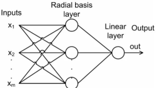
3. Radial Basis Neural Networks (RBNN)

RBNN is an artificial neural network which uses radial basis functions as transfer functions. RBNN consist of two layers: a hidden radial basis layer and an output linear layer, as shown in Figure 2.4.

Figure 2.4. Radial basis neural network architecture.

The output of the network is thus:

(2.4)

( ) ( )

1

ˆ

,

N

i i

i

y

a

ρ

=

∑

x

c

,

where

N

is the number of neurons in the hidden layer, is the center vector for neuron

i

, and are the weights of the linear output neuron. The norm is typically taken to be the Euclidean distance and the basis function is taken to be the following:

i

c

i

a

( , i) exp

(

2

)

(41)

where

exp

( )

⋅

is the exponential function.

RBNN may require more neurons than standard feed-forward/back-propagation networks, but often they can be designed in a fraction of the time it takes to train standard feed-forward networks. They work best when many training points are available, and this can be a crucial drawback in some applications. Another important point to consider is that the training process may lead to totally different configurations and thus different models.

The native neural networks Matlab® toolbox (MathWorks Contributors, 2002) was used to execute the RBNN algorithm. RBNN is comprehensively presented in Smith (1993), Wasserman (1993), and Cheng and Titterington (1994).

4. Support Vector Regression (SVR)

SVR is a particular implementation of support vector machines (SVM). In its present form, SVM was developed at AT&T Bell Laboratories by Vapnik and co-workers in the early 1990s (Vapnik, 1995). In SVR, the aim is to find that has at most

ε

deviations from each of the targets of the training inputs. Mathematically, the SVR model is given by:

( )

ˆ

y

x

(2.6) ( )

(

)

( ) 1 ˆ , p

i i i

i

y a a∗ K

=

∑

− +

x x x b

)

where is the so-called kernel function, are different points of the original DOE and is the point of the design space in which the surrogate is evaluated. Parameters

, , and

b

are obtained during the fitting process.

( i

,

K

x x

x

_i

x

i

a

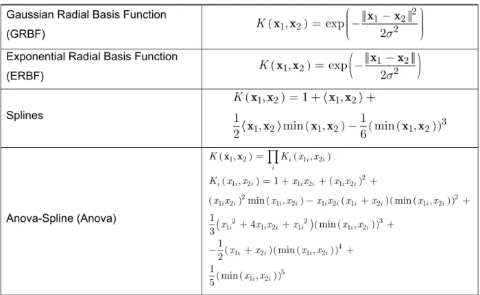
i∗

Table 2.1 lists the kernel functions used in this work.

During the fitting process, SVR minimizes an upper bound of the expected risk unlike empirical risk minimization techniques, which minimize the error in the training data (which defines , , and

b

in Eq. (2.6)). This is done by using alternative loss functions. Figure 2.5 shows two of the most common possible loss functions. Figure 2.5-(a) corresponds to the conventional least squares error criterion. Figure 2.5-(b) illustrates the loss function used in this work, which is given by:

i

a

i∗

( )

( ) ( )

ˆ

, if

ˆ

, otherwise

y

Loss

y

ε

−

≤

ε

⎧⎪⎪

=

_⎨⎪

−

⎪⎩

x

(42)

21

Table 2.1. Kernel functions (consider

exp

( )

⋅

as the exponential function).

Gaussian Radial Basis Function

(GRBF) ( )

2

1 2

1

,

2

exp

₂

2 K

σ

⎛

₋

⎞

_⎟

⎜

=

⎜

_⎜

−

⎟

_⎟

⎝

⎠

x

x x

Exponential Radial Basis Function

(ERBF) ( )

(

)

1 2

1, 2 exp ₂

2

K

σ −

= − x x

x x

Splines

( )

( ) ( ( ))

1 2 1 2

3

1 2 1 2 1 2

,

1 ,

1

1 ,

min

,

min

,

2

6 K

= +

+

−

x x

Anova-Spline (Anova) ( ) ( ) ( ) ( ) ( ) ( ) ( )( ( ))

(

)

( ( )) ( )( ( )) ( ) ( )

1 2 1 2

2

1 2 1 2 1 2

2 2

1 2 1 2 1 2 1 2 1 2

3

2 2

1 1 2 1 1 2

4

1 2 1 2

5 1 2

, ,

, 1

min , min ,

1

4 min ,

3 1 min , 2 1 min , 5

i i i i

i i i i i i i

i i i i i i i i i i

i i i i i i

i i i i

i i

K K x x

K x x x x x x

x x x x x x x x x x

x x x x x x

x x x x

x x = = + + + − + + + + + − + +

∏

x x

The implication is that in SVR the goal is to find a function that has at most deviation from the training data. In other words, the errors are considered zero as long as they are inferior to

ε

.

ε

According to Smola and Scholkopf (2004): “after that the algorithmic development seems to have found a more stable stage, one of the most important ones seems to be to find tight error bounds derived from the specific properties of kernel functions.” Another open issue in SVR is the choice of the values of parameters for both kernel and loss functions.

(a) Quadratic (b) ε- insensitive

Figure 2.5. Loss functions.

(43)

5. Using a Large Set of Surrogates

Before start the discussion about the use of an ensemble of surrogates, it is important to clarify that when a set of surrogates is generated a common measure of quality must be employed in order to rank the surrogates. Since the set may be constituted by surrogates based on different statistical assumptions, this measure must be model-independent. One commonly used measure is the root mean square error (

RM

), which in the design domain with volume

V

is given by:

SE

( ) ( )

[ ]2

1

ˆ ,

V

RMSE y y d

V

=

∫

x − x x (2.8)

RMSE

is computed by Monte-Carlo integration at a large number of

p

_test test points:

( )2

1

1 ˆ

test

p

i i

test i

RMSE

y

p

₌

=

∑

−

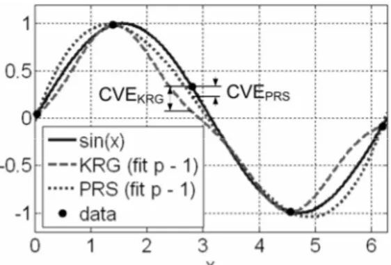
(2.9)

However, the use of an extra large set of test points is frequently prohibitive in most of the real world applications. This way, is estimated by using cross-validation errors. A cross-validation error is the error at a data point when the surrogate is fitted to a subset of the data points not including that point. When the surrogate is fitted to all the other

points, (so-called leave-one-out strategy), it is obtained the vector of cross-validation errors, . This vector is also known as the

PR

vector ( stands for prediction sum of squares). Figure 2.6 illustrates the cross-validation errors at the third point of the DOE by fitting a PRS and a KRG model to the remaining four of the five data points of the function sin(x).

RMSE

1 p

−

e

ESS

PRESS

(44)

23

However, the leave-one-out strategy is computationally expensive for large number of points. We then use a variation of the k-fold strategy (Kohavi, 1995). According to the classical k -fold strategy, after dividing the available data (p points) into p/k clusters, each fold is constructed using a point randomly selected (without replacement) from each of the clusters. Of the k folds, a single fold is retained as the validation data for testing the model, and the remaining k – 1 folds are used as training data. The cross-validation process is then repeated k times with each of the k folds used exactly once as validation data. Note that k -fold turns out to be the leave-one-out when k = p.

The

RM

SE

is estimated from the

PR

ESS

vector:

2

1

1 ,

p

RMS i

i

PRESS

e

PRESS

p

=

∑

=

,

(2.10)

where

e

_i is the cross-validation error obtained at the i-th point of the DOE.

As shown in Viana et al. (2008b), since is a good estimator of the , one possible way of using multiple surrogates is to select the model with best value (called in the literature as

Be

surrogate). Because the quality of fit depends on the data points the

Be

surrogate may vary from DOE to DOE. This strategy may include surrogates based on the same methodology, such as different instances of Kriging (e.g., Kriging models with different regression and/or correlation functions). The main benefit from a diverse and large set is the increasing chance of avoiding (i) poorly fitted surrogates and (ii) DOE dependence of the performance of individual surrogates. Obviously, the key for the success when using is the quality of the

estimator.

RMS

PRESS

RMSE

PRESS

stPRESS

BestPRESS

PRESS

The SURROGATES toolbox of Viana and Goel (2008) is used for an easy manipulation of all different codes previously presented.

2.3. General Optimization Problem

(45)

(2.11)

( )

,

minimize

f x

subject to:

(2.12) ( )

( )

1, 2, , , ,

0, 1, 2, , ,

1, 2, , ,

0, l u dv i i i j ineqcnstrt

ineqcnstrt ineqcnstrt cnstrt j

i n

x x x

g j n

j n n n

h ⎧⎪ ≤ ≤ = … ⎪⎪⎪⎪ _≤ ₌ _… ⎨⎪ ⎪⎪ = = + + … ⎪⎪⎩ x x ⎤⎥⎦ u i where:

• is the vector of objective functions. This

vector is composed by objective functions that can sometimes support but more commonly conflict with each other.

( ) ₁( ) ₂( ) ( )

obj

T n

f f f

⎡

= _⎢⎣

f x x x … x

• xl_i ≤x_i ≤x imposes the side constraints to the design space, •

n

_dv is the number of design variables,

•

n

_ineqcnstrt is the number of inequality constraints,

•

n

_cnstrt is the total number of constraints (inequality and equality), and •

g

_j(

x

) and

h

_j(

x

) are the inequality and equality constraints, respectively.

Figure 2.7 gives a graphical representation of the general optimization problem in terms of design and function space.

Figure 2.7. General optimization problem.

(46)

25

This is known as “Pareto optimally” (Haftka and Gürdal, 1992; Marler and Arora, 2004). Formally, the Pareto optimal can be defined as follows (Marler and Arora, 2004):

• A point, , is a Pareto optimal if there does not exist another

point, , such that for all ,

and for at least one objective function.

FeasibleDesignSpace

∗

_∈

x

FeasibleDesignSpace

∈

x

f

_i(

x

)

≤

f

_i

(

x

∗

)

∗

x

1, 2,

,

obj

i

=

…

n

( )

(

i i

f

x

<

f

The set of Pareto optimal points creates what is typically referred to as the Pareto front. Another important concept in multi-objective optimization is the concept of utopia point (Marler and Arora, 2004):

• A point, , is an utopia point (or ideal point) if for each

, .

( )

∈

FeasibleObjectiveSpace

f

x

1, 2,

,

obj

i

=

…

n

f

_i (

x

)

=

min

(

f

_i(

x

))

In general, the utopia point is unattainable, and the best solution is as close as possible to the utopia point. Such a solution is called a compromise solution and is Pareto optimal. Figure 2.8 illustrates these concepts by considering the example of two conflicting objectives. The shaded area defines non-optimal solutions.

Figure 2.8. Pareto front.

As in the case of design variables, performing a mapping of the functions to a common range may be convenient. By doing this, they will not be erroneously interpreted when combined together by the handling techniques. There are different methods of scalarization, depending on whether a function is an objective or a constraint.

Considering the objective functions, the first approach is as simple as:

( )

maxi ,

i

f f

f

= x

x

(47)

where is the scaled version of and is the maximum value possible for . Note that is assumed. The result, , is a non-dimensional objective function with an upper limit of one (or negative one) and an unbounded lower limit.

( ) i

f

x

f

_i(

x

) max( )

i

f

x

( ) i

f

x

max( )

0

i

f

x

≠

f

_i(

x

)

An alternative to Eq. (2.13) is:

( ) ( ) ( ) ( ) . i i i i f f f f −

= x x

x

x (2.14)

In this case, the lower value of is restricted to zero, while the upper value is unbounded.

( ) i

f

x

However, a most robust approach is given as follows:

( )

( ) ( )

maxi i .

i i i f f f f f − = − x x x

x x (2.15)

In this case, the values assumed by

f

_i(

x

) are between zero and one.

It is easy to see that the mapping as suggested by Eqs. (2.13) to (2.15), relies on and . Unfortunately, this information is not available. Indeed, there might be no reason for optimization if was known. In practice, these values are either estimated or assumed as based on any a priori knowledgement regarding the problem. Vanderplaats (2005) suggests as the objective function associated with the initial design (also called baseline design) to replace ; and as the desired value of this objective function to be used in the place of . The counterparts on the case of heuristic optimization algorithms are the worst value of the objective function found in the initial population as suggestion for , and in the case of lacking an initial guess for , the best value found in the initial population for could be used as .

( )

max

i

f

x

f

_i (

x

)

( ) i

f

x

( ) worst i f x ( ) max i

f

x

f

_i∗(

x

)

( ) i

f

x

( ) i

f

x

( ) worst i f x ( ) i

f

∗

x

f

_i(

x

)

f

_i∗(

x

)

As in the case of objective functions, inequality constraint functions can also lie in different ranges. Then, when treated by penalty methods (as explained later), that can be misinterpreted as different level of violation instead of different ranges. In that case, it is desired that the scaled versions of the constraints have the same range (or order of magnitude) while restoring the formulation as presented in Eq. (2.12). Thus, assuming that an inequality constraint is as g_j(x)≤g∗_j, there are just two possibilities for the target value,

j

(48)

27 ( ) ( ) 0 , j j j g g g•

= x ≤

x (2.16)

where

g

_j(

x

) is the scaled version of

g

_j(

x

), and g_j• is its order of magnitude. For the second case, i.e. gj∗ ≠ 0,

g

_j(

x

) is computed using:

( )

1 0 .

j j j g g g∗

= x − ≤

x (2.17)

On other circumstances, the optimum must satisfy g_j(x)≥g_j∗, and as before, the scaled version depends on g_j∗. For gj∗ = 0, the scaled version is given by changing the inequality on Eq. (2.16). For gj∗ ≠ 0, the scaled version is as:

( )

1 j 0 .

j

g g

g∗

= − x ≤

x (2.18)

Finally, for the same reasons, re-writing the set of equality constraints may be convenient. If the target value of

h

_j(

x

) is h_j∗ = 0, the scaled version, h_j(x), is as:

( ) ( ) 0 , j j j h h h•

= x =

x (2.19)

where h_j• is the order of magnitude of

h

_j(

x

).

If on the other hand, hj∗ ≠ 0, then h_j(x) is given by:

( ) ( ) 1 0 j j . j h h h∗

= x − =

x (2.20)

Now that all functions considered in the optimization problem have been properly scaled, the general optimization problem can be re-stated to be solved by using heuristic optimization algorithms. Equations (2.11) and (2.12) are combined in a functional, , to be minimized. This functional is obtained as follows (Marler and Arora, 2004):

( )

J

x

(2.21) ( )

(

( )

)

(

( ), ( )

(49)

where plays the role of the multi-objective handling technique that combines the vector of scaled objective functions, , and plays the role of the constrained optimization handling technique that combines the vectors of scaled inequality constraints, , and equality constraints, . is zero, if no violation occurs, and positive otherwise (actually, the worst the violation the larger the value of

). ( )

(

F f x

)

⎤⎥⎦

( )

f x

P

(

g x( ),h x( )

( )

g x

h x

( ) P

(

g x( ),h x( )

( ) ( )

(

,

)

P g x h x

2.4. Multi-Objective Optimization Techniques

When considering multi-objective problems, the algorithms offer alternatives either to compute the compromise solution (Van Veldhuizen and Lamont 2000; and Marler and Arora, 2004) or to build the Pareto front (Zitzler and Thiele, 1999; and Deb, 2001). In this work, the focus is on algorithms used to obtain the compromise solution.

Basically, there are two main strategies used for these techniques. The first consists in building a functional through the manipulation of the objective functions. The second one redefines the multi-objective problem as a constrained optimization problem. For the sake of simplicity, in this work only the most common methods following the first approach are covered.

2.4.1. Weighted Sum Method

This is the most common approach used in multi-objective optimization. The functional is given by:

( )

(

F f x

(2.22) ( )

(

)

( ) 1 , obj n i i i

F w f

=

∑

f x x

where is the vector of weighting factors, which indicate the

importance of each objective, such as and .

1 2 obj

T n

w w w

⎡ = _⎢⎣ w … 1 1 obj n i i w = =

∑

w

i

SURROGATE MODELING TECHNIQUES AND HEURISTIC OPTIMIZATION METHODS APPLIED TO DESIGN AND IDENTIFICATION PROBLEMS

FELIPE ANTONIO CHEGURY VIANA

SURROGATE MODELING TECHNIQUES AND

HEURISTIC OPTIMIZATION METHODS APPLIED TO

DESIGN AND IDENTIFICATION PROBLEMS

UNIVERSIDADE FEDERAL DE UBERLÂNDIA

FACULDADE DE ENGENHARIA MECÂNICA

SURROGATE MODELING TECHNIQUES AND HEURISTIC

OPTIMIZATION METHODS APPLIED TO DESIGN AND

IDENTIFICATION PROBLEMS

Tese

apresentada ao Programa de

Pós-graduação em Engenharia Mecânica da

Universidade Federal de Uberlândia, como parte

dos requisitos para a obtenção do título de

DOUTOR EM ENGENHARIA MECÂNICA.

Área de Concentração:

Mecânica dos Sólidos

e Vibrações

Orientador: Prof. Dr. Valder Steffen Jr.

ACKNOWLEDGMENTS

SURROGATE MODELING TECHNIQUES AND HEURISTIC OPTIMIZATION

METHODS APPLIED TO DESIGN AND IDENTIFICATION PROBLEMS

TABLE OF CONTENTS

Thesis

Abstract

Resumo

Nomenclature

f

x

f x

g

x

h

x

n

n

n

x

x

x

ith

y

x

ˆ

y

x

f

x

f

x

g

x

g

x

h

x

h

x

n

p

BestPRESS

PR

ESS

J

x

RMSE

c

c

n

CR

DM

F

P

γ

σ

ˆ

δ

x

y

_ith