Evolutionary Design of Engineering Constructions
Abstract
The basic information required to utilize one of possible computation tools/algorithms (mainly the evolution strategy) to solve a wide class of real practical engineering optimization problems is presented and discussed in the present paper. The effectiveness of the considered method is demonstrated by the possibility of the use of different form of objective functions, various and numerous nonlinear constraints and different types of design variables (continuous, discrete, real, integer). The sensitivity of the algorithm to the choice of the evolution strategy parameters is also discussed herein. The generality of the evolution strategy is illustrated by the analysis of various examples dealing with: the design of helical springs, the buckling of cylindrical composite panels and the buckling of pressure vessels with domed heads.
Keywords
optimal design; evolutionary algorithms, buckling; plated and cylindrical composite panels; pressure vessels, helical springs, strength of laminates.
I. Introduction
It is well-known that the necessity of optimal design can arise in a natural way in various scientific/research fields. The search for better solutions is perhaps as old as mankind itself. Therefore the formulation of an optimization problem is well-known and well-defined in mathematical terms. However, there is still an open problem dealing with the selection of the most flexible and convenient tool for searching for the optimum which is usually called as an optimization algorithm. The algorithms for solving the real engineering problems are very complicated and in order to obtain practical solutions a significant computational effort is needed. Therefore, complex practical problems cannot be found with the use of classical methods. Over the last thirty years, different heuristic methods were formulated. H.Wilf [1] explains the sense of those algorithms in the following way: “…methods that seem to work well in practice, for reasons nobody understands…”.
Optimization algorithms (methods) can be classified in different groups. One of possible classifications is given below. It combines both classical and modern approaches, including different types of heuristics.
Combinatorial methods [2] – all possible solutions (combinations – each variable takes one of a finite set value) of the problem are analyzed.
Deterministic optimization problems [3] (such as e.g. hill climbing and others) are commonly well-defined in terms of rigorous mathematical analysis. They are based on a series of axioms dealing with the linearity, convexity, unimodality (one optimum), differentiability and connectivity of the problem. Usually, the objective is given in an analytical form, and the solution is a unique one. In addition, the design space is a small one.
Stochastic analysis (e.g. mathematical programming [2,3], ant colony optimization [4-8], immune system methods [9], memetic algorithms [10], scatter search & path relinking [11,12], particle swarm [13-16], genetic algorithms [17-21], differential algorithms [2,3]) is based on the random search for the optimum. In general, the optimum solution can be be determined as the best solution only, and usually not as a global optimum. Therefore, optimal solutions are sometimes called as quasi-optimal.
Mixed algorithms (se for instance Refs [22-30] and especially chaotic neural networks [31-36]) combine the best features of the deterministic and stochastic analysis. The optimal solutions are independent on an initial information. They are effective in the sense of possibility of finding global unimodal or multi-modal optimal solutions for extremely hard, often poorly specified problems. The analytical description of the problem is not required in order to find a global optimum – they may work as a black box. On the other hand, the computational effort is reduced to the minimum.
Aleksander Muc*
Institute of Machine Design, Cracow University of Technology, Kraków, Poland. E-mail: [email protected]
*Corresponding author
http://dx.doi.org/10.1590/1679-78254947
In the late 60s several researchers focused their attention and invented a new type of optimization methods that are called now as evolutionary algorithms (EAs). Now, those techniques are also known under the name
metaheuristics [37].
Therefore, the proposed herein method of the classification is not a unique, and, of course, is one of possible proposals. However, it demonstrates evidently the present tendency of the optimization strategy in the sense of the search for the convenient mixed algorithms having the highest effectiveness and robustness in the multimodal optimization problems with objective functions evaluated in a numerical way. Such a group of algorithms is also suitable for solving discrete optimization problems arising with the use of design codes constituting a discrete space of design variables. It is well-known that no optimization method is better to any other. A broader discussion of those problems is presented e.g. in Ref [38]. However, not trying to propose better methods is an erroneous conclusion.
Taking the above remarks into consideration we intend to build an optimization algorithm that can solve a broad class of engineering problems encountered in practice, possessing a large number of design parameters (integer, discrete, continuous and integer/discrete-continuous) and a large number of constraints. Genetic algorithms (GA) has been highly successful as one of evolutionary computation techniques in searching for a broad class of stacking sequence, size, topology optimization problems for composite structures (see Refs [39-41]). However, the application of that optimization technique is limited to a very few inequality constraints only. Now, our attention will be particularly focused on the formulation of the alternative to GA evolutionary computation optimization technique. It is based on the idea of the evolution strategy so that the proposed algorithm allows us to eliminate the problems associated with taking into account a large number of constraints.
In details, the main objective of the present considerations will be two-fold:
1. To present the classification of evolutionary algorithms and the actual terminology dealing with the application of evolutionary algorithms in the structural optimization problems in order to emphasize their differences and similarities and on the other hand to eliminate ambiguities and misunderstandings arising with the use of the improper term “evolutionary optimization” – see e.g. Ref [42]. In fact, the term evolutionary refers to one individual part of the optimization process and directly to an optimization algorithm only what is clearly underlined in Ref [43]
2. To illustrate the generality, effectiveness and accuracy of the described herein, completely new evolution strategy that is based on the appropriate analysis of constraints (feasible regions).
II. Evolutionary Computation
Now, in all branches of sciences an evolutionary computation plays a very special and significant role among various optimization algorithms. By many researchers the evolutionary computation area is divided in four specific domains: (i) genetic algorithms (GAs), (ii) evolutionary programming (EP), (iii) evolution strategies (ESs), (iv) genetic programming (GP).
In fact, now, hybrid of the above-mentioned four algorithms (metaheuristics) are employed in the analysis. Implementing evolutionary algorithms a series of operations should be taken into considerations. They are summarized in Table 1. However, it is necessary to point out that all operations that are conducted in four groups of evolutionary computations have their own meaning and are different. For instance, it is impossible to give the identical meaning of the reproduction or the crossover or the recombination operations. In genetic algorithms reproduction means the selection of individuals from the initial populations using only the fitness value. Thus, for instance having the size of the initial population equal to 10 and having randomly generated 10 different individuals, after reproduction 5 different individuals only may create a population having the same size as previously, i.e. equal to 10. Then, the crossover operation may be conducted. As it may be seen those operations are not connected with the form of chromosomes. In addition, it is worth to emphasize that according to the standard [43] recombination has a different meaning than crossover since crossover is limited to so-called sexual recombination only. In general, the use of different terms in the brief presentation of evolutionary algorithms should demonstrate different operations and the difference in specific groups of evolutionary computations.
The foundation of genetic algorithms (in 1950s) is connected with the name of the biologist A.S. Fraser [44]. J. H. Holland [45] (1962) with the students (K.A. De Jong, D. E. Goldberg) have had the greatest influence on the developments of GAs.
In 1966 L. J. Fogel et al. [46] presented a new idea called now as evolutionary programming. The lack of a crossover operation is a characteristic feature of this method.
The last major method of EC was founded by R. M. Friedberg [49] (called as genetic programming) and it is joined directly and particularly with the work on the length of computer programs.
Table 1. Operations Carried out in EAs
GA EP ES GP
begin the analysis fitness of individuals reproduction of
individuals conduct crossover carry out mutation return to step 2 or finish operations
begin the analysis fitness of individuals carry out random
mutation define new
children selection of new
members return to step 2 or
finish operations
begin the analysis conduct operations of recombination carry out mutation
define new children selection of new
members finish operations or return to step 2
begin the analysis fitness of programs reproduction of
individuals conduct crossover
operations finish operations or return to step 2
As it may be noticed GA, EP, ES and GP can be characterized by a variety of qualities in common, although they also differ in a sequence of operations and the termination of operations. Differences between all four of them seem to become more and more indistinct.
III. Optimization Problem Formulation
An arbitrary engineering problem dealing with the optimal design has three fundamental common features, such as: 1) selection one or more design variables, 2) choosing an objective function, 3) identification a set of equality or inequality constraints. In our problem design variables can be described as the vector x having I components xi (i=1,2,…,I). It is also assumed that each component, dependent on the problem considered, can
belong to a set of natural, discrete or real numbers. A discrete set of numbers corresponds directly to constraints existing in various codes where dimensions of real products are not continuous but discrete real numbers. All components of the vector x must be positive as variables corresponding to real dimensions of constructions. They are constrained by lower and upper limits – Eq. (1), i.e.:
0
L Ui i i
x
x x
(1)To simplify numerical computations they are normalized in the following manner – Eq. (2):
/
N L U L
i i i i i
x
x x
x
x
(2)The constraints are given in the inequality or equality form – Eq. (3):
( ) 0,
1,2,...,
j
g x
j
J
,h x
k( ) 0,
k
1,2,...
K
(3)Now, one objective function is analyzed only and it is always formulated as searching for the maximum of the objective function F – Eq. (4), i.e.:
( )
Max F x
(4)In a classical manner all Min or MinMax optimization problems can be transformed to the above.
IV. Description of the Evolution Strategy
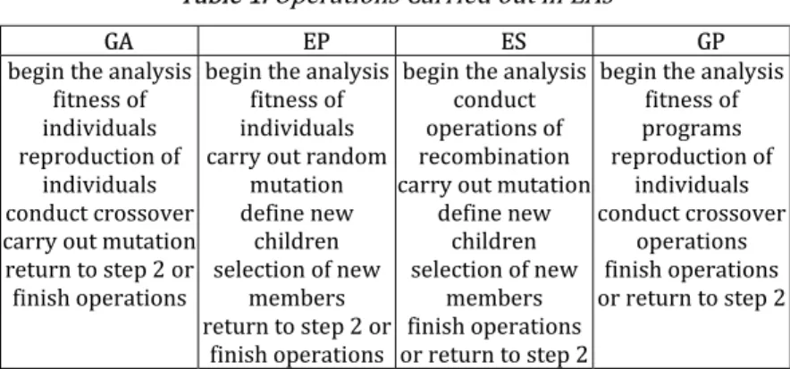
According to Rechenberg’s [50] conclusions the field of evolution strategies can be characterized as the evolution of evolution. Usually, the evolution strategies utilize three types of operations: 1) recombination – Eqs (5), (6), 2) mutation – Eq. (7) and 3) selection.
During the recombination operation (see Fig.1) the child xinew can be obtained by:
B
i A i new i xx
x (5)
- the intermediate recombination )
migr , vel ; x x ( R x
x A
i B i A i new
i (6)
R denotes a function and vel, migr are called as strategy parameters.
2 children migr=2, vel2 4 children migr=4, vel1
xB
xA
vel1 vel2
x1new
x2new
Figure 1. Description of the recombination operations
All new children (particles in Fig.1) should satisfy all equality or inequality constraints (3). In the present formulation the restoration method is used – see Fig.2. Other methods are described e.g. in Ref [51]. In general, the restoration method is based on returning back new produced children to the boundary by a simple operation that can be written in the following way:
new0
new1new
new0
j j
if g x
x
is replaced byx
such that g x
(7)4 children migr=4, vel
xB
xA vel x
new Boundary gj(x1new)=0
Figure 2. The restoration method
The optimization process is terminated as for the assumed objective function F the following condition is satisfied:FbestFworst for all members of the population.
The broader description of all assumptions and procedures introduced in the proposed version of the evolution strategy can be found e.g. in Ref[53].
V. Applications of the Proposed Algorithm - Numerical Examples
In this section we intend to show how the proposed algorithm works in some engineering problems. They are limited to the analysis of isotropic and 2D composite structures and mainly devoted to the cost optimization problems understood in the sense of the volume optimization (minimization) problems. In general, we intend to demonstrate how the algorithm works as the various types of inequality constraints exists. They number is even higher than the number of design variables but such a problems are typically encountered in engineering practice. It should be mentioned also that the field of possible applications is (and can be) much higher.
A. Design of Helical Springs
In various engineering applications helical compression springs constitute an important element. It is well-known that they not only can exert external compressive force but also provides the structural flexibility and can store or absorb energy. In the machine design such elements should satisfy a lot of various mechanical requirements. For helical springs the optimization problem can be formulated in the following manner: to minimize the total volume (weight) of the spring. The volume of the spring is the sum of the volume of active and inactive coils.
2 2
/ 4
Min
N Q Dd
(8)where the symbols N, Q denotes the number of active coils, and the number of inactive coils, respectively. Q is a constant and it is assumed to be equal to 2. D is the mean coil diameter, whereas d is the wire diameter (see Fig. 3). In order to use the consistent notation three variables (N, D, d) in Eq. (8) will be treated as the design variables and are denoted by xi (i=1,2,3), respectively.
There are seven constraints for this problem – Eqs (9)-(16): maximum allowable stresses:
3max max
8
F DK
w/
d
,K
w
4
C
allow
1 / 4
C
allow
4 0.615 /
C
allow, (9) allowable length:max
max
105(
)
100
F
N Q d l
k
, 348
Gd
k
D N
, (10)lower limit on wire diameter: min
d
d
, (11)maximum allowable outside diameter: max
D D
, (12)allowable spring index:
3
C
allow
D d
, (13)pocket length:
max
/
0
w p
l
F
F
k
, (14)clash allowance:
/
0,
p pm
where Kw is the Wahl correction factor, Fmax=4.45 [kN], τmax=1303 [MPa], lmax=356 [mm], dmin=5.08 [mm],
Dmax=76.2 [mm], Fp=1.334 [kN], lpm=152.4 [m], maximum spring length at maximum force lw=31.75 [mm],
Kirchhoff's shear modulus G=79.3 [GPa].
Figure 3. Helical compression spring
The bounds for the analyzed problem have been chosen in the following way:
1,
max min
,
3
min,
max
,
min,
max/ 3
N
l
d
D
d
D
d
d
D
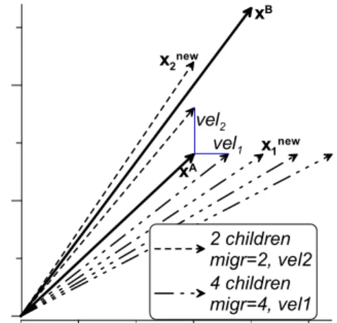
(16)Table 2. Comparison of optimal results – real design variables. Sandgren
[54] Present results
N 9.1918 7.117651855843154
D [mm] 30.61208 34.85906690200768 d [mm] 7.14756 7.390511146897453 Objective function (8) in
[mm3] 43184.8297592 42833.88535256481
0 0.25 0.5 0.75 1 x1 0 0.25 0.50.75 1 x2 0 0.25 0.5 0.75 1 x3 1st Iteration 0 0.25 0.5 0.75 x1 0 0.25 0.50.75 x2 0 0.25 0.5 0.75 1 x1 0 0.25 0.50.75 1 x2 0 0.25 0.5 0.75 1 x3 20th Iteration 0 0.25 0.5 0.75 x1 0 0.25 0.50.75 x2 0 0.25 0.5 0.75 1 x1 0 0.25 0.50.75 1 x2 0 0.25 0.5 0.75 1 x3 40th Iteration 0 0.25 0.5 0.75 x1 0 0.25 0.50.75 x2 0 0.25 0.5 0.75 1 x1 0 0.25 0.50.75 1 x2 0 0.25 0.5 0.75 1 x3 125th Iteration 0 0.25 0.5 0.75 x1 0 0.25 0.50.75 x2
Figure 4. Convergence of the optimization algorithm – population 20 individuals, vel=0.25, migr=5.
The above optimization problem have been introduced and analyzed by Sandgren [54]. As it may be noticed the present results obtained with the use of the introduced evolution strategy is identical to that demonstrated in Ref[54]. – see Table 2. However, it should be emphasized that the analysis deals with continuous, real numbers (design variables). In fact, in engineering applications the number of active coils is an integer number, whereas the wire diameters d are described by a discrete set of real numbers corresponding to those determined by design codes. The discrete set of allowable wire diameters is shown below (in inches).
0.009;0.0095;0.0104;0.0118;0.0128;0.0132;0.014;0.015; 0.0162; 0.0173;0.018;0.02;0.023;0.025;0.028;0.032;0.035;0.041;0.047;0.054; 0.063;0.072;0.08;0.092;0.105;0.12;0.135;0.148;0.162;0.177;0.192; 0.207;0.225;0.244;0.263;0.283;0.307;0.331;0.362;0.394;0.4375;0.5
Beginning from the 40th generation there are individuals characterizing the optimal solution presented in Table 2.
However, all individuals have the identical optimal values at 125th generation and the accepted error between
them (7) is equal to 10-7 – see Fig. 4 d.
The solution obtained with the use of the presented method for the new set of design variables (N – an integer number, D – a real continuous number, d – a real discrete number) is demonstrated in Table 3 and compared with the data available in the literature. Similarly as previously the optimization algorithm allows us to obtain very good results. However, the accepted error is reached later than previously (Fig.4) after 230th
generations assuming the identical, as for continuous design variables, values of parameters characterizing the evolution strategy.
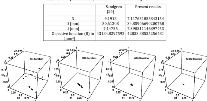
Table 3. Comparison of optimal results – discrete real and integer design variables. Sandgren
[54] Wu, Chow [55] resultsPresent
N 10 9 9
D [mm] 29.9898054 31.176239431.06544712 d [mm] 7.1882=0.283[inch] 7.1882 7.1882 Objective function (8)
[mm3] 45547.844388 43722.3254643565.99925
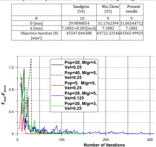
0 100 200 300
Number of Iterations
0 0.4 0.8 1.2
Fbe
st
-Fw
or
st
Pop=20, Migr=5, Vel=0.25
Pop=40, Migr=5, Vel=0.25
Pop=5, Migr=5, Vel=0.25
Pop=20, Migr=5, Vel=0.125 Pop=20, Migr=3, Vel=0.25
Figure 5. Convergence of numerical computations – the accepted error equals to 10-7.
Although, as it is proved above, the proposed evolution strategy allows us to obtain very good, even excellent numerical results it is necessary to mention about the influence and the role of strategy parameters, i.e. the total number of individuals in the population (pop), the velocity of the strategy (vel) and the number of migrations (migr). They can affect significantly the convergence as well as the efficiency of the optimization algorithm since they have a great influence on the so-called oscillations of solutions – visible also in Fig.5. When vel is very high it hits the boundary on nearly every iteration and this ineffective trajectory searches the same points repeatedly. As
vel is low the particle explores the optimum very slowly – see Fig.4. Reducing the number of migrations one can observe the similar effect as previously, i.e. the efficiency of the numerical process decreases. The growth of the number of population (pop) also increases the number of iterations required for searching for the optimum with the prescribed value of accepted error. However, on the other hand, the increase of the pop parameter is necessary in the verification of the location of the global optimum.
B. Cylindrical Panel with Discrete Fibre Orientations
2 2
33 23 11 23 12 13 13 12 23 22 13 11 22 12
2 2 3 2 2 2
11 11 66 12 12 66 13 12 11 12 66 22 22 66
2 3
23 12 66 22 22
/ , / , /
, ( ) , / 2 , ,
2 / ,
xcr m m n
m n m n m m m n n m
m n n n
P K K K K K K K K K K K K K K m L n R
K A A K A A K A R B B B K A A
K B B A R B
4
2 2 4
2 2
33 11 m 2 12 2 66 m n 22 n 22/ 2 22 n 2 12 m / ,
K D D D D A R B B R
(17)
Assuming the mid-plane symmetric case (Bij=0) the critical pressure can be expressed as the sum of two
terms:
2 4 2 2 4
11
2
122
66 22xcr m m m n n rs
P
D
D
D
D
s A
,
2
2
11 22 122
66
2 4 2 2 2 4
11 66 11 22 12 2 12 66 22 66
m m
rs
m m n n
A A A A s A
R A A A A A A A A A
(18)
Assuming that the term s in Eq. (18) is identically equal to zero the relation (18) is analogous to the buckling relation for rectangular plates if the meridional coordinate is designated x, and the circumferential y, whereas the left hand in Eq. (18) can be replaced by the formulae:
2 2
2n y m
x P
P representing the bi-axial compressive forces Px and Py.
For isotropic cylindrical shells the buckling load (18) is reduced to the following form – Eq. (19):
2 2 2
2 2
1 ,
,
12 1
m n xcr mR
Et
t
P
AS
AS
R
AS
(19)what means that the second term (membrane) in Eq. (3), denoted by the symbol s, plays a significant role. It is seen that the critical load is a function of geometrical ratios t/R and L/R. For isotropic shells to find the optimal buckling force let us assume that the derivative of Pxcr with respect to L is equal to zero and the corresponding
minimum buckling load – Eq. (20) is:
2
/
3 1
xcr
P
Et R
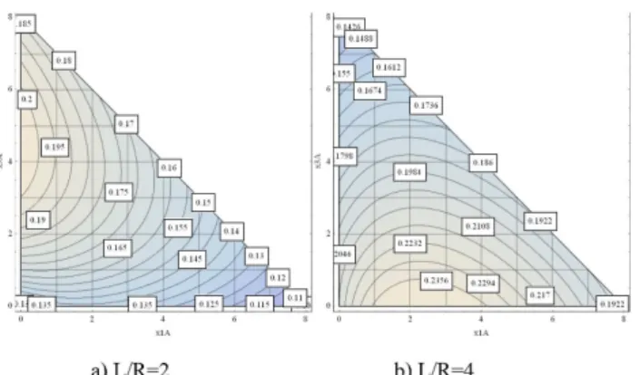
(20)For composites the relation between the bending and membrane states depends not only on the values of the geometrical ratios t/R and L/R, but also on the mechanical properties and laminate configurations. Therefore, the identical procedure to that mentioned for isotropic structures cannot be conducted. It is seen in Figs 6 a, b. For the discrete fibre orientations 00, ±450, 900 in the laminate let us use the design variables in the form of four integers
{x1A ,x3A,x1D ,x3D} defined by Muc [56].
The optimization problem (Eqs (21), (22)) is defined as follows. To find:
1A, , ,3A D1 3D xcr
x x x x
Min P
(21)subjected to six constraints:
1A
, , ,
3A 1D 3D1,
1A 3A1,
1D 3D1
x x x x
x
x
x
x
(22)Figure 6. The positions of the optimal buckling loads for three discrete fibre orientations (m=n=1, membrane state only – the function s in Eq.(18))
The bending part of Eq. (18) can be expressed as the linear function of two variables x1D ,x3D in the following form – Eq. (23):
2 2 3
1 2 1D 3 3D
/12
x m
P
t Z Z x
Z x
(23)where Z1, Z2 and Z3 are constants in the optimization problem. Since the constants are positive the maxima always
occurs at the boundaries (x1D0 or x3D0). It is worth to emphasize that the contour plot solution gives directly the number of plies having orientations 00, ±450, 900 but not their location in the laminate. The location of those
plies can be found by the analysis of the values x1D ,x3D. However, having an information about the positions of the optimal stacking sequences for bending states it is possible to find independently the positions of maximal buckling loads (the optimal stacking sequence) for membrane states only, and then to join the results. With the use of the decoding procedure is possible to find a series of the corresponding to values x1A ,x3A the values x1D ,x3D and to calculate the value of the bending term (23).
C. Buckling of Cylindrical Shells with Domed Heads
In engineering constructions composite cylindrical shells are closed by domed heads having various forms as: flat plates, ellipsoidal, torispherical, spherical, paraboloidal or even conical. We intend to analyse the influence heads on buckling loads and forms. The presented analysis is a parametric study of various geometrical effects and it is treated as an introduction to optimal design in the form similar to that studied by Muc [53]. In the present optimal design we tend to minimize the geometrical ratio L/D where the value of the buckling external pressure (pbuckl) does not exceed the allowable value of the pressure (pallow) – Eq. (24), i.e.:
buckl allow
p
p
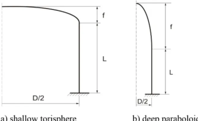
(24)In particular the considerations deal with composite pressure vessels having the domed heads in the form of: a) shallow torisphere (R/D=1, r/D=0.1) with a cylindrical part – Figure 7a, b) deep paraboloid (f/D=1.5, i.e. z=6r2/D) with a cylindrical part – Figure 7b. It is assumed that the shells are made of carbon/epoxy resin and
have quasi-isotropic material properties. The numerical investigations are carried out for axi-symmetric structures taking into account geometrical pre-buckling nonlinearities. The results of buckling investigations for spherical and ellipsoidal domes were studied by Muc [54,55].
Figure 7. Forms of the analysed pressure vessels with domed heads
Figure 8. The effects of the cylindrical part length on the buckling loads
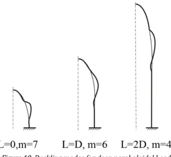
Figs 9, 10 demonstrate buckling modes for various lengths of the cylindrical part starting from L/D=0. As it may be seen the buckling mode (the number m) is also dependent on the L/D ratio. In general, it is reduced with the growth of the geometrical L/D ratio.
The results of buckling investigations for spherical and ellipsoidal domes with and without cylindrical portions and the possibility of optimal design were studied in details by Muc [57,58].
Figure 10. Buckling modes for deep paraboloidal heads
D. First-Ply-Failure of Laminated Plates with Holes
For a infinite laminated plates subjected to axial/biaxial compression/tension or in-plane shear and having a circular/ elliptical hole the optimum design of laminate stacking sequence is presented by Sharma et al. [59]. The authors of the paper adapted the formulation and the solution given by Lekhnitski [60], Savin [61] for stresses around holes in an infinite angle-ply balanced symmetric laminated plates under in-plane loading (Fig.1) – Eq. (25):
4 2
11
2(
12 66)
220
T s
T
T s T
(25)Tij represent the classical terms of the compliance matrix for the plane stress problem.
Figure 11 Laminated plate containing an elliptical opening where θ denotes the (ith) ply orientation
The solutions sj of the above characteristic equation are represented by the complex numbers – see e.g. Muc,
0 1 2
2 2 2
1 2 1 2
1 2 0
2 2 2
1 2 1 2
0 1 2
2 2 2
1 2 1 2
cos
Re
sin
sin cos
cos
cos
sin
1 Re
sin
sin cos
cos
sin cos
Re
sin
sin cos
cos
i x i y i xy
N
e
s s
t
d s s
d s s
d s s
N
e
t
d s s
d s s
N
e
ds s
t
d s s
d s s
,1/
d a b
/
(26)
where α is the angular coordinate measured along the ellipse from the axis 0-x, (σy=σ∞ =N0/t at the direction y –
Fig.11), and s1, s2 are the complex roots of the equation (25). For orthotropic or cross-ply structures the roots can
be expressed by the relations (27):
21,2
4
/ 2,
/
2
4
s
Delt i Delt
E
Delt
E G
E
(27)where:
11 66
11 12
2
22 11 22 12 22
,
A A
,
A
A
E
G
A
A A
A
A
and Aij denote the in plane stiffness of the laminate.
In an infinite orthotropic plate the analytical solution for the stress component σy at the edge of a hole and
α=00 is given by Eq. (28):
0
0
1 2
1 20
1 Re
y
i s s
N
t
ds s
(28)However, the above relations cannot be used in the optimization analysis since for finite width of the plate the stress distributions/concentrations around the holes are different than those compared with the results for infinite plates. It was demonstrated by Muc, Ulatowska [62] and Xu Xiwu et al. [63]. Tan [64] introduced the approximate formulas for the stress concentration factors for the orthotropic laminated plates valid in the range 0≤b/a≤1 – Eq. (29):
2 2
2
2 2 2
2
7 3 5/2 7/2
2 2
1 2
1
1
1
1
1
1
1
2
2
1
1
1
1
1
,
2
t
tg
t
x
K
d
d
d
d
K
d
d
d
d
d
K
d
d
a
d
L
(29)where Kt∞ is the stress concentration factor for the infinite plate that can be derived from the following formula
(30):
2 11 22 12 11 22 12
66 66
1
2
1
2
t
A A
A
K
A A
A
d A
A
(30)and Aij denotes the effective laminate in-plane stiffnesses with 1 and 2 corresponding to parallel and
perpendicular to the loading directions (Fig.11), i.e. to the y and x directions, respectively.
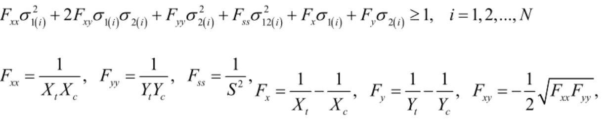
The optimization problem is formulated in the following way: to maximize the tensile load – Eq. (31), i.e.: 0
Max N
(31)
2 2 2
1
2
1 2 2 12 1 21, 1,2,...,
xx i xy i i yy i ss i x i y i
F
F
F
F
F
F
i
N
(32)2
1
,
1
,
1
,
1
1
,
1 1
,
1
,
2
xx yy ss
t c t c x y xy xx yy
t c t c
F
F
F
X X
YY
S F
F
F
F F
X
X
Y Y
The constraints represent the First-Ply-Failure (FPF) in the form proposed by Tsai-Wu. The criterion is formulated in the local coordinate system (1-2) defined previously. Xt, Xc, Yt, Yc are allowable stresses for tension
(t), compression (c) in the directions parallel (X) and perpendicular (Y) to fibres, and S denotes the allowable in-plane shear stresses. For each of the plies the transformation rule between the local (1-2) and the global coordinate system is defined by Eq. (33) below. The transformation is valid for the (ith) ply, however the symbol (i) is omitted.
2 2
1 2 2
2 3 4 5
2 2
12
cos
sin
0
0
0
sin 2
sin
cos
0
0
0
sin 2
0
0
1
0
0
0
0
0
0 cos
sin
0
0
0
0 sin
cos
0
1
sin 2
1
sin 2
0
0
0
cos
sin
2
2
xx
yy
zz
yz
xz
xy
, (33)
Similarly as in the previous section for the assumed discrete fibre orientations 00, ±450, 900 in the laminate
let us use the design variables in the form of two integers
x x
1A,
3A
- the behaviour of the laminate is characterized by the in-plane laminate coefficients Aij. In addition, for the comparison of the results, the angle-ply(±θ) symmetric laminate stacking sequence is considered.
In the numerical finite element analysis the following values of the material constants are assumed: E1=46.43 [GPa], E2=14.9 [GPa], G12=5.233 [GPa], ν12=0.269, Xt=Xc=1534 [MPa], Yt=Yc=74.5 [MPa], S= 115 [GPa].
They corresponds to glass fibre/epoxy composites.
The failure strength for the angle-ply laminate was calculated varying the ply orientations in the interval [0,90]. The optimal fibre orientations corresponding to the maximal failure loads are given below:
− Circular hole – θ=30 − Vertical elliptical hole - θ=0 − Horizontal elliptical hole - θ=38
It was found that the increase of the curvature resulted in the increase of the maximal failure strength, i.e. the highest failure strength was observed for the horizontal ellipses and the lowest for the vertical elliptical holes. The obtained optimal fibre orientations presented by Sharma et al [59] are different than those presented above since the mentioned authors analysed infinite plates only.
For discrete fibre orientations the distributions of the strength were analysed in the triangular space of design variables. The results are plotted in Fig. 12 for circular hole. The maximum of the strength occurred for fibres oriented at 0 (8 plies) and 90 (8 plies). The plies oriented at 45 were not present in the optimal stacking sequence. The sequence of the plies oriented at 0 and 90 is not important in the analysis since the values of the terms Aij do not vary with the change of the stacking sequences.
For laminated multilayered plates with a cut-out more information about the stress concentration problems can be found in Refs [65-67].
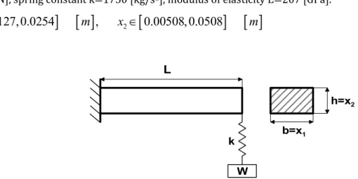
E. Vibration Frequency of the Cantilever Beam-Mass System
Let us consider the cantilever beam system shown in Fig.13. The beam cross section is rectangular. The objective function is to find the optimal cross-sectional dimensions a and b that minimize the weight of the beam (the beam length is constant) while keeping the fundamental vibration frequency larger than 8 rad/sec. Thus, the fundamental optimization problem can be represented by Eqs (34)-(38):
1 2
Min x x
(34)subjected to the constraint:
8
/ sec
e
k
rad
m
(35)where:
3 3
1 2
1
1
,
,
,
3
12
e
x x
L
I
m
W
k
k
EI
g
(36)and gravitational constant g=9.81 m/s2, length of the beam L=0.381 [m], weight attached to the spring
W=267 [N], spring constant k=1750 [kg/s2], modulus of elasticity E=207 [GPa].
1
0.0127,0.0254
,
20.00508,0.0508
x
m
x
m
(37)L
b=x1
h=x2
W k
Figure 13. The cantilever beam-mass system
The analytical solution of that problems exists and the optimum can be found at the boundary:
3 3
1 1 2 1 2
1
4
0.5,
1.2,
0.6
64
1
L
L
k L E
x x
x
Area x x
x k
m
0 0.1 0.2 0.3 0.4 0.5 0.6 0.7 0.8 0.9 1 0
0.1 0.2 0.3 0.4 0.5 0.6 0.7 0.8 0.9 1
1 Generation
0 0.1 0.2 0.3 0.4 0.5 0.6 0.7 0.8 0.9 1 0
0.1 0.2 0.3 0.4 0.5 0.6 0.7 0.8 0.9 1
5 Generation
0 0.1 0.2 0.3 0.4 0.5 0.6 0.7 0.8 0.9 1 0
0.1 0.2 0.3 0.4 0.5 0.6 0.7 0.8 0.9 1
20 Generation 0 0.1 0.2 0.350 Generation0.4 0.5 0.6 0.7 0.8 0.9 1
0 0.2 0.4 0.6 0.8 1
0.1 0.3 0.5 0.7 0.9
Figure 14. Convergence of the numerical algorithm – pop=10, vel=0.3, migr=5 (dimensionless variables)
The use of the proposed optimization algorithm allows us to obtain the identical results as above very quickly, after 50 generations with the error ε equals to 10-7. For different number of generations numerical results
are plotted in Fig.14 – dimensionless design variables. As it may be seen they present an excellent convergence and accuracy.
F. Optimal Proportion of the I-shaped Cross Section
A lot of modern sheet isotropic or composite constructions require stiffeners that are normally of I-, Z- or C-shaped cross sections. An I-C-shaped cross section, shown in Fig. 15, has been selected in our example. Since a large number of these stiffeners are employed, it is important to find the optimal proportion of its dimensions x1, x2 and
x3 being design variables in our problem. A stiffener is treated as an axially loaded column, as shown in Fig. 15.
The goal is to have a minimal volume of the the column (understood in the sense of the area A since the column length L is constant):
2
1 2(
32 )
1 1
MinA
Min x x
x
x x
(39)while meeting the following yield stress and buckling conditions: yield stress:
y
A /
P (40)
x1=t
x2=b
x3=h
x y
2 min
min
2
,
( , ),
x yEI
P
I
Min I I
L
(41)
3 2 3 3 3
1 1 1 1 1
2 1 1 2 3 1 1 3 1 1 2 1 3 1
6 2
(
)
12(
2 ) ,
6 12(
2 )
x y
I
x x
x x x x
x x
x
I
x x
x x
x
, (42)flange buckling load: 2 2
1 2
2
2
0.43
12(1
)
x
E
A P
x
, (43)web buckling load: 2 2
1 2
3
4
12(1
)
x
E
A P
x
, (44)applied load P=8.9 [kN], yield stress
y=172.4 [MPa], Young's modulus E=69 [GPa], Poisson's ratio ν=0.3, length of stiffener L, and:
1
0.00254,0.0076 2 [ ],
20.00508,0.0762 [ ],
30.01016,0.1016 [ ]
x
m
x
m
x
m
(45)L P
Figure 15. The axially loaded column having the I-shaped cross-section
Table 4. Optimal dimensions of the I cross section.
L [mm] A [mm2] t [mm] b [mm] h [mm]
254 76.6506 2.54 12.5487 10.16
508 123.364 2.54 19.9514 13.7456
1651 278.25 2.54 43.8142 26.9987
2032 364.659 2.80606 48.6718 38.2228
500 1000 1500 2000 2500
L [mm] 0
100 200 300
A - area [mm^2] t - thickness [mm] b - width [mm] h - height [mm]
Figure 16. Variations of the optimal cross-section dimensions (pop=25, vel=0.3, migr=5)
VI. Concluding Remarks
The present review of existing works in the open literature demonstrates evidently that the number of results rapidly increases without the proper comparison of them. Therefore, it is practically impossible to draw more general conclusions even in the specific area of interest. Although, the number of references in each of the papers also grows it is very difficult to track and compare the validity of the published results in view of various assumptions made in different works. Such a situation may lead to misunderstanding and pitfalls for researchers.
We do not intend to discuss herein the problem of the choice of the design variables (see Ref[68].). However, the investigations are mainly focused on the assumptions that may affect significantly on the results and then on the comparison of results.
The detailed analysis demonstrated evidently that the proposed algorithm works well for different optimization problems, various number of design variables and equality or inequality constraints. More information about those problems can be also found in Ref [53].
also for multilayered composite structures. The effectiveness of the algorithm is strongly dependent on the proper choice of the evolution strategy parameters.
Acknowledgment
The research project has been financed by National Science Center Poland pursuant to the decision No.DEC-2013/09/B/ST8/00178.
References
[1] H. Wilf, Algorithms and Complexity, Second Edition, A. K. Peters Ltd, Wellesley, MA, 2002.
[2] W. J. Cook, W. H. Cunnigham, W. R. Pulleyblanh, A. Schriveer., Combinatorial Optimization, John Wiley & Sons, New York-Chichester-Weinheim-Brisbane-Singapore-Toronto, 1997.
[3] R.Haftka, Z.Gurdal, Elements of Structural Optimization, Kluwer Academic Publisher, Dordrecht, 1993.
[4] M. Dorigo, M. Birattari, and T. Stutzle, „Ant colony optimization”, IEEE Computational Intelligence Magazine, vol.1,pp.28-39, 2006.
[5] Wenjun Pan and L. P. Wang, “An Ant Colony Optimization Algorithm Based on the Experience Model”, Proc. 5th International Conference on Natural Computation (ICNC 09), 2009.
[6] Bifan Li, L. P. Wang and Song Wu, “Ant colony optimization for the travelling salesman problem based on ants with memory”, Proc. 4th International Conference on Natural Computation (ICNC 08), vol.7, pp.496-501, 2008. [7] M. Dorigo and C. Blum, “Antcolony optimization theory: A survey”; Theoretical Computer Science, vol.344, pp.243-278, 2005.
[8] M. Dorigo, T.Stutzle, T., Ant Colony Optimization, MIT Press, Cambridge-Massachusetts, London-England, 2004. [9] L. Castro, J. Timmis, “An Artificial Immune Network for Multimodal Function Optimization” Proc.IEEE Congr. Evolut. Comp. (CEC'02), vol. 1, pp. 699-674, 2002.
[10] P. Moscato, “Memetic algorithms: A short introduction” In New Ideas in Optimization, D. Corne et al. (eds) McGraw-Hill, UK Maidenhead, UK England, pp. 219-234,1999.
[11] F. Glover, “Heuristics for Integer Programming Using Surrogate Constraints,” Decision Sciences, vol. 8, pp. 156-166, 1977.
[12] F. Glover, “Tabu Search for Nonlinear and Parametric Optimization (with Links to Genetic Algorithms),”
Discrete Applied Mathematics, vol. 49, pp. 231-255, 1994.
[13] R. Eberhart, J. Kennedy, “A New Optimizer Using Particle Swarm Theory”; MHS 95: Proc. 6th Int.Symp. Micro Mach.&Human Sc., 1995.
[14] L. P. Wang, Guanglin Si, “Optimal location management in mobile computing with hybrid genetic algorithm and particle swarm optimization (PSO)”, IEEE Int. Conf. on Electronics, Circuits & Systems (ICECS 2010), Greece, 2010.
[15] Xiuju Fu, Sonja Lim, L. P. Wang, Gary Lee, Stefan Ma, Limsoon Wong, Gaoxi Xiao, “Key node selection for containing infectious disease spread using particle swarm optimization”; IEEE Swarm Intelligence Symposium (SIS 09), 2009.
[16] J. Kennedy, “Particle Swarm Optimization”,in Encyclopedia of Machine Learning, pp 760-766, 2010.
[17] J. McCall, “Genetic algorithms for modelling and optimisation”, J.Comp.Appl. Math., vol.184, pp.205-222, 2005. [18] L. P. Wang, Sa Li, Sokwei Cindy Lay, Wen Hsin Yu, and Chunru Wan, “Genetic algorithms for optimal channel assignments in mobile communications,” Neural Network World, vol.12, pp. 599-619, 2002.
[19] X.J. Fu and L.P. Wang, “Rule extraction by genetic algorithms based on a simplified RBF neural network”, Proc. 2001 Congress on Evolutionary Computation, pp.753-758, 2001.
[21] Sa Li, Sokwei Cindy Lay, Wen Hsin Yu, and L. P. Wang, “Minimizing interference in mobile communications using genetic algorithms”, Proc. Int. Conf.Comp.Sc. (ICCS 2002), vol. I, pp. 960-969, LNCS 2329, 2002.
[22] I. Jawahar and J. Wu. “A Two Level Random Search Protocol for Peer-to Peer Networks”. In Proc. 8th world Multi-Conf. Systemics, Cybernatics and Informatics, 2004.
[23] S. Kirkpatrick, C. D. Gelatt, M. P. Vecchi, “Optimization by Simulated Annealing”; Science, vol.220, No.4598, pp.671-680, 1983.
[24] L. P. Wang, N. S. L. Sally, W. Y. Hing, “Solving channel assignment problems using local search methods and simulated annealing”, Independent Component Analyses, Wavelets, Neural Networks, Biosystems, and Nanoengineering IX, vol.8058, a part of SPIE Defense, Security, and Sensing, 25-29 April 2011, Orlando, Florida, USA.
[25] R.W. Eglese, “Simulated annealing: A tool for operational research”; Europ. J. Operational Research, vol.46, pp.271-281, 1990.
[26] Motwani, Rajeev; Raghavan, Prabhakar, Randomized Algorithms. New York: Cambridge University Press, 1995.
[27] F. Larumbe and B. Sanso, “A Tabu Search Algorithm for the Location of Data Centers and Software Components in Green Cloud Computing Networks”, IEEE Trans. Cloud Computing, vol.1, pp.22-35, 2013.
[28] Yanjie Peng, Boon Hee Soong, and L.P. Wang, “Broadcast scheduling in packet radio networks using mixed tabu-greedy algorithm”, Electronics Letts., vol.40, pp.375-376, 2004.
[29] G. Cavuslar, B. Catay, and M.S. Apaydin, “A Tabu Search Approach for the NMR Protein Structure-Based Assignment Problem”; IEEE-ACM Trans. Comp. Biology and Bioinformatics, vol.9, pp.1621-1628, 2012.
[30] J. Hoffmann, and B. Nebel, “The FF planning system: Fast plan generation through heuristic saearch”. J. Artificial Intelligence Research, Vol. 14, 253–302.2001.
[31] H. Nozawa, “A Neural-Network Model as a Globally Coupled Map and Applications Based on Chaos,” Chaos, vol. 2, pp. 377-386, 1992.
[32] L.N. Chen and K. Aihara, “Chaotic Simulated Annealing by a Neural Network Model with Transient Chaos,” Neural Networks, vol. 8, pp. 915-930, 1995.
[33] L.P. Wang, Wen Liu, and Haixiang Shi, “Delay-constrained multicast routing using the noisy chaotic neural networks,” IEEE Trans. Computers, vol.58, pp.82-89, 2009.
[34] L.P. Wang, Wen Liu, and Haixiang Shi, “Noisy chaotic neural networks with variable thresholds for the frequency assignment problem in satellite communications,” IEEE Trans. System, Man, Cybern, Part C-Reviews and Applications, vol.38, pp.209-217, March, 2008.
[35] L. P. Wang and Haixiang Shi, “A gradual noisy chaotic neural network for solving the broadcast scheduling problem in packet radio networks,”IEEE Trans. Neural Networks, vol.17, pp.989-1000, 2006.
[36] L. P. Wang, Sa Li, Fuyu Tian, and Xiuju Fu, “A noisy chaotic neural network for solving combinatorial optimization problems: Stochastic chaotic simulated annealing", IEEE Trans. Systems, Man, Cybern, Part B-Cybernetics, vol.34, pp.2119-2125, 2004.
[37] P. Siarry and Z. Michalewicz (Edts), Advances in Metaheuristics for Hard Optimization, Springer-Verlag, Berlin-Heidelberg 2008.
[38] D.H. Wolpert, W.G. Macready, No free lunch theorems for optimization, IEEE Trans. Evolutionary Computations, vol. 1, 1997, pp. 67-82.
[39] A. Muc, Transverse shear effects in discrete optimization of laminated compressed cylindrical shells,
Composite Structures, vol. 38, 1997, ss. 211-22.
[40] A. Muc, W. Gurba, Genetic algorithms and finite element analysis in optimization of composite structures,
Composite Structures, vol. 54, 2001, ss. 275-81.
[43] IEEE Neural Network Council, Glossary of Evolutionary Computations Terms (Working Draft), Standing Committee on Standards, IEEE, Piscatway,NJ, 1996.
[44] A. S. Fraser, Simulation of genetic systems by automatic digital computers, Australian Journal of Biological Science, vol. 10, 1957, pp. 484-499.
[45] J. H. Holland, Outline for a logical theory of adaptive systems, Journal of the Association for Computing Machinery, vol. 3, 1962, pp.297-314.
[46] L.J. Fogel, A.J. Owens, M.J. Walsh, Artificial Intelligence through Simulated Evolution, 1966, New York, John Wiley & Sons.
[47] I. Rechenberg, Cybernetic solution path of an experimental problem, Royal Aircraft Establishment, Library Translation 1122, Farnborough, Hants, U.K., 1965.
[48] H.P. Schwefel, Kybernetische Evolution als Strategie der experimentallen Forschung in der Stromungstechnik,
Diploma Thesis, Technical University of Berlin, 1965.
[49] R.M. Friedberg, A learning machine: Part I. IBM Journal of Research and Development, Vol. 2, 1958, pp.2-13. [50] I. Rechenberg, Evolution strategy, In J. Zurada, R. Marks II, and C. Robinson (Eds.), Computational Intelligence-Imitating Life, Piscataway, NJ:IEEE Press, 1994, pp.147-159.
[51] A.E.Eiben, J.E. Smith, Introduction to Evolutionary Computing, Springer-Verlag, Berlin, 2003.
[52] J.R. Koza, Genetic Programming: On the Programming of Computers by Means of Natural Selection, Cambridge, MA: The MIT Press, 1992.
[53] A. Muc, and M. Muc-Wierzgoń, An evolution strategy in structural optimization problems for plates and shells, Composite Structures 94 (4), 2012, pp. 1461-1470.
[54] E. Sandgren, Nonlinear integer and discrete programming in mechanical design optimization, ASME Trans., J. Mech. Design, 112, 1990, pp. 223-229.
[55] S.-J. Wu, P.-T. Chow, Genetic algorithms for nonlinear mixed discrete-integer optimization problems via meta-genetic parameter optimization, Engineering Optimization, 24, 1995, pp. 137-159.
[56] Muc A. 2004, “An evolution strategy in optimal design of composite structures”, Collection of Technical Papers - 10th AIAA/ISSMO Multidisciplinary Analysis and Optimization Conference 2, pp. 1023–1031.
[57] A. Muc, 1991, “Buckling and postbuckling behaviour of imperfect laminated shallow spherical shells under external pressure”, Composite Structures - VI, London, pp. 281-296.
[58] A. Muc, 1991, “Buckling analysis of laminated ellipsoidal shells subjected to external pressure”, Composite Structures - VI, London, pp. 298-314.
[59] Sharma, D.A., Patel, N.P., Trivedi, R.R., Optimum design of laminates containing an elliptical hole, International Journal of Mechanical Sciences 85 (2014) 76–87
[60] Lekhnitskii S. G. Anisotropic plates. New York: Gordon and Breach, 1968. [61] Savin G.N. Stress concentration around holes. New York:Pergamon Press, 1961.
[62] S.C. Tan, Laminated composites containing elliptical opening, J. Comp. Mater. 21 (1987) 925-948.
[63] A. Muc., A. Ulatowska, Local fibre reinforcement of holes in composite multilayered plates, Composite Structures 94 (2012), 1413-1419
[64] Xu Xiwu, Sun Liangxin, Fan Xuqi, Stress Concentration of Finite Composite Laminates with Elliptical Holes, Computers & Stuctures 57 (1995), 29-34.
[65] A Muc, P Romanowicz, Effect of notch on static and fatigue performance of multilayered composite structures under tensile loads, Composite Structures, 2017, 178, 27-36
[66] A Muc, M Barski, M Chwał, P Romanowicz, A Stawiarski, Fatigue damage growth monitoring for composite structures with holes, Composite Structures, 2018, 189, 117-126