Hydrodynamic Modelling of Ria Formosa (South Coast of Portugal) with EcoDynamo

Hydrodynamic Modelling of Ria Formosa (South

Coast of Portugal) with EcoDynamo

Pedro Duarte, Bruno Azevedo and António

Pereira

University Fernando Pessoa, Centre for

Modelling and Analysis of Environmental

Systems

DITTY (Development of an information technology tool for the

management of Southern European lagoons under the influence of

river-basin runoff)

(EESD Project EVK3-CT-2002-00084)

Summary

In this work a hydrodynamic model of Ria Formosa (South of Portugal) is

presented. Ria Formosa is a large (c.a. 100 km2) mesotidal lagunary system

with large intertidal areas and several conflicting uses, such as fisheries,

aquaculture, tourism and nature conservation. This coastal ecosystem is a

natural park where several management plans and administrative

responsibilities overlap.

CONTENTS

1 Introduction ... 1

1.1 Site description ... 1

1.2 Objectives ... 2

2 Methodology... 3

2.1 Model description... 3

2.2 Model implementation... 10

2.3 Model calibration and validation...11

2.4 Analysis of general circulation patterns and residence times... 13

2.5 Dilution of effluents from Waste Water Treatment Plants... 13

3 Results and Discussion ... 15

3.1 Model calibration and validation... 15

3.2 Analysis of general circulation patterns and residence times... 22

Fig. 3-20 – Half residence time (a) and time for 90% washout (b) of eastern lagoon water (see text)... 29

3.3 Dilution of effluents from Waste Water Treatment Plants... 30

4 Conclusions ... 36

1 Introduction

This work is part of the DITTY project “Development of an Information Technology Tool for the Management of European Southern Lagoons under the influence of river-basin runoff” (http://www.dittyproject.org/). The general objective of this project is the development of information technology tools integrating Databases, Geographical Information Systems (GIS), Mathematical Models and Decision Support Systems to help in the management of southern European coastal lagoons and adjacent watersheds, within the spirit of the Water Framework Directive (UE, 2000).

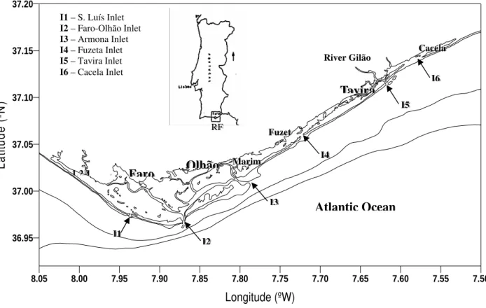
The DITTY project takes place in five southern European coastal lagoons. The work presented here concerns the hydrodynamic modelling of Ria Formosa – the Portuguese case study within DITTY (Fig. 1-1). The coupling of this model with a biogeochemical model including water and sediment processes will be the subject of an upcoming report.

1.1 Site description

Figure 1-1- Geographic location of Ria Formosa and its inlets (I1 – I6).

1.2 Objectives

The objectives of this report are to:

i. Describe the model and how it was implemented, giving details on numerical methods and software developed

ii. Describe model calibration and validation

iii. Use the model to analyse general circulation patterns and estimate water residence times

iv. Use the model to analyse the dispersion of effluents rejected by the Waste Water Treatment Plants (WWTP) located in Ria Formosa.

8.05 8.00 7.95 7.90 7.85 7.80 7.75 7.70 7.65 7.60 7.55 7.50

Longitude (ºW) 36.95 37.00 37.05 37.10 37.15 37.20 L a ti tu d e ( ºN ) I

II111

I

II222

A AAtttlllaaannntttiiiccc

I

II333

I

II444

I

II555 I

II666

I1 – S. Luís Inlet

I2 – Faro-Olhão Inlet I3 – Armona Inlet

I4 – Fuzeta Inlet I5 – Tavira Inlet

I6 – Cacela Inlet

F

FFaaarrrooo OOOlllhhhãããooo

T TTaaavvviiirrraaa

M

MMaaarrriiimmm

C

CCaaaccceeelllaaa

1.2.1 A

R RRFFF

F

FFuuuzzzeeettt

Atlantic Ocean

2 Methodology

2.1 Model description

The hydrodynamic model implemented in this work is a two dimensional solution of the Navier-Stocks equations adapted from Neves (1985). It is based on a finite difference staggered grid (Vreugdenhil, 1989). Flows are solved at the sides of the grid cells, whereas surface elevations and concentrations are calculated at the center of the cells. Advection terms are calculated using an upwind scheme, whereas diffusion terms are based on a central differences scheme (see below). The resolution is semi-implicit. At the first semi time step the u component is solved implicitly and the vcomponent solved explicitly. At the second semi time step it is the other way around. After the calculation of both velocity components, surface elevation is calculated by continuity, as well as the concentration of conservative and non-conservative substances, after solving for the sources and sinks. The model is forced by tidal height at the sea boundaries. It can also be forced by wind and fresh water flows.

Equation of Continuity

(

)

(

)

(

)

(

)

+

+ + + − + + −

ξ − ξ

+ + − + +

∆ ∆

+ − + =

∆ 1 n

n 1

2 _n

ij ij ₂

IJ IJ 1 ij 1 ij ij 1 ij

n ij i 1j i 1j ij i 1j ij

1

H H u H H u

t / 2 2 x 1

H H v H H v 0

2 x

(1)

ξ- Surface elevation (m)

∆x- Spatial step (100 m) H- Depth (m)

u and v - Current speed (East-West and North- South, respectively) (m s-1)

nand n+1

At the second semi time step the u terms are reported to time n+1

2 and the v terms are

reported to time n.

Equation for the u component at the first semi time step

The second and third terms on the left side of the equation are the advection components, the first term on the right side is the barotropic pressure gradient acceleration, the second term corresponds to drag, the third term is the Coriolis acceleration and the fourth term corresponds to momentum transfer by diffusion.

1 n ₂

ij ij 1 ij 1 ij ij 1 ij 1 ij 1 ij 1

2 2 2 2

1

n _{2 n}

ij ij

ij ij 1

ij _ij 1 _ij 1 ij 1 ij 1 _ij 1 _ij 1 ij

2 2 2 2

1 1 1 1

i j i j

2 2 2 2

ij ij 1

H u u u H u u u

u u 1 _{x x}

t / 2 (H H )

H u u u H u u u

x x

H v

1 (H H )

+ − − + + − − + − + − + + − − + − + − − + + − + − _{∆ ∆} + + ∆ + _{− −} − ∆ ∆ + + n

1 1 ij 1 1 1 1 1 1 i 1j

i j i j i j i j

2 2 2 2 2 2 2 2

1 1 1 1 1 1 i 1j 1 1 1 1 1 1 ij

i j i j i j i j i j i j

2 2 2 2 2 2 2 2 2 2 2 2

v u H v v u

x x

H v v u H v v u

x x − + − − − − − − − + + − + − + − − − − − − − + + − + ∆ ∆ ₌ − − − ∆ ∆ 1 1 n n

2 2 ₁

n

ij ij 1 ₂

ij ij 1 ij ij ij 1

1 n

2 ij 1 ij 1 i 1j 1 i 1j

1

n _{2 n}

ij 1 ij 1 ij i 1j i 1j ij

2

1

g (Cf Cf ) u u

x (H H )

1

f(v v v v )

4

(u u 2u ) (u u 2u )

x + + + − − − + − − + − + + + − + −

ξ − ξ

= − − + +

∆ +

+ + + +

ν _{+ − + + −}

∆

(2)

Where,

g - Acceleration of gravity (m s-2)

Equation for the v component at the first semi time step

All terms are presented in the same order as for the ucomponent (see above).

n

ij _i 1 _{j i} 1 _j ij i 1j _i 1 _{j i} 1 _j i 1j

2 2 2 2

1

n _{2 n}

ij ij

ij i 1j

ij _i 1 _{j i} 1 _j i 1j i 1j _i 1 _{j i} 1 _j ij

2 2 2 2

n

1 1 1 1

i j i j i

2 2 2 2

ij i 1j

H v v v H v v v

t x x

v v

2(H H )

H v v v H v v v

x x

H u u

t 2(H H )

− − + + − − + − + − + + − − − + − + − + + − + ∆ _{∆ ∆} = − − + _{− −} − ∆ ∆ + ∆ +

1 j 1 ij i 1 j 1 i 1 j 1 i 1 j 1 ij 1

2 2 2 2 2 2 2 2

1 1 1 1 1 1 ij 1 1 1 1 1 1 1 ij

i j i j i j i j i j i j

2 2 2 2 2 2 2 2 2 2 2 2

n n

ij i 1j

ij i ij i 1j

v H u u v

x x

H u u v H u u v

x x

t t

g (Cf Cf

2 x 2(H H )

− − + − − − − − − + − + − + − + − − − − − − − − + − − ∆ ∆ ₋ − − − ∆ ∆

ξ − ξ

∆ ₋ ∆ ₊

∆ +

n

1j ij ij ij 1 i 1j i 1j 1

n n

ij 1 ij 1 ij i 1j i 1j ij

2

t

) v v f(u u u u )

8

t

(v v 2v ) (v v 2v )

2 x − + − − + + − + − ∆ + + + + +

ν∆ _{+ − + + −}

∆

(2)

Equation 1 is used to substitute the ξ terms in equations 2 and 3. At the first semi time step (2) is solved implicitly and (3) is solved explicitly. To solve (1) implicitly it is necessary to rearrange the equation, in order to separate the n+1

2 to the left side and the n to the right side of it. An implicit solution may be achieved by solving the equation in

the general form:

1 1 1

n n n

2 2 2

ij 1 ij ij 1

1ij 2ij 3ij ij

b u b u b u d

+ + +

Where the termsb_1ij, b_2ij , b_3ij and d_ij are:

(

)

ij 1 _ij 1 _ij 1

ij 1 ij 2

2 2

1ij 2 2

ij ij 1

H u u _{g H H t}

t t

b

2(H H ) x x 2 8 x

− _{− −}

− − −

+ _{+ ∆}

∆ ν ∆

= − − −

+ ∆ ∆ ∆ (5)

(

)

ij 1 ij 1 ij 1 ij 1 ij 1 ij 1

2 2 2 2

2ij

ij ij 1

ij ij 1

2 ij ij 1

2 2

H u u H u u

t b 1

x x

2(H H )

(Cf Cf ) u g H H t

t

x 4 x

− + + − − − − − − + − ∆ ₋ = + _{∆ ∆} + + + + ∆ ν∆ + ∆ ∆ (6)

(

)

ij ij 1 ij 1 _{ij ij 1}

2 2

3ij 2 2

ij ij 1

H u u _{g H H t}

t t

b

2(H H ) x x 2 8 x

+ + ₊

−

− _{+ ∆}

∆ ν ∆

= − −

+ ∆ ∆ ∆ (7)

1 n+

n 2 n

ij ij ij ij-1 i+1j-1 i+1j 2 i+1j i-1j ij

1 1 1 1 1 1

i+ ₂j- ₂ i+ j- i+ j- i j

2 2 2 2

1 1 1 1 1 1 i 1j

i j- i j- i

j-2 2 2 2 2 2

ij ij-1

1 1 1 1 1 1

i ₂j- ₂ i ₂j- ₂ i ₂j- ₂

1 t

d u + tF(v + v + v + v ) + (u + u 2u )

-8 2 x

n

H v + v u

x

H v + v u

t _x

(H + H )

H v v

− − − − + + + ∆ ν = ∆ ∆ ∆ + ∆ _∆ −

−

1 1 1 1 1 1 i j

i j- i j- i

j-2 2 2 2 2 2

u

x

H v v u

x + − − − − − ∆ − ∆ (8) + + + − − + − + − + − − − − − −

ξ ∆ ∆ − − + +

− − +

∆ ∆

ξ ∆ ∆ − − + +

+ +

∆ ∆

n 2 n n n n

ij ij i 1j i 1j i 1j ij ij i 1j ij 2

n 2 n n n n

ij ij 1 i 1j 1 i 1j 1 i 1j 1 ij 1 ij 1 i 1j 1 ij 1 2

g t g t ( H v H v H v H v )

2 x 8 x

g t g t ( H v H v H v H v )

Equation (4) changes at the boundaries. At ocean boundaries water elevation is determined by tidal forcing. Therefore, at eastern ocean boundaries equation (4) becomes:

1 1 1

n n n

2 2 2

ij ij 1 ij 1

2ij 3ij ij 1ij

b u b u d b u

+ + +

+ −

+ = − (9)

With 1 n 2 ij 1 + −

ξ a boundary condition, theu_{ij 1−} component across the boundary is determined by continuity:

(

)

(

)

(

)

(

)

1 1 2

n n

2 2

ij

ij 1 ij 1 ij

n n

i 1j 1

ij 1 ij 1 ij 1 i 1j 1 ij 1 ij 1

n ij 1 ij 1 i 1j 1

2 x 0.5 t H _{H u}

u 2 x 0.5 t H H v / 0.5 t H H

0.5 t H H v

+ + + − − + − − − − + − − − − − − −

∆ ξ + ∆ + −

= ∆ ξ + ∆ + − ∆ +

∆ +

(10)

Replacing uij 1− in (9) with (10) and solving, b1ij becomes:

2 ij 1 _ij 1 _ij 1

2 2 ij 1

1ij 2 2

ij ij 1

H u u _{gH t}

t t

b

2(H H ) x x 2 x

− _{− −}

− −

+ _∆

∆ ν ∆

= − − −

+ ∆ ∆ ∆ (11)

At western ocean boundaries and following a similar reasoning, b_3ij becomes:

2 ij _ij 1 _ij 1

2 2 ij

3ij 2 2

ij ij 1

H u u _{gH t}

t t

b

2(H H ) x x 2 4 x

+ + −

− _∆

∆ ν ∆

= − −

+ ∆ ∆ ∆ (12)

At western or eastern land boundaries, the velocity component perpendicular to land is assumed to be zero. At river boundaries, the velocity component parallel to the river is determined by river flow.

To solve implicitly for n 12 ij

u

+

(in the first semi time step) or n 12 ij

v

+

(in the second semi time step) it is necessary to invert the matrix of the b terms. The routine tridag (Press et al., 1995) is used for this purpose. At each time step, after solving for n 12

ij

u

+

and n 12 ij

v

+

, the surface elevations are updated with (1).

At the end of each time step the transport equation is solved for all water column dissolved and suspended variables and temperature:

( )

(

)

(

)

(

(

)

)

( )

(

)

(

)

(

(

)

)

(

)

(

)

(

)

ij ij 1 ij 1 _ij ij ij 1 ij _{ij 1}

1

n n

2

ij ij

n n

ij ij 1 ij _{i 1j} ij i 1j i 1j _ij

ij 1 ij ij 1 ij 1 ij ij

2

ij ij 1

0.5 t H H S u 0.5 t H H S u

HS 2 x HS / 2 x

0.5 t H H S v 0.5 t H H S v 0.5 t H H S 0.5 t H H S

2 x 0.5 t H H S

+ + − − + ₊ + + ₊ − − + + + − ∆ + − ∆ + + = ∆ − ∆ + ∆ + + ∆ +

∆ ν + − ∆ ν +

− ∆

∆ ν +

(

)

(

)

(

)

(

)

(

)

ij ij ij 1 ij 1

2

i 1j ij i 1j i 1j ij ij

2

ij i 1j ij ij i 1j i 1j

2

0.5 t H H S 2 x

0.5 t H H S 0.5 t H H S 2 x

0.5 t H H S 0.5 t H H S 2 x

− −

+ + +

− − −

− ∆ ν +

+ ∆

∆ ν + − ∆ ν +

− ∆

∆ ν + − ∆ ν +

∆

(13)

Where S represents the concentration of any conservative or non-conservative variable. At the second semi time step the u terms are reported to time n+1

2 and the v terms are

reported to time n.

Fig. 2-2 – Model bathymetry (282 lines X 470 columns, each with 100 X 100 m), reported to the hydrographic zero (a) and during a flood (b) (tide level = 2.6 m).

Given the large intertidal areas of Ria Formosa (cf. – 1.1), the model includes a wet-drying scheme that prevents any grid cell from running completely dry, avoiding numerical errors. The general approach is to stop using the advection term when depth is lower than a threshold value (0.1 m in the present case) to avoid numerical instabilities. Below this threshold and until a minimum limit of 0.05 m, the model computes all remaining terms. When this limit is reached, computations do not take

(m)

(a)

place in a given cell until a neighbour cell has a higher water level, allowing then the pressure term to start “filling” the “dry” cell.

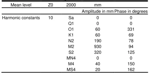
This model is forced by water level at sea boundaries and river discharges at land boundaries. The former are calculated by the equations and the harmonic components for the Faro-Olhão harbour (cf. – Fig.1-1) described in SHOM (1984) and listed in Table 2-1. Regarding the latter, only River Gilão (Fig. 1-1) was considered in the simulations described in this report, with a flow of 30 m3s-1 (winter flow estimated from rainfall).

Table 2-1 – Mean water level and harmonic constants for the Faro-Olhão harbour according to SHOM(1984).

Mean level Z0 2000 mm

Amplitude in mm Phase in degrees

Harmonic constants 10 Sa 0 0

Q1 0 0

O1 60 331

K1 60 69

N2 190 78

M2 930 94

S2 320 125

MN4 0 0

M4 40 150

MS4 20 162

2.2 Model implementation

Fig. 2-3 – EcoDynamo interface...

2.3 Model calibration and validation

Tavira-Cabanas Tavira-Clube Naval

Fuzeta-Canal

Olhão – Canal de Marim Faro-Harbour

Ancão

Olhão

Faro – main channel

Fig. 2-4 – GIS image showing the location of current meter and tide-gauge stations surveyed by the Portuguese Hydrographic Institute in 2001 (IH, 2001) and used for

model calibration (see text).

Model simulations were carried out for the same period over which current velocity and tide gauge measurements were available (January 2001 - ). The same time period was used for all simulations described in this report (see below).

2.4 Analysis of general circulation patterns and residence

times

Simulations were carried out to analyse general circulation patterns and to estimate water residence time (WRT). The former were analysed through vector plots. WRT was estimated by “filling” the lagoon with salt water and the ocean with fresh water and running the model until the lagoon water was “washed” to the sea.

Simulation results were used to calculate input, output and residual flows across Ria Formosa inlets (see Fig. 1-1) in order to get an overall picture of lagoon circulation and the relative importance of the different inlets.

2.5 Dilution of effluents from Waste Water Treatment Plants

There are several WWTPs inside the limits of the Ria Formosa Natural Park (RFNP), discharging their effluents into the lagoon waters. The geographical distribution of the WWTPs is shown in Fig. 2-5.

In order to evaluate the dispersion patterns of the effluents from WWTPs, a conservative tracer was discharged as an effluent from each WWTP (only one WWTP was considered in each simulation). The discharge occurred for the first six hours of the first simulation day. A total of 140 hours were simulated. The tracer dispersion and concentration decrease were later analysed.

Northwest Faro

East Faro

West Olhão

East Olhão Fuzeta

Pedras d’el Rei 1 Pedras d’el Rei 1

Sta Luzia Tavira

Cabanas

Northwest Faro

East Faro

West Olhão

East Olhão Fuzeta

Pedras d’el Rei 1 Pedras d’el Rei 1

Sta Luzia Tavira

Cabanas

3 Results and Discussion

3.1 Model calibration and validation

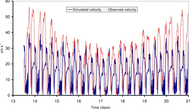
In the next figures, measured and predicted current velocities (Figs. 3-1 – 3-6) and water levels (Figs. 3-7 – 3-10) are shown for each of the monitoring locations depicted in Fig. 2-4. Regarding both current velocities and water levels, the visual fit between measurements and observations is generally good, except for current velocities at stations Tavira-Cabanas and Tavira-Clube Naval (Figs. 3-5 and 3-6).

Current speeds range from nearly zero till values in excess of 100 cm s-1. Velocity peaks occur both at the middle of the ebb and the middle of the flood. This is a normal phenomena in inlets - when current switches from flood to ebb, the water level is near its peak flood value (Militello & Hughes, 2000).

0 10 20 30 40 50 60

13 14 15 16 17 18 19 20 21

Time (days)

c

m

s

-1

Simulated velocity Observed velocity

0 10 20 30 40 50 60 70 80 90 100 110

1 2 3 4 5 6 7 8 9

Time (days)

Simulated velocity Observed velocity

c m s -1 0 10 20 30 40 50 60 70 80 90 100 110

1 2 3 4 5 6 7 8 9

Time (days)

Simulated velocity Observed velocity

c

m

s

-1

Fig. 3-2 – Predicted and measured velocities at Olhão – Canal de Marim (cf. – Fig. 2-4).

0 10 20 30 40 50 60 70

14 15 16 17 18 19 20 21

Time (days)

c

m

s

-1

Simulated velocity Observed velocity

Fig. 3-3 – Predicted and measured velocities at Faro-Harbour (cf. – Fig. 2-4).

0 10 20 30 40 50 60 70 80 90 100

2 3 4 5 6 7 8 9 10

Simulated velocity Observed velocity

c m s -1 0 10 20 30 40 50 60 70 80 90 100

2 3 4 5 6 7 8 9 10

Simulated velocity Observed velocity

c

m

s

0 10 20 30 40 50 60 70 80

13 14 15 16 17 18 19 20 21 22 23

Time (days)

c

m

s

-1

Simulated velocity Observed velocity

Fig. 3-5 – Predicted and measured velocities at Tavira-Cabanas (cf. – Fig. 2-4).

0 10 20 30 40 50 60 70 80 90 100 110

1 2 3 4 5 6 7 8

Time (days)

Simulated velocity Observed velocity

c m s -1 0 10 20 30 40 50 60 70 80 90 100 110

1 2 3 4 5 6 7 8

Time (days)

Simulated velocity Observed velocity

c

m

s

-1

Fig. 3-6 – Predicted and measured velocities at Tavira-Clube Naval (cf. – Fig. 2-4).

0 50 100 150 200 250 300 350 400

13 14 15 16 17 18 19 20 21 22

Time (days)

c

m

Observed Simulated

0 50 100 150 200 250 300 350 400

3 4 5 6 7 8 9 10

Time (days)

c

m

Observed Simulated

Fig. 3-8 – Predicted and measured water levels at Olhão (cf. – Fig. 2-4).

0 50 100 150 200 250 300 350 400

1 2 3 4 5 6 7 8 9 10

Time (days)

c

m

Simulated Observed

Fig. 3-9 – Predicted and measured water levels at Fuzeta - Canal (cf. – Fig. 2-4).

0 50 100 150 200 250 300 350 400

0 1 2 3 4 5 6 7 8 9

Time (days)

c

m

The slope of the Model II regression between measured and observed values (cf. – 2.4) was s.d. from one and the y-intercept was s.d. from zero (p > 0.05) in almost all simulations. The variance explained by the model was significant (p << 0.05) in all cases. These results imply that the model explains a significant proportion of the observed variance. However, it tends to underestimate measured velocities. This may be partially explained by the relatively low model resolution (100 m, cf. – 2.2) for such a complex flow network, with many intertidal areas and narrow channels (cf. – 2.1). Furthermore, model velocity results correspond to spatially integrated values for each cell grid, whereas measurements are performed in one point in space. Therefore, it is expectable that the former tend to be smaller than the latter.

The analysis of general ebb and flood currents in Ria Formosa (Fig. 3-11) shows that there is hardly any direct flow between its western and the eastern sides, separated by a vertical line in Fig. 3-11. Therefore, it was decided to split model domain in two – a western and an eastern domain – using a higher resolution (50 m) in the latter. This splitting procedure implies important gains in computing speed, by reducing grid size from the original 282 lines and 470 columns (cf. – 2.1) to 182 lines and 300 columns, for the western sub-domain, and 69 lines and 300 columns, for the eastern sub-domain. This also allows using a larger spatial resolution in the eastern side, where more detail is needed to simulate the narrow channels and the interface with River Gilão.

1.16 m s-1

0.96 m s-1

Ebb

Flood

1.16 m s-1

0.96 m s-1

Ebb

Flood

1.16 m s-1 1.16 m s-1

0.96 m s-1 0.96 m s-1 0.96 m s-1

Ebb

Flood

Fig. 3-11 – General circulation patterns during the flood and during the ebb. The vertical line separates the Western Ria from the Eastern Ria and the two rectangles represent the possible two sub-domains that can be considered in future simulations

0 10 20 30 40 50 60 70 80 90 100 110

1 2 3 4 5 6 7 8

Time (days)

c

m

s

-1

Simulated velocity Observed velocity

Fig. 3-12 – Predicted and measured velocities at Tavira-Clube Naval (cf. – Fig. 2-4).

0 10 20 30 40 50 60 70 80

13 14 15 16 17 18 19 20 21 22 23

Time (days)

c

m

s

-1

Simulated velocity Observed velocity

3.2 Analysis of general circulation patterns and residence

times

General circulation patterns within Ria Formosa are shown in Figs. 3-14-3-16, during the flood and during the ebb, for the Western and the Eastern Rias. Maximum current velocities are observed at the inlets. During the ebb, water remains only in the main channels. Residual flow at the Western Ria suggests the existence of eddies near the inlets and also close to Faro-Harbour (cf. – Fig. 2-4). River Gilão, located in the Eastern Ria (Figs. 3-15 and 3-16) explains the most noticeable residual flow. A 30 m3s-1 flow was used in the present simulations from rainfall-based estimates.

According to IH (2001), average ebb current velocities are higher than flood velocities for the monitoring stations depicted in Fig.2-4: Tavira-Cabanas, Tavira-Clube Naval and Olhão-Canal de Marim. The opposite is true for Fuzeta-Canal, whereas no difference was observed for the remaining two stations. These results suggest that the eastern narrow channels are ebb dominated, according to Militello & Hughes (2000).

ms-1

ms-1

Ebb

Flood

ms-1

ms-1

Ebb

Flood

ms-1

ms-1

Ebb

Flood

ms-1

ms-1

Ebb

Flood

Fig. 3-15 – General circulation patterns during the ebb and during the flood at the Eastern Ria (see text).

River Gilão

ms-1

ms-1

“Western” Ria

“Eastern” Ria

ms-1

ms-1

“Western” Ria

“Eastern” Ria

Fig. 3-16 – Residual flows at the Western and the Eastern Rias (see text).

0 50 100 150 200 250 300 350 400

0 50 100 150 200 250

Hours W a te r le v e l (c m) -150 -100 -50 0 50 100 150 C u rr e n t v e lo c it y ( c m s -1 ) Elevation (cm) Current speed

Fig. 3-17 – Measured water levels and current velocities at Fuzeta-Canal (cf. – Fig. 2-4). Flood and ebb velocities plotted as positive and negative, respectively (see text).

Table 3-1 – Predicted average ebb and flood current velocities and periods at the current meter stations depicted in Fig. 2-4 (see text).

Ebb Flood

Station Average current

velocity (cm s-1) Period (h) velocity (cm sAverage current -1) Period (h)

Ancão 17.90 7.16 24.57 5.20

Faro-Harbour 50.69 6.10 39.49 6.06 Olhão-Canal de

Marim

32.30 6.72 31.07 5.47

Fuzeta-Canal 28.49 6.25 37.92 4.94 Tavira-Clube

Naval 38.56 6.16 33.25 6.16

The integration of flows across the inlets made possible to estimate their average input-output values for a period of a month. In Fig. 3-18, a synthesis of obtained results over the whole Ria shows that the Faro-Olhão inlet is by far the most important, followed by Armona, Tavira, “new”, Cabanas and Fuzeta inlets. It is also apparent that the Faro-Olhão has a larger contribution as an inflow pathway, whereas the remaining ones contribute more as outflow pathways. The difference in input and output flows over the integration period was a 114 m3s-1input, for the Western Ria, and a 46 m3s-1output, for the Eastern Ria.

“new” inlet “new” inlet Faro-Olhão Faro-Olhão Armona Fuzeta Tavira Cabanas 226 142 1768 2033 1082 1133 141 157 149 227 246 175 “new” inlet “new” inlet “new” inlet “new” inlet Faro-Olhão Faro-Olhão Faro-Olhão Faro-Olhão Armona Fuzeta Tavira Cabanas 226 142 1768 2033 1082 1133 141 157 149 227 246 175

Fig. 3-18 – Averaged inflows and outflows (m3 s-1) through Ria Formosa inlets (see text).

3-1). The results presented in Table 3-1 suggest that flood period is larger or equals the ebb period. This may result from ebb water taking more time to reach the ocean by outflowing only thought nearby inlets, whereas during the ebb, there seems to some volume redistribution among different inlets.

Days

Days

Fig. 3-19 – Half residence time (a) and time for 90% washout (b) of Western Ria water (see text).

a

Figs. 3-19 and 3-20 show the estimated half residence and the time for the washout of 90% of lagoon water (cf. – 2.4). As expected, areas located near inlets have relatively small residence times, of less than five days, for the removal of 90% of their water, whereas inner areas, may have a half residence time of over two weeks. This is more evident in the Eastern Ria, due of its narrow inlets.

Fig. 3-20 – Half residence time (a) and time for 90% washout (b) of eastern lagoon water (see text).

a

3.3 Dilution of effluents from Waste Water Treatment Plants

Figs. 3-21 and 3-22 show the concentration decay of the tracer introduced through the Northwest Faro and Fuzeta WWTPs, and through the East and West Olhão WWTPs, respectively (cf. – 2.7). For comparison purposes, a reference concentration of 0.005 concentration units was assumed. From these figures it is apparent that the WWTP location exhibiting a faster decay, among those analysed, is the West Olhão WWTP. The semi-diurnal tidal harmonic effect over concentration, at the discharge point is more visible for this WWTP than for the remaining ones.

Figs. 3-23 and 3-24 show the evolution of the conservative tracer concentration released from the Northwest Faro WWTP and its dispersion through the lagoon channel after 2, 10 and 40 and 120 hours of simulation, respectively. During the first hours, the tracer disperses to the sea through the main channels, but as the simulation approaches the end, part of the tracer gets trapped in the inner western channels.

Main soil uses in the surroundings of the WWTPs are depicted in Fig. 3-25. For example, the Northwest Faro WWTP discharge point is located in a fishpond area, suggesting a high degree of sensitivity to effluent discharges. There are also salt marshes in this area, which enhance the ecological significance of the place. In other zones such as the West Olhão WWTP, there are shellfish growing areas, the quality of which is compromised by bacterial contamination. Furthermore, episodes of high shellfish mortalities have occurred in these areas.

Fig. 3-23 – Tracer concentration two and ten hours after the beginning of the simulation (Northwest Faro WWTP) (see text).

Fig. 3-24 – Tracer concentration 40 and 120 hours after the beginning of the simulation (Northwest Faro WWTP) (see text).

4 Conclusions

The hydrodynamic model presented in this report has been compared with real data. The visual fit of the model looks quite good for the majority of monitoring stations, both in terms of current velocities and water levels. The statistical analysis based on Model II regression between measured and simulated results shows that the model explains a significant amount of system variability. However, it tends to underestimate current velocities. This underestimation may be justified by spatial integration of model predictions (100 m) compared with the current velocity measurements, undertaken at one point in space. Since no efforts were carried out to tune the model results towards observations, it is reasonable to assume that the model appears to be reasonably validated.

The model was used to analyse general circulation patterns in Ria Formosa, showing the dominant contribution of the Faro-Olhão and Armona inlets for the lagoon-sea water exchanges and the variability in water residence time at different areas of the lagoon.

5 References

1) Pereira, A. & P. Duart, 2005. EcoDynamo Ecological Dynamics Model Application. University Fernando Pessoa.

2) Falcão, M, Fonseca, L., Serpa, D., Matias, D., Joaquim, S., Duarte, P., pereira, A., Martins, C. & M.J. Guerreiro, 2003. Synthesis report. EVK3-CT-20022-00084 (DITTY Project).

3) Instituto Hidrográfico (IH), 2001. Proj. OC4102/01, Maria Formosa, Relatório Técnico Final, Rel. TF. OC 04/2001, Monitorização Ambiental. Instituto Hidrográfico, Divisão de Oceanografia.

4) Laws, E.A., Archie, J.W., 1981. Appropriate use of regression analysis in marine biology. Marine Biology 65, 99 – 118.

5) Mesplé, F., Trousselier, M., Casellas, C. & P. Legendre, 1996. Evaluation of simple statistical criteria to qualify a simulation. Ecological Modelling 88, 9 – 18.

6) Press, W.H., Teukolsky, S.A., Vetterling W.T. & B.P. Flannery, 1995. Numerical recipes in C - The art of scientific computing. Cambridge University Press, Cambridge.

7) Militello, A. & S.A. Hughes, 2000. Circulation patterns at tidal inlets with jetties. US Army Corps of Engineers.

8) Neves, R.J.J., 1985. Étude expérimentale et modélisation mathématique des circulations transitoire et rédiduelle dans l’estuaire du Sado. Ph.D. Thesis, Université de Liège.

9) Service Hydrographique et Océanographique de la Marine (SHOM), 1984. Table des marées des grands ports du Monde. Service Hydrographique et Océanographique de la Marine, 188 pp.

10)Sokal, R.R. and F.J. Rohlf, 1995. Biometry, The principles and practise of statistics in biological research. W.H. Freeman and Company, 887 pp.

11)Vreugdenhil, C.B., 1989. Computational hydraulics, An introduction. Springer-Verlag, 183 pp.