RBRH, Porto Alegre, v. 22, e23, 2017
Scientiic/Technical Article
http://dx.doi.org/10.1590/2318-0331.011716058
Principle of maximum entropy in the estimation of suspended sediment
concentration
Princípio da entropia máxima na estimativa da concentração de sedimentos em suspensão
Patrícia Diniz Martins1 and Cristiano Poleto2
1Universidade Federal do Triângulo Mineiro, Uberaba, MG, Brazil 2Universidade Federal do Rio Grande do Sul, Porto Alegre, RS, Brazil E-mails: [email protected] (PDM), [email protected] (CP)
Received: May 13, 2016 - Revised: September 22, 2016 - Accepted: November 27, 2016
ABSTRACT
The concern with water quality has been promoting development of better monitoring and control techniques every day. As sediments transport most of water contaminants, their study is fundamental. Given the large number of variables for estimating sediment concentration and high costs of monitoring campaigns, it becomes necessary to develop more accessible methods which bring satisfactory practical results. Therefore, this work deals with application of the principle of maximum entropy, a probabilistic method to determine concentration of sediments in river channels with various concentrations and particle sizes. For this purpose, it was proposed a relationship between the theory of entropy parameters in order to reduce the computational effort. The results were satisfactory at concentrations above 10 g/L with R2 greater than 0.88. The calculated squared errors in this study were lower than those found when using the theory of entropy by Tsallis and the equation of Rouse, classic models for determining the sediment concentration proile.
The applicability of the proposed model and the ease of using the probabilistic method, since it reduces the amount of data needed to perform the estimate, makes it feasible on a global scale.
Keywords: Sedimentology; Water resources; Modeling.
RESUMO
A preocupação com a qualidade das águas vem promovendo o desenvolvimento de técnicas cada dia melhores de monitoramento e controle. Como os sedimentos transportam a maior parte dos contaminantes da água, seu estudo é fundamental. Diante do elevado número de variáveis existentes para a estimativa da concentração de sedimentos e elevados custos de campanhas de monitoramento, torna-se necessário o desenvolvimento de métodos mais acessíveis e que tragam resultados práticos satisfatórios. Para tanto, este trabalho trata da aplicação do princípio da entropia máxima, um método probabilístico, para determinar a concentração de sedimentos em calhas com diversas concentrações e granulometrias. Para isso, foi proposta uma relação entre os parâmetros do princípio da entropia máxima para determinar o índice entrópico e facilitar o cálculo. Os resultados mostraram-se satisfatórios para concentrações acima de 10 g/L com R2 superiores a 0,88. Os erros quadráticos calculados neste trabalho foram inferiores aos encontrados quando utilizada a teoria da entropia por Tsallis e pela Equação de Rouse, modelos clássicos de estimativa do peril de concentração de sedimentos. A aplicabilidade
do modelo proposto e a facilidade da utilização do método probabilístico, já que reduz a quantidade de dados necessários para realizar a estimativa, torna-o viável em escala global.
INTRODUCTION
Concern about water resources is now a reality. It is known that the amount of water is not changed on the planet, but its distribution and quality make it impossible to use. Poleto et al. (2009) state that most of water contamination is due to sediments,
especially the ine sediments that are transported to distant areas.
In urban areas this effect is greater due to large diffuse pollution. In order to identify and solve this problem, programs for monitoring the quantity and quality of sediment should be made feasible in an integrated water resources management system. However, resources are limited to serve the entire national territory. It is necessary to use more accessible techniques which bring satisfactory practical results.
The knowledge of the sediment transport rate is necessary for a number of purposes such as control and management of watersheds, river channels, sedimentation in reservoirs and
transport of pollutants. To determine this, it is necessary to ind
the average sediment concentration in a section of the channel (CUI; SINGH, 2014).
Solid discharge measurement can be done by direct and indirect methods and is divided into solid discharge measurement in suspension, responsible in most cases for about 90% of the total discharge, and by the measurement of solid drag discharge, remaining with the rest of the percentage (CARVALHO, 2008).
Suspended solid discharge is the measure of transport of suspended sediment. The sediment distribution in a river section is not uniform. According to Vanoni (1977), the forces acting on the sediment particle are a function of particle size (granulometry),
low regime (laminar or turbulent), stream velocity, bed obstacles,
water temperature, and so forth. Then, for the same composition of bottom sediments, particles drag, roll or move by salting if velocity is low, and as velocity increases, some of that sediment is
carried to a zone where the low is larger, turning into suspended
sediment. The rest remains in the deepest layer of the water body (CARVALHO, 2008; SOS, 1963; WMO, 1981).
The sediment in suspension is subject to the action of
low velocity in the horizontal direction, predominantly, and
its weight (ONGLEY, 1996; MERTEN et al., 2014). For this reason, the sediment concentration has a minimum on the surface and a maximum near the bed, for a varied granulometry. Sand particles are coarser sediments and present an increasing surface
variation for the bed. The iner ones, such as silt and clay, have
an approximately uniform distribution (SOS, 1963). For this reason, the measurement at one point does not represent the concentration of the section. It is necessary to perform sampling along the section, punctual or vertical, in a number suitable for the characterization of the section.
An important consideration to be made is that direct measurements in rivers are instantaneous measurements, because
when it comes to low measurement and sediment concentration,
when collecting water at one point, the next will not be at the same time. Unless all water from the section is collected at a given time, the measurement of sediment discharge in rivers is always by sampling.
In current operations, the average sediment concentration of the section of a channel is determined with the ratio of the representative sediment concentration to the average sediment
concentration of a vertical section line. This is a common practice in sampling the average depth to directly determine the mean vertical concentration.
However, during loods and periods of unstable low, where sediment transport is signiicant, strong currents make
sampling of the average depth unfeasible. As an alternative to this situation, models that translate the average concentration into a single sample are used.
Mathematical models are developed to describe the distribution of sediment concentration from the bed to the surface of the water in channels. These models can be used to estimate the average sediment concentration quickly using point samples in rivers. Simons and Sentürk (1992) attribute to O’Brien-Chistiansen the
irst deterministic turbulent diffusion equation for the non‑uniform
sediment distribution, derived from the continuity equation that
can be used in two‑dimensional uniform turbulent low.
A classic example of a deterministic method is the Rouse equation (ROUSE, 1937). Several combinations of this equation are derived for estimating sediment concentration.
Einstein (1950) was the irst to present a proposal for the study of sediment transport based on the probabilistic concept in the description of the movement of solid particles. The theoretical model devised by Einstein is based on the intense exchange between the particles that are in movement and those that are at rest. This model expresses the equilibrium condition between these exchanges. From this, other researchers began to use the concept of probability in their studies. According to Paiva (2007), the most relevant ones were: Brown (1950) Einstein and Barbarossa (1952), Colby and Hembree (1955), Toffaleti (1969). The work of Toffaleti (1969) is based on the Einstein method and allows the separate calculation of suspended and trailing sediments.
According to Chiu et al. (2000), models can be produced with the combination of deterministic and probabilistic concepts. The complementary feature of the two concepts strengthens the method and better describes sediment transport characteristics.
Cui and Singh (2014) compared the estimation of sediment discharge by the Tsallis entropy theory with the Prandtl von
Karman methods and the Rouse equation, and veriied that the
methods based on the entropy of both Tsallis and Shannon presented better results.
Therefore, the principle of the maximum entropy by
Tsallis is used to estimate the sediment concentration proile.
However, one disadvantage of using the entropy is in the high number of unknowns, 3 unknowns and only 2 equations, making
it an underdetermined system in which there are ininite solutions.
Due to complexity of equations, a relation was proposed between two parameters, in this way, the number of unknowns was reduced and the numerical solution became possible. The alternative formulation allows the use of 3 points of measurements in the
ield, maximum and minimum concentration, and any point
in the vertical to estimate the average sediment concentration. This facilitates estimation of sediment concentration and reduces
ield sampling time.
for concentrations above 10 g/L in all studied proiles, regardless of granulometry and low conditions.
Entropy theory
In 1824, the French physicist Carnot envisioned the
Second Law of Thermodynamics in his studies on the low of energy. By 1877, the Austrian Ludwig Boltzmann for the irst
time introduced the statistical concept of entropy, establishing a direct relationship between entropy and molecular disorder of a random thermal process, according to Resnick (2008).
Recently, Capek and Sheehan (2004) presented 21 formulations of entropy that can be divided into 5 categories according to the application: 1) devices and process impossibilities; 2) motors; 3) balance; 4) entropy; or 5) mathematical sets and spaces.
In general, it can be said that the entropy is a variable that
relects the state in which a thermodynamic system can be found.
(CHIU, 1987; CONTE, 2005; CUI; SINGH, 2014; KUMBHAKAR; GHOSHAL, 2016; SINGH, 2011; YEVJEVICH, 1972).
Conte (2005) identiies a certain physical similarity between a hydraulic and a thermal system. The author compares these two systems as if they were two reservoirs that are disconnected at
irst: one is hot and the other is cold in the thermal reservoirs
or one is full and the other is empty in the hydraulic reservoirs. After providing a communication between the two reservoirs, hot-cold or full-empty, it will take some time to establish the
equilibrium condition of these reservoirs. In the inal state, the
two thermal reservoirs will have an average temperature and the two hydraulic reservoirs will be level. In both cases, the physical concept of entropy is present, according to the Second Law of Thermodynamics, the two systems, irreversibly, will never return spontaneously to their original state, unless a certain amount of energy is expended to perform such an operation. In the hydraulic reservoir, the energy that causes the water to move is the gravitational potential. In thermodynamic systems, it was necessary to introduce the concept of an “invisible” variable that was called
entropy, to represent the low of something moving from one
reservoir to the other. In this way, Minei (1999) points out that the Second Law of Thermodynamics consists of the description of the spontaneous change of the energy distribution, from the unequal to the balanced one. According to Minei (1999), Clausius in 1950 suggested that this process of leveling applied to all forms of energy and to all events in the Universe.
In an isolated system, the entropy always grows. Since it is a probabilistic process, it is valid only for systems composed of a very large number of particles moving chaotically, according to the law of large numbers in probability theory (MINEI, 1999).
A system is characterized by its macroscopic variables, which are those quantities that can be measured in the laboratory: volume, pressure, temperature, total energy, chemical constitution. These
quantities, however, are not suficient to fully deine the state of the
system. There are a huge number of “microscopic variables” that are
dificult to determine: the position and velocity of each individual
particle, the quantum state of atoms or molecular structure, etc.
For a “macroscopic state”, there is a very large but inite number of possible “microscopic states” deined by the distribution of
particles, atoms or molecules, in space or by distribution of energy
between them. Due to the chaotic movement and the constant shocks between them, there is a certain “microscopic state” or “complexion” at each moment. As no state has preponderance over the others, there is a continual change of “microscopic states.” The number of “microscopic states” satisfying a given “macroscopic state” is called the thermodynamic probability of the state, the statistical weight of the state, or the number of complexions. Unlike mathematical probability, which always has the value of a function of its own, the value of P is always expressed by an integer, usually very large. If a spontaneous transformation occurs in an isolated system which, as a consequence, changes the “macroscopic state” of the system, this means that the new state has a greater amount of “microscopic states” or “complexions” satisfying it than the previous one. As a result, it increases the thermodynamic probability of the system and, simultaneously, the entropy of the system (MINEI, 1999, p. 13).
Thus, Capek and Sheehan (2004) state that entropy is a macroscopic quantitative measure of microscopic disorder.
The statistical concept of entropy has evolved. In 1948, Shannon proposed a theory with more solid mathematical bases, establishing a connection between entropy and typical sequences that allowed the solution of numerous problems in the areas of coding and transmission of data in the communication systems in general. Considering the example of Hancock (1961), a student
randomly lips through a book and stops, casually, in the chapter
Discrete Probability. If he already knew the subject, he will get
little or no information from the reading. If this is your irst
contact with the topic, he will be receiving a lot of information in that reading.
Thus, what differentiates the irst situation from the second
is the notion of uncertainty, that is, the greater the uncertainty about the result of a message “state”, the greater the amount of information associated with that result. If it is possible to predict the outcome of a post-message situation in advance, then certainly no information was passed by it. The measurement of post-message “state” information must be based on the probability of occurrence of this situation. Entropy, therefore, is a measure of information or degree of uncertainty about a given system (SHANNON, 1948). Shannon’s entropy can be seen as a discrete form of the classical Boltzmann-Gibbs entropy (CAPEK; SHEEHAN, 2004).
If an event occurs and a message is transmitted to communicate it, the amount of information transmitted to the
receiver is deined by Equation 1:
log p'
Information Received p
= (1)
where: p ′ = probability of the event, next to the receiver, after the arrival of the message; p = probability of the event, next to the receiver, before the arrival of the message.
Assuming only the no-noise transmission situation, that is, the received message is the same as the transmitted message, the receiver is sure that it is receiving the correct message. Thus, the probability p’ will be 1. The amount of information will depend only on the probability of the event prior to the message, so
Equation 1 can be deined by Equation 2:
log 1 log
Information Received p p
= = −
There are other deinitions that do not involve the logarithm, but the deinition of Equation 2 is simple, since it does not lead to
contradictions and has useful properties in the analysis (MINEI, 1999). According to the same author, the numerical value of the amount of information depends on the base used for the logarithms. In the transmission of information, normal is the base 2. Thus, an information unit is called a binary digit, usually called bit (SHANNON, 1948). In a situation where there are only two equally likely alternatives, a bit of information will tell which event occurred. Minei (1999) exempliies this as in the launching of a coin. There are two alternatives, heads or tails, with equal
probabilities. The result “tails” provides the speciic amount of
information according to Equation 3:
( )
log2 log2
1
2 1 bit
2
− = =
(3)
Considering a source producing 3 symbols, A, B and C, “A” occurs with probability P(A), “B” with probability P(B) and “C” with probability P(C). The amount of information associated with “A” is −log2P A( ), the one associated with “B” is −log2P B( )
and the one associated with “C” is −log2P C( ). “A” occurs in time only with the probability P(A), “B” only with P(B) and C, only with
P(C), and the average information H is deined by Equation 4:
( )log2 ( ) ( )log2 ( ) ( )log2 ( )
H P A= P A P B− P B P C− P C− (4)
The concept of entropy is already well established and used in statistics and information theory. Generalizing the result in Equation 4 for an X source and generating m independent symbols, if the jth symbol has a probability of occurrence p (X
j), the entropy can be quantiied in terms of probability according
to Equation 5:
( )
( )
j ( j)H X p X log p X= −∑ (5)
where: p X
( )
j = the probability of the system being in state X with values of {Xj, j = 1, 2, ....}.This has been shown in ideal systems, H(X) deined by
Equation 5 is equivalent to the entropy of thermodynamics. The entropy by Tsallis is a generalization of the Boltzmann-Gibbs and Shanoon entropy (CAPEK; SHEEHAN, 2004; CUI, 2011). The main advantage of Tsallis entropy is mathematical simplicity. It has been applied to numerous different physical phenomena which are considered beyond the reach of equilibrium thermodynamics. Notably, these include non-extensive long range systems, e.g., gravitational, electrostatic, such as plasmas and multiparticles, self-gravitating systems such as galaxies and globular clusters. It was applied to self-organizing behaviors and
to chaotic systems such as inancial markets, trafic, locomotion
of microorganisms, subatomic particle collisions, and tornadoes. Unfortunately, its underlying physical base was not well established,
prompting critics to label it as just a “curve it.” Its simplicity and
adaptability, however, cannot be denied (CAPEK; SHEEHAN, 2004).
According to the concept of entropy, under conditions of static equilibrium, the system tends to have the maximum entropy over current constraints (CONTE, 2005).
However, the entropy H deined by Equation 5 is the
average information content of a data sample. If the variable X is continuous, the entropy can be expressed by Equation 6:
( ) ( ) ( )ln
H X = − p X∫ p X dX (6)
where p X( ) is the probability density function so that p X dX( )
is the probability of the variable being between X and X+dX. The maximum entropy is related to the amount of information about a variable X, which is equivalent to the maximum uncertainty of X so far measured.
The principle of maximum uncertainty reveals that the maximum entropy is a function of the number of possibilities
N that this system can ind. For example, the act of playing a
6-sided die. The maximum entropy of this system is ln6, since the probability of a given face facing upwards is the same for all faces. It can be said that the entropy decreases as information about the system increases or vice versa (CONTE, 2005).
It is 0 in purely deterministic cases in which the joint probability function p X
( )
j = 1 and (Xi) = 0 for every i other than j. Maximizing the system entropy will make uniform probability distribution possible as long as it meets the constraints.According to Minei (1999), the lower the entropy, the more unequal the energy distribution. The greater the entropy, the more balanced the distribution. In this way, the maximum entropy has the equilibrium state of a system. The spontaneous tendency is in the sense of balancing unequal distributions of energy, so everything moves in the direction of a low to a high entropy.
According to the concept of entropy, it is possible, by maximum entropy, to determine the maximum uncertainty, randomness or disorder of a system. Considering a hydrological system, the principle of maximum entropy is used to model the probability distribution of the possible state of the system. The data can be collected for parameter estimation and later validation (KUMBHAKAR; GHOSHAL, 2016).
Application of entropy in hydrology and hydraulics
In general, in the traditional approach to hydraulics, the quantities involved are treated in a deterministic manner. In fact, these quantities, represented by an average value, are sample means and should be presented statistically by a mean and a variance, considering the uncertainty of any sample mean (MINEI, 1999).
The concept of entropy as used in Information Theory provides the degree of uncertainty of a particular result in a process; therefore, for the treatment of hydrological variables, one can calculate the entropy of these variables from historical and/or measured data and thus characterize the unexpected or the inherent variability of the process (CHIU, 1987; ESPILDORA; AMOROCHO, 1973; SINGH, 1989). Several works have been developed applying the theory of entropy. In the area of water resources (SINGH, 1997; HUSAIN, 1989), in the application in hydrology (WANG; ZHU, 2001; SINGH, 1998), in historical series
of precipitation and low, mainly. In the prediction of hydrological
variables (CONTE, 2005; WEIJS et al., 2010), in the evaluation of
(SINGH; CUI, 2015; CUI; SINGH, 2014; GAN et al., 2014; LIEN; TSAI, 2003; CHIU et al., 2000; LUO; SINGH, 2011; GOMEZ; PHILLIPS, 1999; SING et al., 1988; CHIU, 1988; CHAO-LIN CHIU, 1987; SINGH; KRSTANOVIC, 1987), in
the estimation of the precipitation ratio X low (SINGH, 2012; CONTE, 2005; SONUGA, 1976), in river processes (XU; ZHAO, 2013; DESHPANDE; KUMAR, 2013), among other applications.
The velocity distribution equation derived from the principle of maximum entropy has advantages over the universal equation of velocity distribution of Prandtl-von Karman. The maximum entropy applied to the velocity distribution and sediment transport
relects the effect of particle size of suspended sediment, coarse
material and sediment concentration. They can be used as variables
to characterize and compare various lows (SINGH; CUI, 2015; CHAO-LIN CHIU, 1987).
Chiu et al. (2005) and Minei (1999) established river low estimation methods using the probabilistic model based on the Shannon entropy with the velocity measurement at only one point of a vertical of the river or some points of that river vertical. This greatly reduces the time and cost of sampling. In addition, it
makes possible the measuring during loods when the water level
undergoes large variations in a short time. This technique can be applied when using radars on the surface of water and even
ADCPs (Acoustic Doppler Current Proiler), especially during loods. The surface velocity is measured and then it is possible to ind the entropy parameters. The channel section is calculated by calculating the discharge or total low (MORIASI et al., 2007). The discharge data obtained by such methods can also be used to understand the ratios of the discharge phases occurring during
unstable high low periods, which have the forms different from those presented by the conventional classiication curves obtained with constant low periods (CHIU et al., 2005). Such advances
should add scientiic knowledge to hydrology and may also contribute greatly to engineering projects for lood control. Once the channel section is known, the discharge or total low is calculated
(CHIU et al., 2005; MORAMARCO et al., 2013). The discharge data obtained by such methods can also be used to understand the ratios of the discharge phases occurring during unstable
high low periods, which have the forms different from those presented by the conventional classiication curves obtained with constant low periods (CHIU et al., 2005). Such advances should
add scientiic knowledge to hydrology and may also contribute greatly to engineering projects for lood control.
MATERIAL AND METHODS
To determine the sediment concentration in different low
regimes and grain sizes, two data series were collected by Coleman (1981) and Einstein and Chien (1955). These two data series were
used because of their signiicance in sediment transport studies
and because they present the greatest detail of the sediment
concentration proile. These two aspects are important for the
validation of the proposed method.
For this, the conditions of accomplishment of each one
of the works under different conditions of low and granulometry
will be detailed.
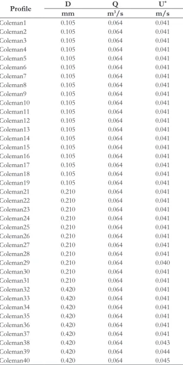
The Coleman (1981) experiment was performed on a rectangular channel 0.356 m wide and 15 m long with an adjustable
slope to maintain the low. The particle size (D), discharge (Q) and velocity (U*) of each proile are shown in Table 1.
On the other hand, the Einstein and Chien (1955) experiment was performed on a 0.31 m wide, 0.36 m deep, and 12.19 m long channel. The slope was adjusted through a connector ranging from 0.0185 to 0.025, and the discharge ranged from 0.074 to 0.085 m3/s.
The water depth (H), the mean velocity (U*) and the diameter at which 50% of the material is retained (D50) can be seen in Table 2.
Three different types of sand were used in their experiments of Einstein and Chien (1955), which were evaluated as coarse,
with D50 of 1.3 mm, medium with D50 of 0.94 mm and ine
with D50 of 0.274 mm.
Table 1. Conditions of the Coleman (1981) experiment.
Proile mmD mQ3/s m/sU*
Coleman1 0.105 0.064 0.041
Coleman2 0.105 0.064 0.041
Coleman3 0.105 0.064 0.041
Coleman4 0.105 0.064 0.041
Coleman5 0.105 0.064 0.041
Coleman6 0.105 0.064 0.041
Coleman7 0.105 0.064 0.041
Coleman8 0.105 0.064 0.041
Coleman9 0.105 0.064 0.041
Coleman10 0.105 0.064 0.041
Coleman11 0.105 0.064 0.041
Coleman12 0.105 0.064 0.041
Coleman13 0.105 0.064 0.041
Coleman14 0.105 0.064 0.041
Coleman15 0.105 0.064 0.041
Coleman16 0.105 0.064 0.041
Coleman17 0.105 0.064 0.041
Coleman18 0.105 0.064 0.041
Coleman19 0.105 0.064 0.041
Coleman21 0.210 0.064 0.041
Coleman22 0.210 0.064 0.041
Coleman23 0.210 0.064 0.041
Coleman24 0.210 0.064 0.041
Coleman25 0.210 0.064 0.041
Coleman26 0.210 0.064 0.041
Coleman27 0.210 0.064 0.041
Coleman28 0.210 0.064 0.041
Coleman29 0.210 0.064 0.040
Coleman30 0.210 0.064 0.041
Coleman31 0.210 0.064 0.041
Coleman32 0.420 0.064 0.041
Coleman33 0.420 0.064 0.041
Coleman34 0.420 0.064 0.041
Coleman35 0.420 0.064 0.041
Coleman36 0.420 0.064 0.041
Coleman37 0.420 0.064 0.041
Coleman38 0.420 0.064 0.043
Coleman39 0.420 0.064 0.044
Coleman40 0.420 0.064 0.045
The low conditions and granulometry of each of the proiles
(S) of Einstein and Chien (1955) can be visualized in Table 2.
Method for the estimation of sediment concentration
The estimation of the sediment concentration using
the Tsallis entropy implies in (1) deinition of Tsallis entropy, (2) speciication of restrictions, (3) maximization of entropy,
(4) determination of Lagrange multipliers, (5) determination of the probability density function and maximum entropy, (6) hypothesis of cumulative probability distribution, and (7) sediment concentration distribution. These steps were detailed by (CUI; SINGH, 2014) and are described below. After these steps, changes in sediment concentration distribution were performed to reduce the number of parameters and to facilitate calculations (8).
Deinition of the Tsallis entropy
Given that the concentration of sediments “c” is a random variable with function of density and probability, f(c), then the Tsallis entropy (TSALLIS, 1988) of “c”, H(c), can be expressed by Equation 7:
( ) ( ) ( )
{
( )}
Cm m Cm m 1
Ch Ch
1 1
H c 1 f c dc f c 1 f c dc
m 1 m 1
−
= − = − −
− ∫ − ∫ (7)
where c, ch ≤ c ≤ cm, is the value of the random variable c, cm is the maximum value of “c” or bed concentration, ch is the concentration on the water surface, the symbol m represents the entropy index, and H represents the entropy of f(c) or “c” (CHIU; JIN, 1997).
When m = 1, the entropy by Tsallis is equal to that of Boltzmann-Gibbs and Shanoon (CAPEK; SHEEHAN, 2004; CUI, 2011). The entropic index, non-extensivity parameter m, is considered a measure of the fractal nature of the path of a system
in phase space. It is able to show the rapid and radical changes in behavior and phase (CAPEK; SHEEHAN, 2004).
Speciication of restrictions
The f(c) is a Probability Density Function and must satisfy Equation 8: ( ) m h c c
f c dc 1 ∫ = (8)
One of the simplest constraints is the mean or equilibrium sediment concentration by volume, called cD. The mean value may be known or obtained from observations, and can be expressed by Equation 9:
( ) [ ] m h c D c
cf c dc E c= =c
∫ (9)
Entropy maximization
The entropy H of c, given by Equation 7 can be maximized, according to Jaynes (1957), using the Lagrange multiplier method. For this purpose, the Lagrange function L can be expressed by Equation 10:
( )
{
( )}
( ) ( )
m m m
h h h
c c c
m 1
0 1 D
c c c
f c
L 1 f c dc f c dc 1 cf c dc c
m 1 λ λ
−
= − − − − − − −
∫ ∫ ∫ (10)
where λ0 and λ1 are the Lagrange multipliers. Differentiating Equation 10 with respect to f, highlighting f as a variable and “c” as a parameter, and equating the derivative to zero, it is obtained:
( )
m 1 0 1
L 1
0 1 mf c 0
f m 1 λ λ
−
∂ = → − − − =
∂ − (11)
Equation 11 leads to Equation 12
( )
1 m 1 0 1
m 1 1
f c c m m 1 λ λ
− − = − − − (12)
which represents the less biased density and probability function of sediment concentration “c” based on Jaynes (1957).
Determination of Lagrange multipliers
Equation 12 has unknown λ0 and λ1 that can be determined
using Equations 8 and 9. The Lagrange multiplier λ1 is associated
with the mean concentration and λ0 with the total probability.
These multipliers have opposite signals, with λ1 positive and λ0
negative. The substitution of Equation 12 in Equation 8 leads to:
m h 1 c m 1 0 1 c
m 1 1
c dc 1
m m 1 λ λ − − − − = −
∫ (13)
The integration of Equation 13 will be:
m m m
m 1 m 1 m 1
0 1 m 0 1 h
1
1 m 1 1 1
c c 1
m m 1 λ λ m 1 λ λ
λ − − −
− − − − − − − = − − (14)
Table 2. Conditions of the Einstein and Chien (1955) experiment.
Proile H U* D50
mm m/s mm
RunS1 138 0.115 1.3
RunS2 120 0.129 1.3
RunS3 120 0.133 1.3
RunS4 115 0.144 1.3
RunS5 109 0.144 1.3
RunS6 142 0.118 0.94
RunS7 142 0.118 0.94
RunS8 139 0.115 0.94
RunS9 135 0.118 0.94
RunS10 128 0.125 0.94
RunS11 133 0.0767 0.274
RunS12 132 0.0767 0.274
RunS13 134 0.0767 0.274
RunS14 124 0.0767 0.274
RunS15 124 0.0767 0.274
RunS16 119 0.0767 0.274
Likewise, the substitution of Equation 12 in Equation 9 will be: m h 1 c m 1
0 1 D
c
m 1 1
c c dc c
m m 1 λ λ − − − − = −
∫ (15)
Equation 15 can be integrated by parts such as:
m m
m 1 m 1
1 D m 0 1 m
m m 1
h 0 1 h
1
2m 1 2m 1
m 1 m 1
0 1 m 0 1 h
m 1
c c c m 1 m 1
1 m 1 1 c c
m 1 2m 1
1 1
c c m 1 m 1
λ λ λ
λ λ λ
λ λ λ λ
− − − − − − − − − = − − − − − − − − − + − − − − − − − − − (16)
Equations 14 and 16 can be solved numerically for λ0 and
λ1 for speciied values of c, cm, ch, and m.
Determination of the Cumulative Distribution Function (CDF) and maximum entropy
Integrating Equation 12 from ch to c yields the Cumulative Distribution Function of c, F(c), according to:
( )
m m m
m 1 m 1 m 1
0 1 h 0 1
1
m 1 1 1 1
F c c c
m λ m 1 λ λ m 1 λ λ
− − −
−
= − − −− − −− −
(17a)
If the low of sediments on the water surface is insigniicant,
that is, ch = 0, then Equation 17a becomes:
( )
m m m
m 1 m 1 m 1
0 0 1
1
m 1 1 1 1
F c c
m λ m 1 λ m 1 λ λ
− − − − = − − −− − − − (17b)
Now, the maximum entropy of c is obtained by inserting Equation 17b into Equation 7:
( ) ( )
m m 1
m h
1
2m 1 2m 1
m 1 m 1
0 1 m 0 1 h
m 1 1 c c
m 2m 1 1
H c m 1
1 1
c c m 1 m 1
λ
λ λ λ λ
− − − − − − − + + + − = − − − − − − − − − (18)
Equation 18 is expressed in terms of λ0 and λ1, Lagrange multipliers, by the lower limit of concentration, ch, and upper limit of concentration cm.
Cumulative Distribution Function (CDF)
The cumulative distribution function of “c”, F(c), in terms
of low depth can be written as:
( ) 0
0 0
h y y
F c 1
h− h
= = − (19)
Equating Equation 19 with Equation 17a, it becomes:
( )
m m m
m 1 m 1 m 1
0 1 h 0 1
1 0
m 1 1 1 1 y
F c c c 1
m − λ m 1 λ λ − m 1 λ λ − h
− = − − − − − − − − = − (20)
Distribution of sediment concentration
For simplicity, considering * 1 1
m 1
λ = − −λ , then Equation 20 can be written as:
( )
m 1 m m m 1 *
1 * 1 h
1 1 0
1 m m 1 y m 1
c 1 c
m 1 m h m
λ λ λ λ
λ λ − − − − = − − − − + − − (21)
If ch = 0, Equation 21 reduces to:
m 1 m m m 1 *
1 *
1 1 0
1 m m 1 y m 1
c 1
m 1 m h m
λ λ λ
λ λ − − − − = − − − − + (22)
Equation 22 represents the deined sediment concentration distribution in terms of low depth.
Reparametrization
The distribution of sediment concentration can be simpliied using a dimensionless entropy parameter deined as:
1 m
1 m * 1
c 1 m
c m 1
λ
µ λ= −λ −λ − (23)
Dividing Equation 22 by cm, we obtain:
m 1 m m m 1 *
1 *
m 1 m 1 m 0
c 1 m m 1 1 y m 1
c λλc λc m 1 λ m h m λ
− − − − = − − − − + (24)
Since * 1 m
1 1
c λ
λ = −µ, μ from Equation 23, Equation 24 can
be reformulated as:
m 1
m m
m 1
m m 0
c 1 m y
1 1 1
c µ m 1 cµ h
− − = − − − − + (25)
If ch = 0 at y = h0, Equation 25 reduces to:
m 1
m m
m 1 m
1 m
0 1 1 1 m 1 c
µ µ − − = − − − − (26)
Equation 26 suggests:
( ) m m m 1 m 1 m m 1 1 m 1 c
µ µ
−
−
= − −
−
(27)
( ) ( )
m 1
m m m
m 1 m 1
m 0
c 1 1 1 1 1 1 1 y
c µ µ µ h
− − − = − − − + − − − − (28)
Equation 28 expresses the sediment concentration distribution as a function of the vertical distance y.
Reduction of parameters
In order to estimate the sediment concentration distribution in a given section, it was used the probabilistic model of Cui and Singh (2014), which can be visualized in Figure 1, expressed by Equation 29: ( ) m 1 m m a m 1 *
1 * 1 h
1 1 0
1 m m 1 y m 1
c 1 c
m 1 m h m
λ λ λ λ
λ λ − − − − = + − − − + + + (29)
Since * 1
1 m 1
λ = −λ
− where:
c = concentration of sediments at a vertical distance y, dimensionless; cm = maximum value of C or concentration in the bed, dimensionless; ch = concentration on the water surface, dimensionless; m = entropy
parameter, dimensionless; λ1 = Lagrange multiplier, dimensionless; h0 = depth of low, in meters; a = parameter related to the characteristics of sediment particles.
Equation 29 differs from Equation 22 by the introduction of parameter “a” which is related to particle characteristics such as size, roughness, among others (CUI; SINGH, 2014).
Equation 29 can be rewritten to any point (Equation 30) and to the one with the highest sediment concentration at the deepest point of the river (Equation 31).
( ) m 1 m m a m 1 *
1 * 1 h
1 1 0
1 m m 1 y m 1
c 1 c
m 1 m h m
λ λ λ λ
λ λ − − − − = + − − − + + + (30) ( ) ( ) m 1 m m m 1 a *
m 1 * 1 h
1 1
1 m m 1 m 1 c 1 c
m 1 m m
λ λ λ λ
λ λ − − − − = + −− + + (31)
Reorganizing Equation 29 suggested by Cui and Singh (2014), we have:
( ) m 1 m m a m 1 *
1 * 1 h
m 1 m 1 h 0
1 1 1 m m 1 1 y m 1 c
c c λλc λc m 1 λ m h m λ λ
− − − − = − − − − + − − (32)
Inverting Equation 31 deduced in this work, it becomes:
( ) ( ) 1 m m m m 1 a 1
1 * 1 h
m 1
1 m 1 m 1 1 c c 1 m m
λ λ λ λ
λ − − − − = + − + − (33)
Equating Equations 32 and 33:
( ) ( ) ( ) ( ) ( ) m 1 m m a m 1 *
1 * 1 h
1 1 0
1 m
m m
m 1
a
1
1 * 1 h
1
1 1 m m 1 1 y m 1 c
c Cm Cm m 1 m h m
m 1 m 1 m 1
1 c
m 1 m m m
λ λ λ λ
λ λ
λ λ λ λ
λ − − − − − − − − − + − − = − − − − + − − − − − (34)
Simplifying the equality expressed in Equation 34,
considering ( ) ,
m
a
m 1
1m 1 y m 1 * 1 h
T1 1 c
m D m
λ − − λ λ −
= − − + +
and
( ) ( )
m m 1
a
1m 1 m 1 * 1 h
T 2 1 c
m m
λ − − λ λ −
=
− + +
, we have:
( )
( ) ln( )
2 1 1
1 m 1
ln T1T 2 0
1 CCm m
λ λ
+ −
+ =
+
(35)
Therefore, we obtain a system with three unknowns: λ1 ,
,
a e m and two equations. The variables ch, c and cm, as well as y
and h0 must be obtained in the ield data. In this work the relation of m=expF c( )λ1.
Equation 35 is the basis of the developed method. Unlike previous work, the minimum concentration is not considered as 0.
In the simulation, besides the relation m=expF c( )λ1 of m,
it was adopted the function a a'= ((y ho *22/ ) ) For the parameter “a”,
where a’ is a parameter to be measured, y is the depth of the point and ho is the maximum depth. As well as “m”, a’ is determined by the solution of the system detailed in the item “Reduction of parameters”, presented in Equation 35, taking into consideration T1 and T2.
Validation
In order to evaluate eficiency of the model, the following statistical coeficients were applied: Nash‑Sutcliffe eficiency (NSE); coeficient of determination (R2); Deviation between observed and simulated lows (D%); Pbias; ratio of the root
mean square error to the standard deviation of measured data (RSR); e root-mean-square error (RMSE). Subsequently, their formulations are presented, where cobs and ccalc refer to the observed and calculated concentrations, respectively, in g/L.
According to Molnar (2011), the value of the Nash-Sutcliffe
coeficient indicates the adjustment of the simulated data to those observed in the 1: 1 line, which can vary from ‑∞ to 1. Molnar
Figure 1. Uniform low of sediments. Where c (y) = concentration
of sediments at a vertical distance y, dimensionless; cm = maximum value of C or concentration in the bed, dimensionless; ch = concentration on the water surface, dimensionless; h0 = depth
(2011) presented the following classiication for this coeficient, using daily simulation step: NSE> 0.8 the model is considered excellent; 0.8 <NSE <0.6 the model is considered very good; 0.4 <NSE <0.6 the model is considered good, between 0.4 and
0.2, satisfactory and <0.2 insuficient. According to Moriasi et al. (2007), NSE values above 0.5 qualify the model for simulation.
(
)
(
)
2 N obsi calci i 1 2 N obsi obs i 1 c c NSE 1 c c = = − = − − ∑∑ (36)
The R2 value, according to Willmott et al. (1985), is an
indicator of the correlation between observed and simulated values, with amplitude of variation between 0 and 1, where the
value 1 indicates a perfect it. This coeficient is considered one
of the most sensitive statistics to extreme values. R2 values above 0.5 are considered as acceptable (Moriasi et al., 2007).
(
) (
)
(
)
.(
)
.N
obsi obs calci calc i 1
2
0 5 0 5
2 2
N N
obsi obs calci calc
i 1 i 1
c c * c c
R
c c * c c
= == − − = − − ∑
∑ ∑ (37)
The value of D means the average trend of the estimates produced by the model and, when positive, expresses a tendency of overestimation and when negative, of underestimation. Liew et al. (2003) cited by Viola et al., (2012) present the following ranges and respective interpretations of D: <10%, very good; between 10% and 15%, good; between 15% and 25%, satisfactory and> 25%, the model produces inadequate estimates regarding the trend.
( )
N calci obsi i 1 obsi c c *100 c D % N = −
=∑ (38)
Pbias also measures deviation of data. When positive, the model tends to overestimate the data and when negative, to underestimate the simulated data in relation to the measured ones. An ideal model would have a value of 0.
( ) i 1N ( obsi( )calci) N
obsi i 1
c c *100
Pbias % c = = − =∑
∑ (39)
RSR is the relation between the root mean square error to the standard deviation of measured data:
( ) ( ) 2 N calci obsi i 1 2 N
obs obsi médio i 1
c c
RMSE RSR
STDEV = c c
=
−
= =
− ∑
∑ (40)
The root-mean-square error allows to quantify the magnitude of the deviations of the simulated values in relation to the observed ones. The closer to 0, the better the data adjustment. It is expressed by:
( )2
N
calci obsi i 1c c RMSE
N
= −
= ∑ (41)
Moriasi et al. (2007) reported intervals of values and performance evaluations for the recommended statistics and
established guidelines for evaluation of low simulation models,
sediment transport and nutrients. Based on this analysis, they
recommended three quantitative statistics: Nash‑Sutcliffe eficiency
(NSE), percent bias (Pbias) and ratio of the root mean square error to the standard deviation of measured data (RSR), besides the graphic techniques, to be used in the evaluation of models. In general, model simulation can be judged to be satisfactory if NSE> 0.50 and RSR <0.70, and if PBIA <= 55% for sediments.
RESULTS AND DISCUSSION
Using the relation of m=expF c( )λ1, it was possible to
reduce the solution of sediment concentration proile estimation
to 2 unknowns.
It is possible to note in Figure 2 the estimate made with the data of Coleman (1981). The proiles from 2 to 20 correspond to group 1, from 22 to 31 group 2 and 33 to 40 group 3. The data from group 1 have a granulometry of 0.105 mm, group 2 of 0.210 mm and group 3 of 0.420 mm. All Coleman data were simulated with
a constant low of 0.064 m3/s. Concentrations were minimal in the irst experiments of each group increasing until the last. Proiles 1, 21 and 32 had the concentration 0 and are not mentioned. Proiles 20, 31 and 40 had the highest concentrations.
It can be observed (Figure 2) that the model is better suited
to proiles with high concentrations. Proiles 2, 3, 22 and 23 and all proiles of Group 3 show differences between the measured
and estimated values at the surface.
It can be seen from the D% value that the model
overestimated the concentrations below 5 g/L of the proiles 2 to 6
of Group 1 and 22 to 27 of Group 2 as can be proved by the D% value (see Table 3). It also overestimated the concentrations below 10 g/L with a grain size of 0.420 mm from the Group’s
33‑40 proiles. Although proiles 2, 22, 33, 34 and 35 showed unsatisfactory results for NSE, all other proiles presented
satisfactory results for R2.
Taking into account that the Pbias limit for sediments is 55%, the measured data had values smaller than those observed
only in proiles 2, 33, 34, 35 and 36. Therefore, by Pbias, there was no overestimation of the proiles 3.4, 5.6, 22, 23, 24.25, 26, 27.37, 38, 39 and 40 as veriied by D%. The limit value of D% is 25%
(LIEW et al., 2003 cited by VIOLA et al., 2012), more restrictive than that of 55% for Pbias (MORIASI et al., 2007), since it is a reference
for watershed modeling, however Pbias is speciic for sediments.
Analyzing the data according to R2 and NSE, for Group 1,
values above 0.92 and 0.84 for R2 and NSE, respectively, were obtained, except for proile 6. For Group 2, values higher than 0.89 and 0.76
were obtained for R2 and NSE, respectively, with the exception of proile 22. For Group 3, values above 0.88 and 0.72 for R2 and NSE, respectively, were obtained, except for proiles 33, 34 and 35. With the exception of proiles 2, 6, 22, 33, 34 and 35, which
present concentrations below 10 g/L, all other results presented high values, above 0.72 for NSE and above 0.88 for R2. This shows the eficiency of the proposed method.
The proiles are suitable for RSR, with values below 0.7, except proiles 2, 6, 22, 33, 34 and 35, which have concentrations
below 10 g/L.
As for RSME, it was found the highest value of 12.87.
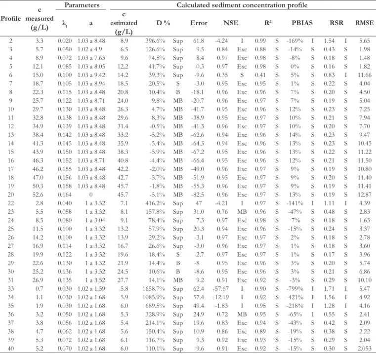
Table 3. Summary of the results of this work using data from Coleman (1981).
Proile measured c (g/L)
Parameters Calculated sediment concentration proile
λ1 a
c estimated
(g/L)
D % Error NSE R2 PBIAS RSR RMSE
2 3.3 0.020 1.03 a 8.48 8.9 396.6% Sup 61.8 -4.24 I 0.99 S -169% I 1.54 I 5.65 3 5.7 0.050 1.02 a 4.9 6.5 126.6% Sup 9.5 0.84 Exc 0.88 S -14% S 0.43 S 1.98 4 8.9 0.072 1.03 a 7.63 9.6 74.5% Sup 8.4 0.97 Exc 0.98 S -8% S 0.18 S 1.48 5 12.1 0.085 1.03 a 8.05 12.2 41.7% Sup 0.3 0.97 Exc 0.98 S 0% S 0.16 S 1.82 6 15.0 0.100 1.03 a 9.42 14.2 39.3% Sup -9.6 0.35 S 0.41 S 5% S 0.83 I 11.66 7 18.7 0.105 1.03 a 8.94 18.5 20.5% S -3.0 0.95 Exc 0.95 S 1% S 0.22 S 4.04 8 22.3 0.115 1.03 a 8.48 20.8 10.4% B -18.1 0.96 Exc 0.96 S 7% S 0.20 S 4.50 9 25.7 0.122 1.03 a 8.71 24.0 9.8% MB -20.7 0.96 Exc 0.97 S 7% S 0.19 S 5.04 10 29.7 0.130 1.03 a 8.48 26.3 4.7% MB -41.7 0.95 Exc 0.96 S 12% S 0.23 S 7.25 11 32.8 0.138 1.03 a 8.48 29.6 8.3% MB -38.9 0.95 Exc 0.97 S 10% S 0.21 S 7.94 12 34.9 0.139 1.03 a 8.48 31.4 -0.5% MB -41.3 0.96 Exc 0.97 S 10% S 0.20 S 7.70 13 38.4 0.142 1.03 a 8.48 33.2 -5.2% MB -62.6 0.94 Exc 0.96 S 14% S 0.23 S 9.47 14 41.3 0.145 1.03 a 8.48 35.9 -5.4% MB -64.3 0.94 Exc 0.96 S 13% S 0.23 S 10.45 15 43.9 0.150 1.03 a 8.48 38.3 -5.9% MB -67.2 0.95 Exc 0.96 S 13% S 0.22 S 11.22 16 46.3 0.152 1.03 a 8.71 40.8 -4.4% MB -66.4 0.95 Exc 0.96 S 12% S 0.21 S 11.50 17 46.2 0.155 1.03 a 8.48 42.2 -2.0% MB -49.0 0.96 Exc 0.97 S 9% S 0.19 S 10.80 18 47.0 0.156 1.03 a 8.48 42.7 -5.7% MB -51.9 0.95 Exc 0.97 S 9% S 0.20 S 11.40 19 50.3 0.158 1.03 a 8.48 45.7 -1.8% MB -55.3 0.96 Exc 0.97 S 9% S 0.19 S 11.41 20 52.6 0.164 0 45.7 -5.1% MB -82.5 0.96 Exc 0.97 S 13% S 0.19 S 12.87 22 2.8 0.040 1 a 3.32 7.1 416.2% Sup 47 -4.21 I 0.97 S -141% I 1.11 I 4.39 23 5.5 0.058 1 a 3.32 8.1 157.8% Sup 31.0 0.76 MB 0.96 S -47% S 0.48 S 2.83 24 8.5 0.080 1 a 3.04 9.1 78.4% Sup 7.3 0.97 Exc 0.98 S -7% S 0.18 S 1.63 25 11.5 0.100 1 a 3.32 13.2 57.9% Sup 20.3 0.94 Exc 0.96 S -15% S 0.24 S 3.37 26 14.2 0.100 1 a 3.32 13.9 29.2% Sup -3.1 0.97 Exc 0.97 S 2% S 0.18 S 2.78 27 16.9 0.114 1 a 3.32 16.7 26.6% Sup -3.0 0.96 Exc 0.97 S 1% S 0.18 S 3.60 28 19.9 0.122 1 a 3.32 19.6 18.4% S -2.7 0.97 Exc 0.97 S 1% S 0.17 S 3.96 29 22.6 0.130 1 a 3.32 21.9 14.4% B -8 0.95 Exc 0.96 S 3% S 0.20 S 5.74 30 25.2 0.136 1 a 3.32 24.5 10.6% B -8.6 0.95 Exc 0.96 S 3% S 0.21 S 6.86 31 26.9 0.135 1 a 3.52 27.7 14.1% MB 9.2 0.91 Exc 0.92 S -3% S 0.29 S 10.10 33 0.7 0.030 1.02 a 1.59 5.8 1658.7% Sup 62.4 -57.67 I 0.90 S -799% I 1.71 I 5.47 34 1.1 0.030 1.02 a 1.68 5.9 1085.9% Sup 57.4 -12.19 I 0.92 S -421% I 1.56 I 4.92 35 1.9 0.030 1.02 a 1.68 6.0 689.5% Sup 49.4 -1.83 I 0.95 S -218% I 1.28 I 4.16 36 3.2 0.050 1.02 a 1.68 5.3 328.9% Sup 24.9 0.72 MB 0.95 S -65% I 0.55 S 2.41 37 3.8 0.056 1.02 a 1.68 5.4 214.1% Sup 19.6 0.83 Exc 0.94 S -43% S 0.42 S 2.09 38 4.7 0.062 1.02 a 1.68 5.6 150.4% Sup 10.9 0.86 Exc 0.89 S -19% S 0.38 S 2.22 39 5.3 0.072 1.02 a 1.68 6.1 116.7% Sup 9.3 0.92 Exc 0.93 S -15% S 0.29 S 2.04 40 5.2 0.070 1.02 a 1.68 6.0 110.1% Sup 9.6 0.91 Exc 0.92 S -15% S 0.30 S 2.053 Where Exc = Excellent; MB = Very Good; B = Good; S = Satisfactory; Sub = Underestimate; Sup = Overestimate; I = Unsatisfactory. c = concentration of sediments
at a vertical distance y; λ1 = Lagrange multiplier, dimensionless; a = parameter related to the characteristics of sediment particles. Nash‑Sutcliffe eficiency (NSE); coeficient of determination (R2); Deviation between observed and simulated lows (D%); Pbias; ratio of the root mean square error to the standard deviation of
measured data (RSR); e root-mean-square error (RMSE).
all proiles except for proiles 2, 22, 33, 34 and 35, both with low concentrations. Proile 6 was anomalous and did not it as well.
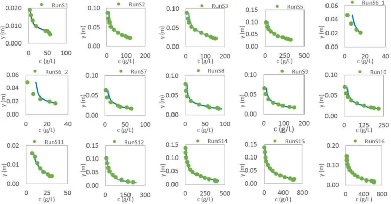
The simulation performed with Einstein and Chien (1955) is shown in Figure 3 and Table 4. Each RunS is a sediment
concentration proile with different velocities and granulometries,
detailed in Table 2.
The calibration of the model was performed based on the
coeficients of R2 and NSE. In order to identify the best results,
the parameters which brought the highest values of NSE and R2 were adopted, respectively, to the concentration proile.
The model of the present study did not overestimate or underestimate the sediment concentration of the data of Einstein and Chien (1955) according to D% and Pbias%, contrary to the data obtained by Coleman (1981).
The RSR values were satisfactory for all proiles.
In Table 4 the measured concentrations X estimated concentrations can be visualized. There are acceptable results for NSE and R2 for all proiles with NSE higher than 0.73 and R2
higher than 0.81. The cumulative distribution function (CDF) was
not well estimated only in the Run6.2 proile. This may be due to the fact that practically the whole proile is in low concentrations.
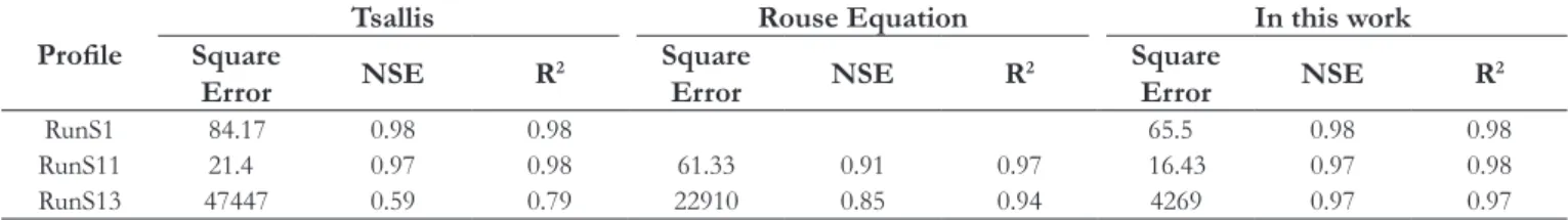
The comparison of the simulation with the results of Cui (2011) can be visualized in Figure 4 and Table 5. One can observe the adherence of the calculated and measured data.
The square error of RunS1, RunS11 and RunS13 proiles
using the Tsallis entropy theory and the Rouse Equation, as can be seen in Table 5.
Cui and Singh (2014) compared the estimation of sediment discharge by the entropy theory by Tsallis and Shannon with the same data from Coleman (1981) and Einstein and Chien (1955).
The authors observed that, although there were no signiicant
differences between the results, the Tsallis entropy theory presents more accurate results. In order to improve the results, the authors used correction factors. In the same work, they compared the results with the Prandtl von Karman methods, Rouse equation
Figure 3. Sediment concentration proiles measured by Einstein and Chien (1955) were identiied by points and calculated in this work were identiied by the continuous lines. Where y (m) is the depth of the lluxo given in meters and c (g/L) the sediment concentration
given in g/L.
Table 4. Summary of the results of this work using data from Einstein and Chien (1955).
Proile measured c (g/L)
Parameters Sediment concentration proile calculated
λ1 a
c estimated
(g/L)
D % Error NSE R2 PBIAS RSR RMSE
RunS1 34.83 0.29 1.22 a 2.93 30.49 6.4% MB -2.92 1.00 Exc 0.983 S 2% S 0.027 S 0.60 RunS2 59.92778 0.32 1.36 a 3.6 56.27 19.6% S 19.65 1.00 Exc 0.988 S -3% S 0.034 S 1.40 RunS3 77.91111 0.19 1.3 a 2.93 71.86 13.7% B 12.39 1.00 Exc 0.976 S -1% S 0.021 S 1.11 RunS4 106.9867 0.09 1.35 a 2.93 95.77 0.6% MB -13.91 1.00 Exc 0.965 S 2% S 0.016 S 1.18 RunS5 172.2778 0.03 1.03 a 1.59 162.02 12.8% B 55.53 1.00 Exc 0.998 S -3% S 0.022 S 2.36 RunS6_1 11.00333 12 1.48 a 2.37 10.43 15.4% S 6.54 0.95 MB 0.999 S -8% S 0.285 S 1.28 RunS6_2 17.9625 0.2 0.91 a 0.66 16.89 15.3% S 11.23 0.98 Exc 0.941 S 4% S 0.170 S 1.50 RunS7 34.49 0.47 1.33 a 2.86 30.17 22.6% S 2.38 1.00 Exc 0.993 S 0% S 0.028 S 0.58 RunS8 42.4775 0.45 1.22 a 2.93 37.46 23.8% S -3.53 1.00 Exc 0.981 S 2% S 0.020 S 0.63 RunS9 75.22143 0.11 1.17 a 1.88 67.53 15.4% S 10.23 1.00 Exc 0.996 S -1% S 0.022 S 1.13 RunS10 106.4688 0.09 1.2 a 2.13 98.89 18.7% S 32.60 1.00 Exc 0.988 S -3% S 0.025 S 1.90 RunS11 21.09429 13 1.27 a 2.6 21.25 -1.1% MB 2.29 1.00 Exc 0.977 S 1% S 0.061 S 0.53 RunS12 85.95125 1.09 1.17 a 3.91 81.22 21.6% S 35.62 1.00 Exc 0.985 S -4% S 0.029 S 1.99 RunS13 151.4222 0.54 1.19 a 5.55 133.74 7.2% MB -29.96 1.00 Exc 0.973 S 3% S 0.009 S 1.17 RunS14 157.72 0.59 1.19 a 6.27 141.84 22.9% S -52.48 1.00 Exc 0.969 S 43% S 0.015 S 2.01 RunS15 269.6642 0.352 1.2 a 6.39 243.83 23.8% S -72.02 1.00 Exc 0.947 S 16% S 0.011 S 2.35 RunS16 286.1833 0.45 1.18 a 5.44 267.27 18.3% S 23.86 1.00 Exc 0.962 S 26% S 0.006 S 1.35 Where Exc = Excellent; MB = Very Good; B = Good; S = Satisfactory; Sub = Underestimate; Sup = Overestimate; I = Unsatisfactory. c = concentration of sediments
at a vertical distance y; λ1 = Lagrange multiplier, dimensionless; a = parameter related to the characteristics of sediment particles. Nash‑Sutcliffe eficiency (NSE); coeficient of determination (R2); Deviation between observed and simulated lows (D%); Pbias; ratio of the root mean square error to the standard deviation of
and found that the methods of estimation of sediment discharge based on the entropy of both Tsallis and Shannon presented better results. Cui (2011) also states that Tsallis’s theory represents the
sediment concentration proile better than Shannon’s. The use of ( )
exp 1
m= F c λ in addition to producing better results, a R2 higher
than Cui (2011) with m = 3, it reduces the number of parameters and consequently the computational effort.
However, Cui (2011) tested the theory of entropy with the methods of Chiu (1987) and Tsallis, and both could represent the low concentrations below 10 g/L better than in the present work. Therefore, a limitation of using the method proposed in this work is the estimation of concentrations below 10 g/L.
It can be veriied that it was possible to determine, by the
proposed method, the sediment concentration with different velocities and granulometry. The method can be applied for various
low conditions and granulometry above 10 g/L.
CONCLUSION
According to the analysis of results. it can be concluded:
1) It is possible to use the maximum entropy principle to
simulate sediment concentration proile under different low conditions, granulometry and concentration;
2) The use of the relation m=expF c( )λ1 facilitates calculations,
reduces the number of model parameters and consequently computational effort, and better represent the variations
of sediment concentration along the proile;
3) The model satisfactorily represents concentrations above 10 g/L;
4) The method can be applied in other estimations, besides sediments, since changes are made in the equation according to the type of parameter to be determined.
REFERENCES
BROWN, C. B. Sediment transport. In: ROUSE, H. (Ed.). Engineering hydraulics. New York: Wiley, 1950.
CAPEK, V.; SHEEHAN, D. P. Challenges to the second law of thermodynamics: theory and experiment. In: MERWE, A. V. D. Fundamental theories of physics. Denver: University of Denver, 2004. 367 p. v. 146.
CARVALHO, N. O. Hidrossedimentologia prática. 2. ed. Rio de Janeiro: Interciência, 2008. 599 p.
CHAO-LIN CHIU, M. Entropy and probability concepts. Journal of Hydraulic Engineering, v. 113, n. 5, p. 583-599, 1987. http://dx.doi. org/10.1061/(ASCE)0733-9429(1987)113:5(583).
CHIU, C. L. Entropy and probability concepts in hydraulics. Journal of Hydraulic Engineering, v. 113, n. 5, p. 583-599, 1987. http://dx.doi. org/10.1061/(ASCE)0733-9429(1987)113:5(583).
CHIU, C. L. Entropy and 2-D velocity distribution in open channels. Journal of Hydraulic Engineering, v. 114, n. 7, p. 738-756, 1988. http:// dx.doi.org/10.1061/(ASCE)0733-9429(1988)114:7(738).
Figure 4. Proile of sediment concentration measured by Einstein and Chien (1955) were identiied by points, calculated by Cui (2011)
were dashed and in this work by continuous lines. Where y/D is the relation of the depth of the point y by the total depth D, and C/ Cm is the ratio of the concentration at the point y by the maximum concentration Cm.
Table 5. Comparison of the estimate of this work with other methods.
Proile Square Tsallis Rouse Equation In this work
Error NSE R
2 Square
Error NSE R
2 Square
Error NSE R
2
RunS1 84.17 0.98 0.98 65.5 0.98 0.98
RunS11 21.4 0.97 0.98 61.33 0.91 0.97 16.43 0.97 0.98
RunS13 47447 0.59 0.79 22910 0.85 0.94 4269 0.97 0.97