Charles Plínio de Castro Silva1, Luiz Moreira Coelho Junior2, Antonio Donizette de Oliveira3, José Roberto Soares Scolforo4, José Luiz Pereira de Rezende5, Isabel Carolina Guedes Lima6
(received: November 11, 2010; accepted: May 25, 2012)
ABSTRACT: Cultivation of nonnativecandeiaunder conditions of monoculture or in agroforestry systems comes as an interesting alternative to meet the market demand for timber from this particular species, while at the same time helping reduce pressure on native candeia fragments. The objective of this study was to analyze the economic feasibility of candeia cultivation, in risk situations, under conditions of monoculture and intercropped with other agricultural crops. The study site is located in the municipality of Baependi, southern Minas Gerais state, and the experiment was set up in an area of 3.2 hectares, using a randomized block design with six treatments and three replicates. The analysis of economic feasibility was performed using the Net Present Value method for an infinite planning horizon (VPL ). For the risk analysis, the Monte Carlo method was used. The agroforestry systems being tested were found to be economically feasible, noting that the system in which candeia is cultivated at spacing intervals of 10 x 2 meters, intercropped with corn in between rows, is more profitable and less risky than the others. Candeia cultivation as a monoculture is economically feasible, provided that soil tillage is done conventionally.
Key words: Forest economics, risk analysis, Monte Carlo method, Eremanthus erythropappus, alpha-bisabolol.
ANÁLISE ECONÔMICA DE SISTEMAS AGROFLORESTAIS COM CANDEIA
RESUMO: O plantio de candeia em condições de monocultivo ou em sistemas agroflorestais se apresenta como uma alternativa interessante para atender à demanda por madeira dessa espécie e, ao mesmo tempo, contribuir para diminuir a pressão sobre os fragmentos nativos de candeia. Objetivou-se, com esse estudo, analisar a viabilidade econômica em situações de risco do plantio de candeia em condições de monocultivo e do plantio de candeia em consórcio com culturas agrícolas. A área de estudo situa-se no município de Baependi, sul de Minas Gerais. Trata-se de um experimento instalado em uma área de 3,2 hectares, no delineamento em blocos casualizados, constituído de seis tratamentos, com 3 repetições. A análise da viabilidade econômica foi feita utilizando o método do Valor Presente Líquido para o horizonte infinito (VPL ). Para a análise de risco, utilizou-se o método de Monte Carlo. Concluiu-se que os sistemas agroflorestais testados são viáveis economicamente, porém, o que considera o plantio de candeia no espaçamento de 10 x 2 metros, consorciado com o cultivo de milho nas entrelinhas é mais lucrativo e tem risco menor que os demais. O plantio de candeia em condições de monocultivo é viável economicamente, desde que o preparo do solo seja feito da forma convencional.
Palavras-chave: Economia florestal, análise de risco, Método de Monte Carlo, Eremanthus erythropappus, alfabisabolol.
1Agronomic Engineer, MSc in Forest Engineering – Plantar Planejamento Técnico e Administrativo e Reflorestamentos – Avenida Raja
Gabaglia, 1380, Gutierrez – 30441-194 – Belo Horizonte, MG, Brasil – [email protected]
2Economist, Researcher PhD in Forest Engineering – Unidade Regional de Pesquisa Oeste/IAPAR – Cx. P. 02 – 85825-000 – Santa
Tereza do Oeste, PR, Brasil – [email protected]
3Forest Engineer, Professor PhD in Forest Sciences – Universidade Federal de Lavras – Departamento de Ciências Florestais – Cx. P.
3037 – 37200-000 – Lavras, MG, Brasil – [email protected]
4Forest Engineer, Professor PhD in Forest Engineering – Universidade Federal de Lavras – Departamento de Ciências Florestais – Cx.
P. 3037 – 37200-000 – Lavras, MG, Brasil – [email protected]
5Forest Engineer, Professor PhD in Forest Economics – Universidade Federal de Lavras – Departamento de Ciências Florestais – Cx. P.
3037 – 37200-000 – Lavras, MG, Brasil – [email protected]
6Forest Engineer, PhD candidate in Forest Engineering – Universidade Federal de Lavras – Departamento de Ciências Florestais – Cx.
P. 3037 – 37200-000 – Lavras, MG, Brasil – [email protected]
1 INTRODUCTION
Candeia (Eremanthus erythropappus) is a forest species occurring in most of South America. Traditionally, candeia timber has been used in the manufacture of fence posts for dividing pastureland, on account of its resistance to pests and disease which is provided by the active ingredient alpha-bisabolol, present in its cells. More
recently, demand has increased for alpha-bisabolol extracted from candeia, in particular from companies in the pharmaceutical and cosmetic industry.
Cultivation of nonnative candeia under conditions of monoculture or in agroforestry systems comes as an interesting alternative to meet the market demand for timber from this particular species, while at the same time helping reduce pressure on native candeia fragments. However,
for that to become a reality, studies are required demonstrating that candeia cultivation is feasible from both the technical and economic perspectives.
Agroforestry systems allow greater diversity and sustainability in use of land, in comparison with conventional systems. Agroforestry systems can be defined as an integrated approach of using the benefits from combining forest products with crops and livestock, whether sequentially or simultaneously, in such way that they interact ecologically and economically (DUBOIS, 1996; YOUNG, 1991).
In terms of community ecology, the presence of more than one species in a single expanse of land is justifiable provided the species involved occupy different niches and, or, provided interference between each other is minimal (BUDOWSKI, 1991).
From an economic standpoint, combining agricultural with forest crops as opposed to using monoculture reduces investment risks. Diversifying production is a protection strategy to minimize the susceptibility of the various activities involved to technological factors, to market price fluctuations and to performance of crop outputs (RAMÍREZ et al., 2001). Studies on project investments usually assume presence of risk and uncertainty in association with losses from natural phenomena, resources resulting from factors of production (economic factors), monetary values (financial factors), technological, administrative and legal factors (SECURATO, 2007).
Traditional investment analysis that use criteria such as Net Present Value (VPL) and Internal Rate of Return (TIR) are somehow static and thus prevent including and analyzing ever present risk and uncertainty factors, ignoring possible events that could change the relevant scenario (DIXIT; PINDICK, 1994).
To reduce risk in economic decision-making, available alternatives include the Monte Carlo method, a powerful and useful tool. This methodology is applied in cases where there is a probability distribution of the variables involved, capable of being expressed by probabilistic representation. This method should preferably be used by specialists as, if used without caution, it could lead users into incorrect, ineffective conclusions at the time of decision-making (COELHO JÚNIOR et al., 2008).
According to Shimizu (1984), the Monte Carlo simulation is a process that allows mimicking reality through models, and the simulations using random
processes allow dealing with situations whose evolution is unpredictable over time, working with random or probabilistic events that involve a certain risk or degree of uncertainty.
As far as Brazilian literature on forestry economics is concerned, Bentes-Gana et al. (2005) and Coelho Júnior et al. (2008) used methodologies combining risk and uncertainty in the variables while analyzing investments in agroforestry systems.
That said, no studies are available demonstrating that cultivation of nonnative candeia is an economically feasible option of land use or what risks are involved in implementing such activity. The objective of this study was to analyze the economic feasibility of candeia cultivation, in risk situations, both as a monoculture and intercropped with other agricultural crops.
2 MATERIAL AND METHODS 2.1 Study site and treatments
The study site is located in the municipality of Baependi, southern Minas Gerais state, at coordinates 21º58’23’’ south latitude and 44º44’35’’ west longitude. The local altitude ranges from 1,350m to 1,700m. The climate is Cwb type which, according to Köppen classification, is a temperate climate characteristic of the highlands inside the tropics, with mild summers. The average temperature in the warmest month is below 22°C, the average annual temperature is 18ºC to 19ºC, and average annual rainfall is around 1,400 mm. December, January and February are the rainiest months while June, July and August have the lowest levels of rainfall. The predominant soil is Red-Yellow Latosol.
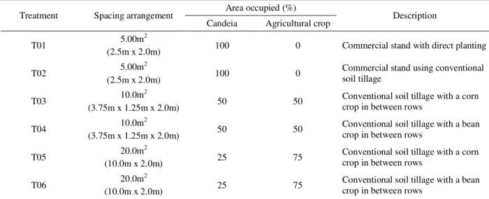
The experiment was set up in January 2005 in an area of 3.2 ha, using a randomized block design consisting of six treatments (Table 1) of 1,500 m2 (50m x 30m) each, with three replicates.
Table 1 – Treatment characterization. Tabela 1 – Caracterização dos tratamentos.
Figure 1 provides a layout for the various treatments, where dark gray depicts hedge seedlings, light gray depicts actually usable seedlings, and white depicts agricultural crops (treatments 3, 4, 5 and 6).
In this study, a 10 year rotation cycle is being considered for candeia, since, according to Silva (2009), at that age plants have reached a minimum diameter of 8.0cm and are thus ready for use in the manufacture of fence posts and, or, oil production.
In treatments 1 and 2, clearcutting will be done at age 10 years, followed by natural regeneration over the entire treatment area, then second and remaining rotations, only with natural regeneration rather than more planting.
As for treatments 3, 4, 5, and 6, the planting of candeia seedlings and agricultural crops was done in year 0 (January 2005), deriving the first crop of corn and beans. The agricultural crop was repeated annually until halfway through the candeia cycle (year 5). In that year, after harvesting the agricultural crops, the area was prepared to receive seeds from planted candeia, establishing a natural regeneration. After harvesting the planted candeia, when they reach ten years, the area will be prepared to receive seeds from natural regeneration, establishing a second natural regeneration. From there on, every five years, there will be harvest of candeia in one portion of the area, subsequently preparing the area for receiving seeds.
2.2 Dendrometric variables
Ever y six mon th s from establish in g th e experiment, each stem was measured so as to obtain diameter 1.30m above ground level (DAP) and total height. This information was used for computing volume per tree and volume per hectare, using the volume equation fitted by Scolforo et al. (2008) while studyin g candeia in Aiur uoca/MG, where: ln(VTCC)=0+1*ln(DAP2*Ht). With volume output
data obtained semiannually, timber output was estimated considering a rotation of 10 years.
It was not possible to estimate or quantify the volume output from regenerated candeia, in which case the volume output from planted candeia was assumed to be equivalent.
2.3 Model development for economic analysis
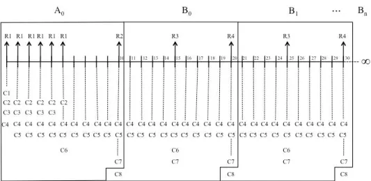
For analysis of economic feasibility, a flowchart was prepared (Figure 2) illustrating the cash flow of the agroforestry system. The rotation cycles were divided into ‘A’, referring to the cycle of candeia derived from seedlings, and ‘B’, referring to the cycle derived from regeneration, repeated over time.
For Treatments 1 and 2, in which only candeia was planted, production cost was considered to include: planting (C2), manual weeding (C3), ant control (C4), harvest (C6) and regeneration management (C7) in the rotation year. Treatment Spacing arrangement Area occupied (%) Description
Candeia Agricultural crop
T01 5.00m
2
(2.5m x 2.0m) 100 0 Commercial stand with direct planting
T02 5.00m
2
(2.5m x 2.0m) 100 0
Commercial stand using conventional soil tillage
T03 10.0m
2
(3.75m x 1.25m x 2.0m) 50 50
Conventional soil tillage with a corn crop in between rows
T04 10.0m
2
(3.75m x 1.25m x 2.0m) 50 50
Conventional soil tillage with a bean crop in between rows
T05 20.0m
2
(10.0m x 2.0m) 25 75
Conventional soil tillage with a corn crop in between rows
T06 20.0m
2
(10.0m x 2.0m) 25 75
Figure 1 – Graphic representation of experimental treatments. Figura 1 – Esquema dos tratamentos do experimento da candeia.
Where: A – 1st rotation cycle of planted candeia; B – successive rotation cycles of regenerated candeia; R1 – revenue from agricultural crop; R2 – revenue from planted candeia; R3 – revenue from candeia regenerated in the agricultural crop area; R4 – revenue from candeia regenerated in the planted candeia area; C1 – cost of agricultural crop; C2 – cost of planting candeia; C3 – cost of weeding candeia; C4 – cost of ant control; C5 – cost of land; C6 – cost of managing candeia regeneration in the agricultural crop area; C7 – cost of harvest and transportation of candeia; C8 – cost of managing regeneration in the planted candeia area.
Figure 2 – Cash flow illustrating incomes and costs, irrespective of treatment.
Revenue was considered to be the income derived from sale of clearcut timber (R2 and R4). It should be noted that for treatment T01 there were no soil tillage and liming costs.
In treatments 3, 4, 5 and 6, in which candeia was intercropped with other agricultural crops, all flowchart costs and revenues were computed. In treatments 3 and 4, 50% of the area was occupied with candeia and 50% with agricultural crops. In treatments 5 and 6, 25% of the area was destined for candeia and the remainder, 75%, was destined for agricultural crops. In year five, natural regeneration was conducted in the agricultural crop areas, thereby allowing the entire area to form a candeia stand to be managed as if it were a native candeia fragment.
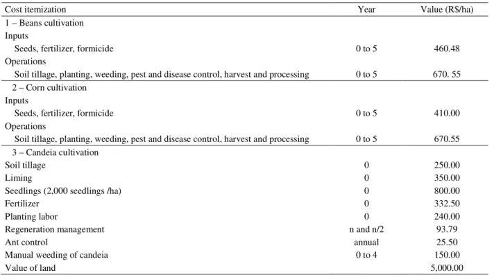
Table 2 provides costs incurred with agroforestry system activities.
2.4 Identification of Risks and Uncertainties (Input variables)
In order to conduct risk analysis for a project, it is necessary to identify opportunities and threats affecting the relevant variables. Threats potentially affecting the
economic feasibility of a project include: climate (rain and drought), forest fires, shortage of skilled labor, rework, delayed delivery by suppliers, incompatibility between project planning and its actual implementation, outdated specification of cash flow, change in scope etc. Likewise, opportunities involving an agroforestry system include: selecting higher yielding genetic material, cost lower than predicted, sale price higher than predicted, launch of cheaper, more efficient alternative materials (COELHO JÚNIOR et al., 2008).
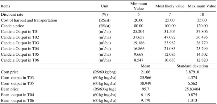
Independent variables, considered as input variables (inputs), include discount rate, cost of harvest and transportation, unit prices and the outpus of candeia, corn and beans (Table 3).
Average prices and outputs of agricultural products used here were based on historical series published by the State Department of Agriculture, Livestock and Supply of Minas Gerais state (MINAS GERAIS, 2011).
The minimum attractiveness rate adopted for the project was based on the SELIC rate less inflation for the period between January 2007 and December 2008, available at IPEADATA (www.ipeadata.gov.br).
Table 2 – Costs of agroforestry system activities.
Tabela 2 – Custos das atividades do sistema agroflorestal.
Cost itemization Year Value (R$/ha)
1 – Beans cultivation Inputs
Seeds, fertilizer, formicide 0 to 5 460.48
Operations
Soil tillage, planting, weeding, pest and disease control, harvest and processing 0 to 5 670. 55 2 – Corn cultivation
Inputs
Seeds, fertilizer, formicide 0 to 5 410.00
Operations
Soil tillage, planting, weeding, pest and disease control, harvest and processing 0 to 5 670.55 3 – Candeia cultivation
Soil tillage 0 250.00
Liming 0 350.00
Seedlings (2,000 seedlings /ha) 0 800.00
Fertilizer 0 332.50
Planting labor 0 240.00
Regeneration management n and n/2 93.79
Ant control annual 25.50
Manual weeding of candeia 0 to 4 150.00
Table 3 – Risk variables involved in the agroforestry system. Tabela 3 – Variáveis de risco envolvidas no sistema agroflorestal.
1 Conversion factor (st/m3) = 2.67
Items Unit Minimum Value Most likely value Maximum Value
Discount rate (%) 5 7 10
Cost of harvest and transportation (R$/st) 20.00 25.00 35.00
Candeia price (R$/st) 80.00 100.00 120.00
Candeia Output in T01 (m3/ha) 25.204 31.505 37.806
Candeia Output in T02 (m3/ha) 37.657 47.072 56.486
Candeia Output in T03 (m3/ha) 19.186 23.982 28.779
Candeia Output in T04 (m3/ha) 16.866 21.083 25.299
Candeia Output in T05 (m3/ha) 9.668 12.085 14.502
Candeia Output in T06 (m3/ha) 8.547 10.683 12.820
Mean Standard deviation
Corn price (R$/60 kg bag) 21.66 3.87910
Corn output in T03 (60 kg bag /ha) 25.966 4.374
Corn output in T05 (60 kg bag /ha) 38.949 6.562
Bean price (R$/60 kg bag ) 95.7 25.83404
Bean output in T04 (60 kg bag /ha) 6.119 0.875
Bean output in T06 (60 kg bag /ha) 9.179 1.313
1
1B
A n
VPL
VPL Tn VPL
i
For outputs and sale prices of candeia timber, variations of -20% to +20% relative to the most likely value were adopted in the reckoning, considering a triangular distribution, according to Rodriguez (1987).
Most likely values for cost of harvest and transportation as well as sale prices of timber were obtained from interviews with candeia producers in southern Minas Gerais state and from managers of candeia oil companies. To assess uncertainties related to inputs, a triangular distribution was used, attributing maximum, minimum and most likely values (Table 3). This distribution was used due to lack of information on probability distributions for the random variables. This distribution enables good flexibility as to the degree of skewness, a positive characteristic for subjective estimation of the distribution.
2.5 Identification of Analysis Variables or Output Variables
Net Present Value over an infinite planning horizon (VPL) was the parameter used for analyzing the various experimental treatments, according to Figure 2 flowchart. The formula used for calculating VPL is as follows:
where,
Tn= Treatment involved;
VPLA = Net Present Value of the rotation cycle of candeia derived from seedlings;
VPLB = Net Present Value of the rotation cycle of regenerated candeia;
i = Annual interest rate;
n = Duration of rotation cycle, in years.
The VPLof different management regimes was computed as output variable (outputs).
2.6 Simulation and Model Analysis
A risk analysis was done using software @Risk (PALISADE CORPORATION, 1995). According to Bentes-Gana (2003), this program enables applying the Monte Carlo method to simulate values for the random and independent variables (revenue and cost) and as a result, for the dependent variable ‘profit’.
After assembling the cash flow, 10,000 simulations were run for the output variable (VPL) using pseudorandom numbers, in other words, a series of values was generated for this analysis variable so as to obtain its simple and cumulative frequency distribution.
and taking into account other important aspects of the project.
3 RESULTS AND DISCUSSIONS
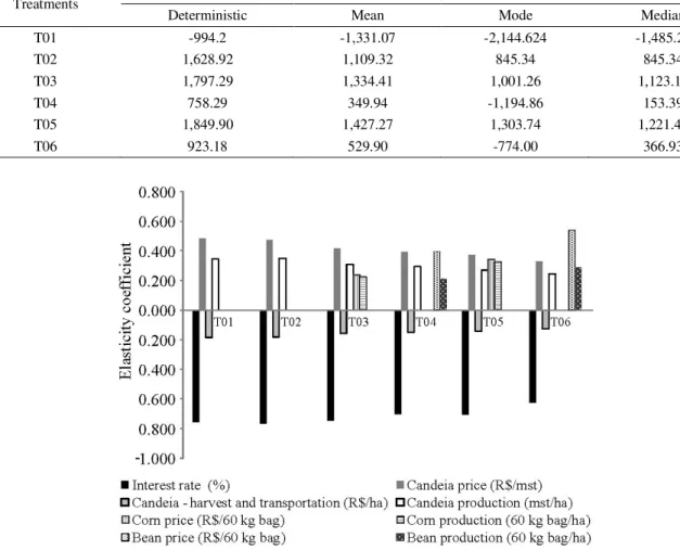
Table 4 demonstrates that, if the analysis of economic feasibility is based on VPL values calculated without computing the risks related to candeia cultivation in agroforestry systems (deterministic VPL), all treatments are economically feasible, except for Treatment 1 (T01). Treatment 5 (T05) had best financial performance, with a VPL of R$1,849.90ha-1, yet not too far from treatments 2 and 3.
Measures of position (mean, mode and median) guide as to the position of the distribution of VPL values obtained with Monte Carlo simulation, relative to the horizontal axis of the frequency curve graph. Table 4 data suggests the distribution is positively skewed, with mean values higher than median values.
Deterministic VPL values for the various treatments are higher than the values of measures of position, that is, positioned to the right of these measures in the frequency curve, suggesting overestimation.
Figure 3 provides the correlation of input variables for configuring the probability distribution of VPLin the
Table 4 – Deterministic VPL and measures of position of the interactions done in VPL simulation for different treatments. Tabela 4 – VPL em condição determinística e as medidas de posição das interações realizadas na simulação do VPL para os diferentes tratamentos.
Treatments VPL∞
Deterministic Mean Mode Median
T01 -994.2 -1,331.07 -2,144.624 -1,485.25
T02 1,628.92 1,109.32 845.34 845.34
T03 1,797.29 1,334.41 1,001.26 1,123.12
T04 758.29 349.94 -1,194.86 153.39
T05 1,849.90 1,427.27 1,303.74 1,221.48
T06 923.18 529.90 -774.00 366.93
Figure 3 – Correlation of variables resulting from the Monte Carlo simulation for the VPL of each treatment.
various treatments. The VPL of treatments 1 and 2 is influenced by interest rate and by candeia-related variables. Treatments 3, 4, 5 and 6 are also influenced by price and output of agricultural products (corn and beans).
The correlation of output and price of the various products with VPL is positive, while the correlation of this economic indicator with interest rate and with cost of harvesting and transporting candeia is negative. For example, in treatment 1, a - 0.757 correlation coefficient of interest rate indicates that a 10% increase in this variable leads to a 7.57% reduction in VPL. On the other hand, a
0.444 correlation coefficient of timber price indicates that a 10% increase in this variable leads to a 4.44% increase in VPL.
In treatment 5, correlations of price with corn output are higher than in treatment 3. This is because in treatment 5 the area occupied by the corn crop exceeds the area in treatment 3. In treatments 4 and 6 this situation is repeated with the bean crop.
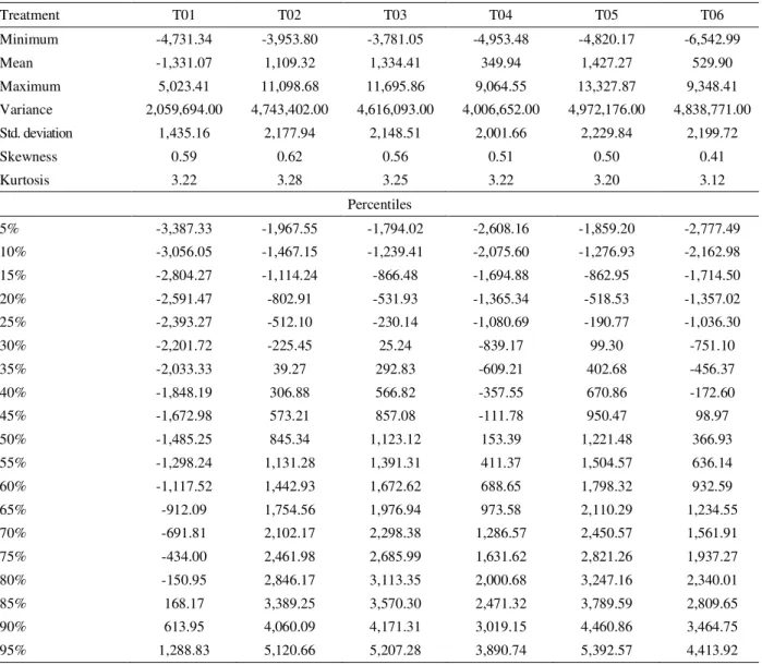
Table 5 provides VPLresults using the Monte Carlo simulation, based on variation in input data (inputs). The skewness value greater than zero for all treatments
Table 5 – Coefficients and percentiles of the output variable (VPL) for each treatment. Tabela 5 – Coeficientes e percentis da variável de saída (VPL) para cada tratamento.
Treatment T01 T02 T03 T04 T05 T06
Minimum -4,731.34 -3,953.80 -3,781.05 -4,953.48 -4,820.17 -6,542.99
Mean -1,331.07 1,109.32 1,334.41 349.94 1,427.27 529.90
Maximum 5,023.41 11,098.68 11,695.86 9,064.55 13,327.87 9,348.41 Variance 2,059,694.00 4,743,402.00 4,616,093.00 4,006,652.00 4,972,176.00 4,838,771.00 Std. deviation 1,435.16 2,177.94 2,148.51 2,001.66 2,229.84 2,199.72
Skewness 0.59 0.62 0.56 0.51 0.50 0.41
Kurtosis 3.22 3.28 3.25 3.22 3.20 3.12
Percentiles
5% -3,387.33 -1,967.55 -1,794.02 -2,608.16 -1,859.20 -2,777.49
10% -3,056.05 -1,467.15 -1,239.41 -2,075.60 -1,276.93 -2,162.98
15% -2,804.27 -1,114.24 -866.48 -1,694.88 -862.95 -1,714.50
20% -2,591.47 -802.91 -531.93 -1,365.34 -518.53 -1,357.02
25% -2,393.27 -512.10 -230.14 -1,080.69 -190.77 -1,036.30
30% -2,201.72 -225.45 25.24 -839.17 99.30 -751.10
35% -2,033.33 39.27 292.83 -609.21 402.68 -456.37
40% -1,848.19 306.88 566.82 -357.55 670.86 -172.60
45% -1,672.98 573.21 857.08 -111.78 950.47 98.97
50% -1,485.25 845.34 1,123.12 153.39 1,221.48 366.93
55% -1,298.24 1,131.28 1,391.31 411.37 1,504.57 636.14
60% -1,117.52 1,442.93 1,672.62 688.65 1,798.32 932.59
65% -912.09 1,754.56 1,976.94 973.58 2,110.29 1,234.55
70% -691.81 2,102.17 2,298.38 1,286.57 2,450.57 1,561.91
75% -434.00 2,461.98 2,685.99 1,631.62 2,821.26 1,937.27
80% -150.95 2,846.17 3,113.35 2,000.68 3,247.16 2,340.01
85% 168.17 3,389.25 3,570.30 2,471.32 3,789.59 2,809.65
90% 613.95 4,060.09 4,171.31 3,019.15 4,460.86 3,464.75
indicates that the distribution is skewed to the right. Kurtosis values higher than 3 indicate that the frequency distribution is more sharply peaked and concentrated than the normal distribution, characterizing a leptokurtic probability function.
From the analysis of percentiles, it is inferred that treatment 1 has the highest probability of negative VPL occurring (80% to 85%). In treatments 3 and 5, the probability of a negative VPL occurring is lower, 30% to 35%.
Treatments 3 and 5 had the highest VPL values, with a slight advantage to treatment 5. Further analysis of these treatments, based on Table 5 statistics, indicates that the risk related to these treatments is very close. It can be noted that the expected (mean) VPL of T05 is R$ 1,427.27, with a standard deviation of R$ 2,229.84. Therefore, with 0.64 standard deviations, a zero VPL is attained. Likewise, T03 requires 0.62 standard deviations for a zero VPL.
The mean VPLor expected VPL calculated with risks being taken into account (Table 5) is always less than the VPL calculated without risks being taken into account (deterministic analysis) (Table 4). In treatment 5, for instance, with risks being considered, the mean value of this parameter is R$ 1,427.27. In the deterministic analysis, however, the VPL is R$ 1,849.90.
According to Table 5 percentiles, there is a 35% to 40% probability that the deterministic VPLof treatment 1 (-R$ 994.20) (Table 4) will occur or be surpassed. The probability range of this happening for the other treatments is the same, except for treatment 6, where the range is 40% to 45%.
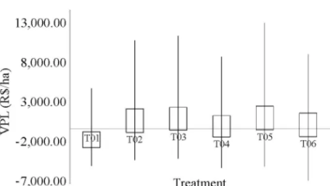
Figure 4 provides the range of VPL values with a 90% confidence interval, that is, ignoring 5% above and 5% below the distribution. For each treatment, VPL values were divided into three scenarios: a most likely scenario depicted by rectangles, an optimistic scenario depicted by the line above the rectangles indicating the data range, and a pessimistic scenario depicted by the line below the rectangle. According to Castro et al. (2007), the pessimistic scenario occurs when costs are high while prices and output are low, making the project economically unfeasible. With a deterministic analysis it would not be possible to infer about the possibility of projects being economically unfeasible, as it does not consider variable randomness.
Regarding the most likely scenario, treatment 1 (T01) is economically unfeasible, since all VPLvalues are negative in the data range that expresses this scenario. In treatments where candeia is intercropped with corn (T03 and T05), the risk is lower, since few VPLvalues are negative in the most likely scenario.
Figure 4 – Distribution of output variables resulting from the Monte Carlo simulation for the VPL” of each treatment. Figura 4 – Distribuição das variáveis de saída resultantes da simulação de Monte Carlo para o VPL” de cada tratamento.
4 CONCLUSIONS
The agroforestry systems being tested are economically feasible, noting that the system in which candeia is cultivated at spacing intervals of 10 x 2 meters, intercropped with corn in between rows, is more profitable and less risky than the others.
Candeia cultivation as a monoculture is economically feasible, provided that soil tillage is done conventionally.
5 REFERENCES
BENTES-GANA, M. M.; SILVA, M. L.; VILCAHUMÁN, L. J. M.; LOCATELLI, M. Análise econômica de sistemas agroflorestais na Amazônia ocidental, Machadinho D’Oeste, RO. Revista Árvore, Viçosa, v. 29, n. 3, p. 401-411, maio/jun. 2005.
BUDOWSKI, G. Aplicabilidad de los sistemas agroflorestais. In:SEMINÁRIO SOBRE PLANEJAMENTO DE
PROJETOS AUTO-SUSTENTÁVEIS DE LENHA PARA AMÉRICA LATINA E CARIBE, 1991, Turrialba. Anais...
Turrialba: FAO, 1991. v. 1, p. 161-167.
CASTRO, R. R.; SILVA, M. L.; LEITE, H. G.; OLIVEIRA, M. L. R. Rentabilidade econômica e risco na produção de carvão vegetal. Cerne, Lavras, v. 13, n. 4, p. 353-359, out./dez. 2007.
COELHO JÚNIOR, L. M.; REZENDE, J. L. P.; OLIVEIRA, A. D.; BORGES, L. A. C.; SOUZA, A. N. Análise de
investimento de um sistema agroflorestal sob situação de risco.
DIXIT, A. K.; PINDICK, R. S. Investment under uncertainty. Princenton: Princeton University, 1994. 468 p.
DUBOIS, J. C. L. Manual agroflorestal para a Amazônia. Rio de Janeiro: Rebraf, 1996. v. 1, 228 p.
MINAS GERAIS. Secretaria de Estado de Agricultura, Pecuária e Abastecimento de Minas Gerais. Disponível em: <http://www.agricultura.mg.gov.br/>. Acesso em: 10 maio 2011.
RAMÍREZ, G. A. et al. Financial returns, stability and risk of cacao-plantain-timber agroforestry systems in Central America. Agroforestry Systems, Wageningen, v. 51, n. 1, p. 144-154, 2001.
RODRIGUEZ, L. C. E. Planejamento agropecuário através de um modelo de programação linear não determinista. 1987. 83 p. Dissertação (Mestrado em
Economia Agrária) - Escola Superior de Agricultura “Luiz de Queiroz”, Piracicaba, 1987.
SCOLFORO, J. R. S. et al. Volume, peso de matéria seca e produção de óleo para candeia (Eremanthus erythropappus), em Minas Gerais. In: SCOLFORO, J. R. S.; OLIVEIRA, A. D.; ACERBI JÚNIOR, F. W. (Ed.). Inventário florestal de Minas Gerais: equações de volume, peso de matéria seca e carbono para diferentes fitofisionomias da flora nativa. Lavras: UFLA, 2008. p. 171-179.
SECURATO, J. R. Decisões financeiras em condições de risco. 2. ed. São Paulo: Ed. Saint Paul, 2007. 264 p.
SHIMIZU, T. Pesquisa operacional em engenharia, economia e administração: modelos básicos e métodos computacionais. Rio de Janeiro: Guanabara Dois, 1984. 360 p.