COSMIC RAY GROUND LEVEL ENHANCEMENTS (GLEs) OF OCTOBER 28, 2003
AND JANUARY 20, 2005: A SIMPLE COMPARISON
Rajaram Purushottam Kane
Recebido em 10 setembro, 2008 / Aceito em 27 abril, 2009 Received on September 10, 2008 / Accepted on April 27, 2009
ABSTRACT.The evolutions of the Ground Level Enhancements (GLEs) of Oct. 28, 2003 (the famous Halloween event) and the subsequent Jan. 20, 2005 (a very large event in the declining phase of cycle 23) were examined. It was noticed that the Oct. 28, 2003 GLE was a very small one, in contrast to the large CR Forbush decreases and geomagnetic Dst storms that occurred the next day, on Oct. 29, 2003. These may not have the same origins. Hence, three more events were also studied, namely the largest GLE 5 of Feb. 23, 1956 (meager data), the second largest GLE 42 of Sep. 29, 1989, and the fourth largest GLE 45 of Oct. 24, 1989 (comparable to GLE 69, the third largest GLE of Jan. 20, 2005). For each, the plots of few-minute and/or hourly values as also the latitude-longitude distributions of the GLE magnitudes (percentage increases) were examined. It was noticed that at similar mid-latitudes, locations at different longitudes showed different latitude distributions of the magnitudes, indicating that events had longitudinal anisotropies, more in some events, less in others. Thus, the present paper illustrates a simple way of detecting anisotropies qualitatively. Only the maximum enhancement magnitudes were used, irrespective of the phases (maxima occurring at different times at different locations). If simultaneous magnitudes are used as these occurred at specific UTs in succession, more details could be studied such as changes in the characteristics (spectra etc., or multiple populations) of the incoming particles, as is done in sophisticated analyses. The present approach may be considered as a first look at a complex phenomenon. Keywords: cosmic rays, ground level enhancements, GLEs.
RESUMO.A evoluc¸˜ao do aumento de raios c´osmicos na superf´ıcie terrestre (GLE) no dia 28 de outubro de 2003 (evento Halloween) e outro evento subseq¨uente no dia 20 de janeiro de 2005 (um evento grande em fase de decl´ınio da atividade solar) foram examinados. O GLE no dia 28 de outubro foi notado pequeno, por´em a diminuic¸˜ao Forbush e o ´ındice Dst no dia seguinte foram grandes. Origens podem ser diferentes. Por isso, trˆes eventos foram estudados, evento no dia 23 de fevereiro de 1956 (poucos dados), segundo evento de 29 de setembro de 1989 e de 24 de outubro de 1989. Para cada evento foram examinados gr´aficos de alguns minutos e/ou valores m´edios hor´arios como tamb´em distribuic¸˜ao latitudinal e longitudinal das magnitudes de eventos GLEs. Foi observado nas latitudes m´edias e similares que a variac¸˜ao latitudinal nas longitudes diferentes ´e distinta indicando que os eventos tˆem anisotropia longitudinal, mais em alguns eventos e menos em outros. O presente trabalho demonstra de maneira simples e qualitativamente via ilustrac¸˜oes das anisotropias. Somente as amplitudes m´aximas foram usadas independente de suas fases, usando magnitudes simultˆaneas porque os eventos ocorreram nos espec´ıficos tempos UT em sucess˜ao. Mais detalhes como as caracter´ısticas (espec-tros etc. ou populac¸˜oes m´ultiplas) podem ser estudados sobre as part´ıculas que entram, atrav´es de an´alises sofisticadas. Este trabalho pode ser considerado como a primeira vis˜ao de um fenˆomeno complexo.
Palavras-chave: raios c´osmicos, aumento da superf´ıcie terrestre, GLE.
Instituto Nacional de Pesquisas Espaciais, INPE, Caixa Postal 515, 12245-970 S˜ao Jos´e dos Campos, SP, Brazil. Phone: +55(12) 3945-6795; Fax: +55(12) 3945-6810 – E-mail: [email protected]
INTRODUCTION
One of the most spectacular solar phenomena is the Solar Flare, which is observed in the solar chromosphere, with a sudden release of very large amounts of energy. Solar flares produce electromagnetic emissions, accelerate electrons and ions and under favorable conditions, inject these into interplanetary space. There are two broad mechanisms, impulsive mechanisms that may have several stages, and acceleration mechanisms based on the passage of shock waves through the corona. The injec-tion of energetic particles in space is termed in general as a SEP (solar energetic particle) event, or specifically, a SPE (solar pro-ton event). Though it is often associated with large solar flares, sometimes, the association is with a disappearing filament with-out any accompanying flare (Kahler et al., 1986; Smart & Shea, 1989). The particles have a large spread of energies and reach the Earth’s orbit (1 AU) with a delay of a few tens of minutes to seve-ral hours. In earlier years, the SEP events were detected mainly by cosmic ray monitors (ionization chambers, meson telescopes, neutron monitors) which yielded very limited information; but with the advent of satellites, the information obtained is much larger. The events observed by instruments on the ground are termed GLEs (Ground Level Enhancements). The onset time and the ma-ximum intensity of the solar particle flux depend on the heliolon-gitude of the flare with respect to the detection location in space. Particles move more easily along the interplanetary magnetic fi-eld lines, whose topology is determined by the solar wind outflow and the rotation of the Sun (approximately Archimedean spiral). The propagation of solar protons from the flare site to the Earth has two independent phases: (1) diffusion in the solar corona and (2) transport into the heliosphere along the interplanetary field li-nes. Assuming that the maximum flux occurs at the solar flare site, there would be a gradient extending into the corona from the solar flare site to other heliolongitudes. Spacecraft obser-vations of solar particles have indicated such gradients, though the magnitudes vary from event to event (detailed references in Smart & Shea, 1989).
Using data from different satellites, considerable details about the nature of SEPs (Solar energetic particles) and their non-uniform evolutions in time during the same event have been ob-tained (see review by Ryan et al., 2000). In conjunction with simultaneous data for other radiations (X-rays, Gamma rays, e.g., Kuznetsov et al., 2005). These are useful for modeling of solar flares.
GLEs are sharp increases in the ground-level cosmic ray count to at least 10 percent above background, associated
with solar protons of energies greater than 500 MeV, and are relatively rare, occurring only a few times each solar cycle. When they occur, GLEs begin a few minutes after flare maximum and last for a few tens of minutes to hours. Intense particle flu-xes at lower energies can be expected to follow this initial burst of relativistic particles. GLEs can be detected by cosmic ray neutron and meson monitors. Peg Shea (Emeritus, U.S. Air Force Re-search Labs. AFRL) has been compiling these events and num-bering them, with Event 1 = 28 Feb. 1942, Event 63 = 26 Dec. 2001, and so on. Several individual events have been studied in detail so far (e.g., August 1972 events by Rao, 1976; the 1989 events by Reeves et al., 1992 and Lovell et al., 1998; July 14, 2000 event by Belov et al., 2005, etc.). Information about GLEs collected so far is of two types, namely the physical as-pects (time profiles, spectra etc., e.g., Shea & Smart, 1996) and statistical aspects (occurrence frequency etc.). Summarizing the results of 40 years data, Shea & Smart (1990), stated that other than an increase in solar proton event occurrence with increasing solar cycle, no recognizable pattern could be identified between the occurrence of solar proton events and the solar cycle. In a recent publication, Shea & Smart (2001a) mention that the num-ber of >10 MeV solar proton events with peak flux exceeding 10/cm2-sec-ster) during each solar cycle was remarkably cons-tant for solar cycles 19-22, even though the total integrated flu-ence experiflu-enced at the Earth per solar cycle varied by a factor of four. In addition, the number of ground level enhancements each solar cycle also remained relatively constant. From the si-milarities between the first five years of solar cycle 23 and the first five years of solar cycle 20, they expected the majority of solar proton events to occur during years 5-8 of the 23rdcycle (i.e. during 2000-2004) with perhaps a surge of activity during the waning years of the cycle. This expectation has come true. The 12-monthly average sunspot activity peaked around 120 du-ring July 2000-February 2002 and declined thereafter to reach about half the peak value by the end of 2003, but the interval October-November 2003 (Halloween events) was marked by a very strong solar flare activity. (The Dst storm of November 20, 2003 was the second largest in recorded history, only second to the largest Dst storm of March 13, 1989). Further, on Janu-ary 20, 2005 when sunspot activity was almost one-third of the peak value, a ground level enhancement occurred, which is men-tioned by some workers (discussed later) as second largest in recorded history, i.e., only second to the GLE of February 23, 1956. The GLEs of October 28, 2003 and January 20, 2005 have received great attention from the scientific community and the event of 2005 was so spectacular that within a few months,
several studies were reported at the 29th International Cosmic Ray Conference (ICRC August 2005) at Pune, India, for indivi-dual locations or for a group of locations (Bieber et al., 2005a,b; Fl¨uckiger et al., 2005; Miyasaka et al., 2005; Moraal et al., 2005; S´aiz et al., 2005; Timofeev et al., 2005; Vashenyuk et al., 2005a,b,c; Zhu et al., 2005). The studies of these two events were about various aspects such as, time profiles (including anisotro-pies at different phases of evolution), ionic charge state compo-sitions (Labrador et al., 2005) and spectra (e.g., Mewaldt et al., 2005), probable relationships with specific flares and their evo-lution phases, with CMEs and ICME shocks etc., and even pos-sibility of arrival of high energy neutrons (Bieber et al., 2005a; Struminsky, 2005a). For GLE studies, the interpretation of the magnitudes of increases needs information about the vertical cut-off rigidities, which seem to have changed with time due to se-cular changes in geomagnetic field (Shea & Smart, 2001b), res-ponse functions of the neutron monitors (including angle de-pendent yield functions, e.g., Clem & Dorman, 2000), as also about the asymptotic coordinates due to deflection in geomag-netic field (e.g., Tsyganenko, 1989). All these can be used for a theoretical modeling of the transport of solar material (e.g., Fedorov et al., 2002) up to the cosmic ray detectors. Apart from unusual intensity profiles and anisotropies generally in the initial phase of a GLE (e.g., Shea & Smart, 1996), statisti-cal studies are reported, which have indicated arrival of parti-cles along the IMF (interplanetary magnetic field) lines, though some discrepancies are often seen (Belov et al., 2001, 2005). Miroshnichenko et al. (2005) reported particle arrival from the anti-sunward direction also. For spectra, the neutron monitor data are not very useful as these are in the comparatively high energy tail of a SPE. Satellite data for very low energy parti-cles (protons as well as heavier ions, Cohen et al., 2005) are the most useful and often show double-power law formalism (Mewaldt et al., 2005; Struminsky, 2005b). Gopalswamy et al. (2005) reported that GLE-associated CMEs represented the fas-test known population of CMEs and all the GLEs were associa-ted with metric Type II bursts, and particle acceleration occurred in CME-driven shocks before GLEs were released from the Sun (apparently, in disagreement with Simnett, 2006).
Since the arrival direction is from sunward, the anisotropies should show as longitudinal phase differences for similar lati-tudes. The GLE phenomenon can be studied and is studied in a very sophisticated way (geomagnetic bending, energy depen-dence, pitch angle distribution, etc.) by several workers for se-veral individual events. However, in the present communication, the intensity-time profiles and the latitude-longitude
distributi-ons of the magnitudes of the increases are examined in a simple qualitative way for the two GLEs of October 28, 2003 and Janu-ary 20, 2005. So, sophistications are mentioned in the text but not used for analysis.
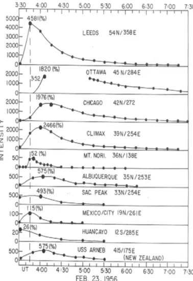
Figure 1 – Plots of neutron monitor count rates at ten locations (names and latitude-longitude indicated) during 03:30-07:30 UT of Feb. 23, 1956. The big dots indicate the maxima (percentage value indicated).
DATA PLOTS
Neutron monitor data were obtained mostly from the NOAA website (SPIDR), though some were obtained privately. On the occasion of the 50thanniversary of the famous Feb. 23, 1956 GLE event (Meyer et al., 1956), it may be interesting for the modern generation to have a look at the intensity-time plot of this event. The event was so strong that even meson telescopes in India showed increases of a few percent (Sarabhai et al., 1956; Kane & Ahluwalia, 1957). For that occasion, H.E. Elliot and T. Gold prepared a document entitled “Collection of cosmic ray, solar, ionospheric and magnetic data relating to the solar cosmic ray burst of 23rd February 1956” (unpublished) wherein Forbush mentions a few percent increases in ionization chamber records (see also Forbush, 1946 for earlier events and Duggal, 1979). Figure 1 shows the plots for 10 neutron monitors which were
operative during this interval. Note that data for some vital high latitude monitors (Thule, McMurdo, South Pole) are missing, as these started operating only one year later (1957). (A similar fi-gure but with all datasuperimposed is given as Figure 1 in the FINAL REPORT NAG54011, “Ground-Level Solar Cosmic Ray Data from Solar Cycle 19” Period of Performance: 1 January 1999-30 March 2002, by M.A. Shea, PI, University of Alabama, Huntsville, AL 35899). The following may be noted:
(1) There is only one high latitude location (Leeds, in UK, 54◦N) It showed an enormous increase of 4581% (in 15 min.). Other large increases were at Ottawa (45◦, 1820%, 1-min.), Chicago (42◦, 1976% in 15 min.), Climax (39◦, 2466% in 15 min.) in American longitudes; but these in-creases are only about half of those of Leeds. This reduc-tion could be due to lower latitudes or longitudinal ani-sotropies. Albuquerque (35◦, 575%, in 15 min.), Sacra-mento Peak (33◦, 493% in 30 min.), Mexico City (19◦, 115% in 15 min) and Huancayo (12◦, 26% in 30 min), all in the American longitudes, do indicate a strong latitude effect (reduction at lower latitudes).
(2) Figure 2 shows a plot of the magnitudes (ordinate, log scale)versus latitude (North and South mixed together) for locations in the American longitudes (dots), Leeds in UK (triangle) and Mt. Norikura and the shipboard instru-ment USS Arneb (anchored at Wellington coast in New Zealand) as open circles. If a straight line is drawn as shown, all American longitudes and Leeds fall on or near the straight line, while Mt. Norikura and USS Arneb are below the line, indicating that the GLE event occurred fa-vorably for the European-American longitudes (0-90◦W) but unfavorably for far-East longitudes.
(3) The observations are mostly for 15-minute intervals, but for Ottawa, 1-min values were available and these show a start of the GLE at 03:52 UT. The maximum could have occurred at 4:05 UT but the data were interrupted thereaf-ter. However, these timings do not seem to be the same at all locations, where the intensities were at zero level at 3:30 UT but were already high at 3:45 UT (vertical dashed line). For Leeds (0◦E), Mt. Norikura (138◦E) and Mexico City (261◦E), the maximum was near 3:45 UT, for Huan-cayo (285◦E), it was earlier (even at 3:30 UT), while for others (Ottawa 284◦E, Chicago 272◦E, Climax 254◦E, Al-buquerque 253◦E, Sacramento Peak 254◦E, USS Arneb 175◦E), the maxima were ∼15 minutes later, near 4:00 UT. Thus, in these limited data, no clear longitude effect
is seen, and precipitation could be partly erratic (even al-lowing for geomagnetic bending). It should be noted that the incoming particle radiation has a very wide spectrum and lower energy particles suffer larger geomagnetic de-flections.
Figure 2 – Maximum magnitude (ordinate, log scale)versuslatitude, for the ten neutron monitors which recorded the event of Feb. 23, 1956.
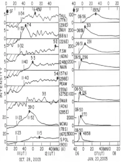
Let us now have a look at the events of Oct. 28, 2003 and Jan. 20, 2005. The SPIDR website gave data only for hourly values. However, John Bieber and Roger Pyle of the Bartol Research Ins-titute kindly supplied us 1-minute data for these events for their eight neutron monitors. These are plotted in Figure 3, for the Oct. 28, 2003 event on the left side and the Jan. 20, 2005 event on the right side. The following may be noted:
(A) Event of Oct. 28, 2003: A solar flare (indicated by a big full circle) started at ∼11:00 UT. The GLE had increa-ses of 3-7% in the northern hemisphere, starting between 11:32 and 11:40 UT, but with maximum at widely diffe-rent times, some occurring even in the next hour (Fort Smith, 12:50 UT). However, magnitudes were much lar-ger in the southern polar region (McMurdo 39%, South Pole 11.5%), indicating an overwhelming preference for precipitation in the southern hemisphere, but mainly near the poles. At McMurdo, the event lasted for only ∼70 mi-nutes (peak at 11:52 UT), but at other locations (including the South Pole), it lasted for more than an hour (several hours as shown later). Thus, even in a small region near the South Pole, precipitation was qualitatively and quanti-tatively different.
(B) Event of Jan. 20, 2005: A solar flare (indicated by a big full circle) started at ∼06:40 UT. This event had increases
several tens to hundreds of times larger than those in the Oct. 28, 2003 event, all starting at ∼6:50 UT. The event
was short-lived (rise time <10 minutes, but Thule had a long rise time of 35 minutes). Increases were 100-300% in the northern hemisphere. However, magnitudes were enor-mous in the southern polar region, (McMurdo 2700%, South Pole 4860%, in 3 min), indicating an overwhelming preference for precipitation in the southern hemisphere. In this case, the evolution near the South Pole region was at least qualitatively similar.
Figure 3 – Plots of the 1-minute values of the count rates of eight neutron mo-nitors (names and latitude-longitude indicated) operated by the Bartol Research Institute, University of Delaware (data courtesy John W. Bieber and Roger Pyle). The big dots indicate the maxima (percentage value indicated). Other numbers indicate time in UT.
The large magnitudes in 2005 cannot be compared directly with those of the Feb. 23, 1956 event, because none of these eight neutron monitors of the Bartol Research Institute were operative in 1956, while Leeds, having the largest increase in 1956, was not operative in 2005. Climax is the only middle latitude monitor operative in 1956 as well as 2005. In 1956, Climax values were available for 15-minute intervals and showed a maximum value of 2466%. If hourly values are calculated, the maximum hourly va-lue in 1956 for Climax was 1837%, much larger than the 36% for 2005. Thus, the 1956 event was probably very much larger than the 2005 event. This can be seen from the value for Huancayo
also, which was 26% in 1956, but only 3% in 2005 at Haleakala which replaced Huancayo in recent years.
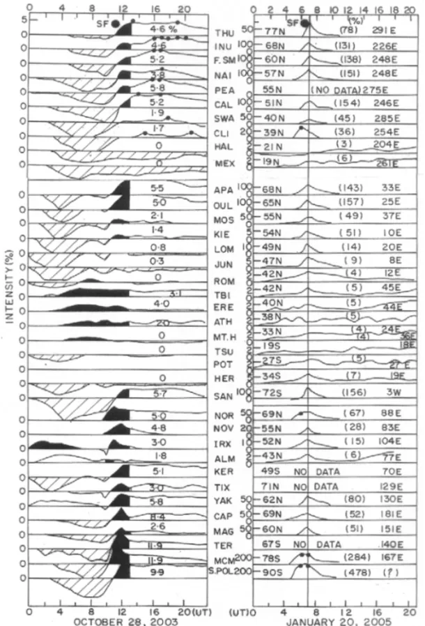
Figure 4 shows the plots of hourly values for count rates of several neutron monitors, the first ten for north-American lon-gitudes (204◦-298◦E, Thule to Mexico City in the northern he-misphere), the next fifteen for European longitudes (03◦W-45◦E, Apatity in the North to Sanae in the South), the next five for the eastern longitudes (70◦-104◦E, Norilsk in the North to Kergue-len Islands in the South), and the next seven for the far-eastern longitudes (129◦-180◦E, Tixie Bay in the North to McMurdo and South Pole in the South), with the October 28, 2003 event on the left side and the Jan. 20, 2005 event on the right side. Table 1 gives the details. The following may be noted:
(A) Event of Oct. 28, 2003: The GLE started during 11 and 12 UT, but before the event, there was a mild cosmic ray decrease (Forbush decrease?) of ∼5-10% depression, much smaller than the very large Forbush decrease that occurred next day (Oct. 29, ∼06 UT, ∼30% depression). The cosmic ray depression seems to have occurred at dif-ferent time intervals at difdif-ferent latitudes and longitudes indicating considerable anisotropies, but the depression seems to have ended just before the GLE beginning at ∼11 UT at all locations; so, no interference is expec-ted, and the GLE magnitudes are estimated as above the base level at ∼0 UT, before the cosmic ray decrease. The GLE was strong in high latitudes, hourly magnitudes ∼5% in North and ∼11% in the South, and was long-lasting, almost 7-8 hours at an almost constant level, declining slowly thereafter. (At some locations, e.g., Tbilisi and Erevan, ∼40◦N, 45◦E; Athens, 40◦N, 24◦E, there were
positivedeviations instead of the decrease in the pre-GLE interval 06-11 UT. We do not know whether this is due to data error, or the CR decrease did not occur at these loca-tions and showed instead as a CR increase).
(B) Event of Jan. 20, 2005: This was a short-lived GLE, with main increase during 06-07 UT and a rapid fall there-after. Magnitudes of hourly values were ∼80-150% in high northern latitudes (∼20-30 times larger than in the Oct. 28, 2003 event) and ∼280-480% in high southern latitudes (again ∼20-30 times larger than in the Oct. 28, 2003 event).
From Figures 3 and 4, it seems that large anisotropies oc-curred in the first 60 minutes and the evolutions were different at different locations, with durations notably longer at Thule.
Table 1 – Details of the locations of neutron monitors and the percentage increases in the GLEs 65, 69, 42 and 45 of Oct. 28, 2003; Jan. 20, 2005; Sep. 29, 1989; and Oct. 24, 1989 respectively. Vertical cut-off rigidities depend upon the geomagnetic reference field which is having a secular variation. The values mentioned are for 1995 (Shea & Smart, 2001b).
Vertical Oct. 28, 03 Jan. 20, 05 Sep. 29, 89 Oct. 24, 89 Lat. E. Long Cut-off Increase Increase Increase Increase
1995 % % % %
Thule, Greenland 76.50 291.30 0.00 4,6 78 343 86 Inuvik, Canada 68.35 226.28 0.14 4,6 131 336 92 Fort Smith, Canada 60.02 248.07 0.30 5,2 138
Nain, Canada 56.55 298.32 0.45 3,8 151 Peawanuck, Canada 54.98 274.56 0.40 5,8
Goose Bay, Canada 53.27 299.60 0.74 211 71 Calgary, Canada 51.08 245.87 1.09 5,2 154 345 103 Deep River, Canada 46.10 282.50 1.25 208 74 Mt. Washington, USA 44.30 288.70 1.58 258 107
Durham, USA 43.10 289.17 1.76 144 59
Swarthmore, USA 39.90 284.65 2.21 1,9 45 153 44 Climax, USA 39.37 253.82 2.93 1,7 36 178 40 Haleakala, USA 20.72 203.73 12.76 0,1 3,3 14 1.70 Mexico City, Mexico 19.33 260.80 8.02 0,1 5,5
Apatity, Russia 67.55 33.33 0.55 5,5 143 180 102 Oulu, Finland 65.05 25.47 0.77 5 157 164 93 Moscow, Russia 55.47 37.32 2.30 2,1 49 Kiel, Germany 54.33 10.13 2.36 1,4 51 150 44 Kiev, Ukraine 50.72 30.30 3.39 116 19 Dourbes, Belgium 50.10 04.60 3.33 113 19
Lomnicky Stit, Slovakia 49.20 20.22 3.88 0,8 14 120 20 Jungfraujoch, Switzerland 46.55 7.98 4.59 0,3 9 126 11 Rome, Italy 41.86 12.47 6.27 0,1 4,3 76 0.10 Tbilisi, Georgia 41.72 44.80 6.55 3,1 4,6 83 0.10 Erevan, Armenia 40.17 44.25 7.36 4 5,4 Athens, Greece 37.97 23.72 8.53 2,2 4,9 Mt. Hermon, Israel 33.30 35.79 10.41 0,1 4,3 Tsumeb, Namibia –19.20 17.58 9.06 0,1 4,2 40 0.10 Potchefstroom, S. Africa –26.68 27.10 6.85 5,2 80 0.10 Hermanus, S. Africa –34.42 19.22 4.45 0,1 6,6 92 8 Sanae, Antarctica –71.67 357.15 0.75 5,7 156 266 133 Norilsk, Russia 69.26 88.05 0.53 5 67 Novosibirsk, Russia 54.80 83.00 2.69 4,8 28 167 34 Irkutsk, Russia 52.47 104.03 3.49 3 15 188 18 Alma Ata, Kazakhstan 43.25 76.92 6.45 1,8 5,7 39 2 Kerguelen Islands, France –49.35 70.25 1.14 5,1 250 90
Tixie Bay, Russia 71.58 128.92 0.43 3 220 78 Yakutsk, Russia 62.03 129.73 1.55 5.8 80 257 72 Cape Schmidt, Russia 68.92 180.53 0.52 8,4 52 327 85 Magadan, Russia 60.12 151.02 1.99 2,6 51 296 58 Mt. Norikura, Japan 36.11 137.55 11.25 21 1.10
Tokyo, Japan 35.75 139.72 11.40 17 0.10
Mt. Wellington, New Zealand –42.92 147.23 1.83 324 83 Terre Adelie, Antarctica –66.65 140.01 0.00 11,9 258 119 McMurdo, Antarctica –77.85 166.72 0.00 11,9 284 262 107 South Pole, Antarctica –90.00 ? 0.05 9,9 478 346 189
Figure 4 – Plots of hourly values of neutron monitor count rates at several locations (names and latitude-longitude indicated), for the event of Oct. 28, 2003 (left half) and Jan. 20, 2005 (right half). For the Oct. 28, 2003 event, there was a CR Forbush decrease (shown hatched) during 00-11 UT The GLE started at ∼11 UT (shown partly black) and lasted for a long time. For the Jan. 20, 2005 event, the GLE started at ∼06 UT and lasted for only ∼2 hours. Numbers indicate magnitudes of the maximum increase in percentages. In the October 28, 2003 event, the evolution was different for
McMurdo and South Pole, but in the January 20, 2005 event, the evolutions were similar. In hourly values, there were proba-bly no major anisotropies, except that there was a major
North-South anisotropy, with southern polar region receiving much lar-ger flux than the northern polar region.
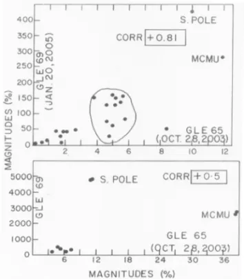
To see whether different GLEs have increases in the same pro-portions at various locations, Belov et al. (2005) plotted the GLE
peak enhancements of GLE 59 (July 14, 2000)versus those of GLE 52 (June 15, 1991) and found that these were of compa-rable magnitudes and were very well correlated (+0.97). In the present case, the magnitudes at the various locations were 20-30 times larger in the Jan. 2005 event. Figure 5 shows a plot of the maximum values of the Jan. 20, 2005 event (GLE 69, ordi-nate)versus those of the Oct. 28, 2003 event (GLE 65, abscissa). As can be seen, in the upper part where hourly values were used, the correlation is +0.81, not very large mainly because of the scatter in the middle range (marked in an oval). The slope is 29.9±3.9, indicating that the GLE 69 hourly maxima were ∼26-33 times larger than those of GLE 65. In the lower part of Figure 5, the seven points corresponding to the maximum 1-minute values of Figure 3 are shown. The correlation is only +0.51, mainly because the points for McMurdo and South Pole are far apart.
Figure 5 – Plots of the magnitudes of GLE 69 of Jan. 20, 2005 (ordinate) ver-susmagnitudes of GLE 65 of Oct. 28, 2003 (abscissa), upper half for all neutron monitors, lower half for only seven monitors of the Bartol Research Institute.
LATITUDE AND LONGITUDE EFFECTS
Figure 6 shows the approximate magnitudes of the GLE 65 (Oct. 28, 2003) at the various locations (latitudes and longitudes) by five symbols. As can be seen, all large magnitudes (big full cir-cles and squares) are at high latitudes, spread at all longitudes in the northern hemisphere (implying very little longitudinal aniso-tropy), and with larger values in the southern polar region (North-South asymmetry). (North-South Pole does not have a longitude and is shown as at 0 longitude with arrows showing its extension to other
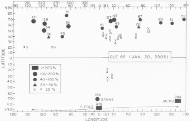
longitudes. Figure 7 shows a similar plot for GLE 69 (Jan. 20, 2005) using five symbols, but with magnitudes much larger than those in Figure 6. Here too, large values are at higher latitudes but these are mostly in the longitudes 0-90◦W, indicating considera-ble longitudinal anisotropy. Again, values in the southern polar region are higher.
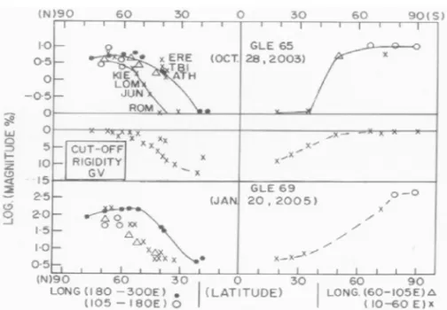
Figure 8 shows plots of percentage magnitudes of GLE in-creases (ordinate is log scale)versus latitudes of various lo-cations, with longitudes marked by different symbols (180◦ E-300◦E, full circle; 105◦E-180◦E, open circle; 60◦E-105◦E, trian-gle; 0-60◦E, cross). The top plot is for GLE 65 (Oct. 28, 2003). In the southern hemisphere, there are very few locations, but in the northern hemisphere, the points seem to lie on two distinct loops. If these were for locations of different longitudes (diffe-rent symbols), it would have been a clear indication of longi-tudinal anisotropies. But the lower loop has the locations (all crosses) with small magnitudes: Kiel (10◦E; 1.4%), Lomn. Stit (20◦E; 0.8%), Jungfraujoch (08◦E; 0.3%), Rome (12◦E; 0.1%), while the upper loop also has crosses but larger magnitudes: Erevan (44◦E; 4.0%), Tbilisi (45◦E, 3.1%), Athens (24◦E, 2.2%). Thus, within a small longitude range from ∼20◦E to 45◦E, magnitudes increased substantially, an embarrassing situation. In Figure 4 left half, the locations Rome, Erevan, Tbilisi and Athens showed abnormalincreases in the pre-GLE interval 06-11 UT, in contrast to CR Forbush type decreases at other locations. Thus, the situation of these four locations seems to be unusual. Whether there are any data errors is a moot question, but these could not be at all the four locations simultaneously. We do not understand the reason but we hesitate to assert a sharp aniso-tropy in such a small longitude difference (only 20◦).
The middle plot in Figure 8 shows the cut-off rigidities (Shea & Smart, 2001b, for the year 1995) and the vertical dashed line indicates that below about 50◦latitude and above a cut-off rigi-dity of ∼3 GV, the GLE magnitudes decrease rapidly. The plot in the lower part of Figure 8 is for GLE 69 (Jan. 20, 2005). Locati-ons in the southern hemisphere are very few, but in the northern hemisphere, there is a clear loop with clear separation of symbols. Locations in the longitude range 180◦E-300◦E (full circles) have larger GLE magnitudes as compared to other longitudes, a clear longitudinal anisotropy. Since these plots are of magnitudes ver-suslatitude and therefore of magnitudesversus cut-off rigidities, these can also be considered as Energy Spectra of SEPs but in a very limited high energy range, and with considerable uncertainty. The Oct. 28, 2003 event was chosen for analysis because the October-November 2003 interval (Halloween events) has be-come famous for intense, multiple solar activity, and a very strong
Figure 6 – Symbolic representation (larger symbols, larger magnitudes of the GLE) at different locations (latitudes and longitudes) for GLE 65 of Oct. 28, 2003.
Figure 7 – Symbolic representation (larger symbols, larger magnitudes of the GLE) at different locations (latitudes and longitudes) for GLE 69 of Jan. 20, 2005. Forbush decrease occurred on Oct. 29. However, the GLE 65 of
Oct. 28, 2003 seems to be a very mild event compared to the GLE 69 of Jan. 20, 2005, which in turn was very much smaller than the GLE 5 of Feb. 23, 1956 (largest GLE on record). How are the other GLEs, are they small like GLE 65 or large like GLE 69 or spread all over the range? All the GLEs were examined for their magnitudes. GLEs 1, 2, 3, 4 (1942-1949) occurred before the advent of neutron monitors. Since 1953, data for Climax and
Huancayo-Haleakala are available for all events up to date. It was noticed that many events were small like the GLE 65, and there were few giants. These are listed in Table 2, in (roughly) decrea-sing order of their magnitudes for the common location Climax; but magnitudes at Huancayo-Haleakala and Thule, McMurdo and South Pole and their ratios are also given. As can be seen, the top first event was far stronger than anything that followed. The statements of Vashenyuk et al. (2005a) and Mewaldt et al.
Figure 8 – Latitude distribution of the GLE magnitudes (ordinate, log scale) for GLE 65 of Oct. 28, 2003 in the top plot, and GLE 69 of Jan. 20, 2005 in the bottom plot. Different symbols indicate locations at different longitudes. The middle plot shows cut-off rigidities (1995)versuslatitude (Shea & Smart, 2001b).
Table 2 – Details about top six ground level events. Serial GLE
Date Interval Magnitudes of increase (percent) Ratios
No. No. Climax Hua.- Hale. Thule McMurdo South Pole McM/Thule SP/Thule SP/McM 1 5 Feb. 13, 1956 hourly 1837 26 No data No data No data
15 min. 2467 2 42 Sep. 29, 1989 hourly 178 14 340 262 346 0.8 1.0 1.3 5 min. 404 3 69 Jan. 20, 2005 hourly 36 3,3 78 284 478 3.6 6.1 1.7 15 min. 112 1483 2340 13.2 20.9 1.6 3 min. 119 2701 4858 22.7 40.8 1.8 1 min. 123 2849 5522 23.2 44.9 1.9 4 45 Oct. 24, 1989 hourly 40 1,7 86 105 185 1.2 2.2 1.8 5 10 Nov. 12, 1960 hourly 28 0,1 71 95 No data 1.3
6 60 Apr. 15, 2001 hourly 26 0,1 67 77 173 1.1 2.6 2.2
(2005) that the super GLE 69 of 20 January 2005 was the greatest event since 23 February, 1956, are probably not correct. There was a major event in between (GLE 42 of Sep. 29, 1989, studied in detail for example, by Lovell et al., 1998; Miroshnichenko et al., 2000, amongst others), which was about 1/10thas strong as the top event (GLE 5 of Feb. 23, 1956) but five times stronger than the GLE 69 of Jan. 20, 2005. Within a month of the Sep. 29, 1989 event, there was another smaller event GLE 45, which was comparable in size to the Jan. 20, 2005 event and is listed here as the fourth event. The fifth and sixth events are smaller, about 2/3rdthe size of events 3 and 4; but, all other GLE events besides those in Table 2 (including the Oct. 28, 2003 event) are smaller than the events 3 and 4 by almost a factor of two. Thus, there are only six events of appreciable size as mentioned here. Wherever
available, values for hourly as well as shorter intervals are given in Table 2. The ratios indicate great variability. South Pole has magnitudes larger than McMurdo, and the ratios are within 1-2, probably because McMurdo is at sea level, while South Pole is at an altitude of 2820 m above sea level, though there could be differences due to different asymptotic directions also. However, ratios of McMurdo and/or South Pole to Thule are in a very wide range, indicating an easier access to the southern polar region in largely varying degrees.
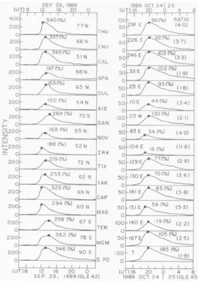
Since the second event is large, plots of hourly values for neu-tron monitors at high latitudes (>50◦latitude) for this event (GLE 42 of Sep. 29, 1989) are shown in Figure 9, left half. For com-parison, plots for the smaller event GLE 45 of Oct. 24, 1989 are shown in the right half of Figure 9. As can be seen, GLE 42 had a
maximum at 12-14 UT of Sept. 29, 1989 and lasted for 5-6 hours. The smaller event GLE 45 had a maximum at 19-20 UT of Oct. 24, 1989 and also lasted for 5-6 hours.
Figure 9 – Plots of hourly values of neutron monitor count rates at locations at high latitudes (>50◦, names and latitude-longitude indicated), for the event of Sep. 29, 1989 (left half) and Oct. 24, 1989 (right half). For Sep. 29, 1989, the GLE started at ∼11 UT and lasted for a few hours. For Oct. 24, 1989, the GLE started at ∼18 UT and lasted for a few hours. Numbers indicate magnitudes of the maximum increase in percentages.
Observations of relativistic solar protons during GLEs typi-cally begin with a rapid, anisotropic onset, with most particles moving anti-Sunward along the interplanetary magnetic field. Be-cause of pitch-angle scattering, which eventually leads to spatial diffusion, the distribution becomes more isotropic with time, and gradually decreases (or decays) as particles diffuse out of the in-ner heliosphere. GLE parameters during the initial phase of the event can be calculated for example, according to the method by Smart et al. (1971) and Debrunner & Lockwood (1980). For the evaluation of the asymptotic directions and the cutoff rigidi-ties for each NM location including effects of local time position and geomagnetic activity, the GEANT4 program MAGNETOCOS-MICS (http://reat.space.qinetiq.com/septimess/magcos/, contact Laurent Desorgher) can be used. Duldig (2001) has given
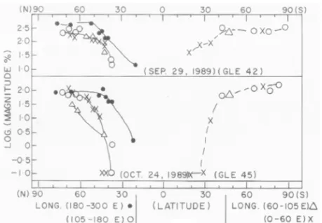
com-plete details of all these processes and of the methodology of how to allow for geomagnetic deflections and how to model the global GLE response. Some events present a more complicated picture, e.g., the GLE 44 of Oct. 22, 1989 (Ruffolo et al., 2005, discussed in Duldig, 2001 also, not considered here as the event was small, Climax increase only ∼10%) had a highly anisotropic spike at onset, while a second peak (hump) had bidirectional fluxes. The spike and hump may be explained in terms of a disturbed plasma region beyond Earth that scattered particles back. Inside the magnetosphere, deflection in geomagnetic field causes the effect to be seen at various longitudes simultaneously, though magnitudes may differ. Also, the UT hour of the event decides which longitudes (and therefore, which monitors) would see the largest magnitudes. However, the energy spectrum of different events may be different. Hence, the longitudinal patterns in diffe-rent events can be very diffediffe-rent from each other. In Figure 9, the percentage magnitudes for every location are indicated for both the events (GLE 42 in the left half, GLE 45 in the right half), and their ratios (magnitude of GLE 42/magnitude of GLE 45) are in-dicated in the right half of Figure 9. As can be seen, the ratios vary in a very wide range 2-12, indicating a considerable lack of similarity in their evolutions. Figure 10 shows the latitude dis-tributions of the magnitudes (ordinate, log scale), with different longitude belts shown by different symbols. In the top plot for GLE 42 (the strong event of Sep. 29, 1989), the mid-latitude northern American longitudes (full dots) seem to have larger mag-nitudes as compared to the other longitudes. In the bottom plot for GLE 45 (the weaker event of Oct. 24, 1989), there are three distinct groups of longitudinal distributions. Thus, considerable longitudinal anisotropies are indicated by differences in magni-tudes. Using information about geomagnetic deflections, the di-rection in space can be guessed as is done in the sophisticated analyses by many workers.
CONCLUSIONS AND DISCUSSION
The main purpose was to examine in a simple way (no sophistica-tions) the evolutions of the Ground Level Enhancements (GLEs) of Oct. 28, 2003 (the famous Halloween event) and the subse-quent Jan. 20, 2005 (a very large event in the declining phase of cycle 23). It was noticed that the Oct. 28, 2003 GLE was rather a small one (in contrast to the large CR Forbush decreases and geomagnetic Dst storms that occurred the next day, on Oct. 29, 2003). Hence, three more events were also studied, namely the largest GLE 5 of Feb. 23, 1956 (meager data), the second lar-gest GLE 42 of Sep. 29, 1989, and the fourth larlar-gest GLE 45 of
Figure 10 – Latitude distribution of the GLE magnitudes (ordinate, log scale) for GLE 42 of Sep. 29, 1989 in the top plot, and GLE 45 of Oct. 24, 1989 in the bottom plot. Different symbols indicate locations at different longitudes.
Oct. 24, 1989 (comparable to the third largest GLE 69 of Jan. 20, 2005). For each, the plots of few-minute and/or hourly values as also the latitude-longitude distributions of the GLE magnitu-des (percentage increases) were examined. It was noticed that at similar mid-latitudes, locations at different longitudes showed different latitude distributions, indicating that events had longi-tudinal anisotropies, more in some events, less in others. Thus, the present paper illustrates a simple way of detecting anisotro-pies in a qualitative way. Incidentally, in the present case, only the maximum enhancement magnitudes were used irrespective of the phases (maxima occurring at different UT times at different locations). If simultaneous magnitudes are used as these occur-red at specific UTs in succession, more details could be studied such as changes in the characteristics (spectra etc., or multiple populations) of the incoming particles, as is done in sophistica-ted analyses done by several workers. The present approach may be considered as a first look at a complex phenomenon.
From the satellite data of GOES-12 and GOES-11, it seems that the Forbush decrease of Oct. 29, 2003 was related to a CME emitted 5 days earlier, while the GLE of Oct. 28, 2003 was due to a prompt flare emission. Thus, these had different origins and hence their magnitudes could be unequal. During the last week of October 2003, so many solar features occurred that pinpoin-ting the origins of the GLE of Oct. 28, the FD of Oct. 29 and the mild CR decrease immediately before the Halloween event has become a confusing issue.
During the two GLE events of Oct. 28, 2003 and Jan. 20, 2005, the GOES X-ray prompt emission was of approximately the same power, but the GLE of Jan. 20, 2005 was much
lar-ger than the GLE of Oct. 28, 2003. The reason may probably be related to the different helio longitudes of the two flares with res-pect to the detection on the Earth. The pitch angle distribution and its temporal evolution may also be important. This needs a deeper study, beyond the limited scope and purpose (simplicity) of the present paper.
These conclusions from a simple examination are in general agreement with the conclusions obtained from detailed, sophisti-cated statistical analyses by several workers. Some details have been reported by other workers using 1-minute data. Thus, for the Oct. 28, 2003 event, Struminsky (2005a); Bieber et al. (2005a) found that for the Tsumeb neutron monitor (19◦S, 18◦E), a neu-tron injection was recorded at 11:04 UT which lasted for 9 minu-tes and the proton injection began at 11:11 UT and lasted over an hour. In our case, Tsumeb hourly values showed virtually no variation (Fig. 4 left half, 22ndplot). In some analyses, main data used were from satellites, and neutron monitor data were used only in a complementary way (e.g., Kuznetsov et al., 2005), nota-bly for spectral analysis (e.g., Mewaldt et al., 2005; Struminsky, 2005b). However, some analyses were done mainly from neutron monitor data in a rigorous way. Belov et al. (2005) analysed the Jan. 20, 2005 event and noted that the flux of relativistic pro-tons reached the Earth at ∼6:50 UT on Jan. 20, and at southern polar stations, the flux was about several thousands of percenta-ges. The characteristics of the cosmic ray energy spectrum, sotropy, differential and integral fluxes were obtained using ani-sotropic and compound models of solar cosmic ray variations. It was found that anisotropy contribution dominated during the first 15-20 minutes and quickly decreased along the time.
First particles came by a narrow beam from south-west direc-tion, and the flux along the IMF force line started to dominate only some time later. Similar studies for the two events (Oct. 28, 2003 and Jan. 20, 2005) are described by Vashenyuk et al. (2005 a,b,c), Moraal et al. (2005), Fl¨uckiger et al. (2005), S´aiz et al. (2005), Bieber et al. (2005 a,b), with some implication for ob-servation of solar neutrons also that seem to have arrived before the proton precipitation According to Vashenyuk et al. (2005a), relativistic solar cosmic rays responsible for the GLE of 20 Ja-nuary, 2005 were composed of two components, prompt and de-layed ones. The prompt component (PC) was very short-lived and extremely anisotropic. It had an exponential energetic spec-trum and caused the giant impulse-like increase effect at Antarc-tic NM stations South Pole and McMurdo. The arrival direction of PC was markedly different from the IMF direction. Possible cause of this effect could be scattering of narrow particle beam on the sharp kinks of IMF existing in front of the Earth during GLE onset. The delayed component had the power law energe-tic spectrum and wider pitch-angle distribution. It was respon-sible for increase effect at most NM stations of the worldwide network. The PC disappeared about 7.30 UT., after which, the delayed component dominated. Thus, a rigorous analysis reve-aled many finer details. Vashenyuk et al. (2005c) described a similar analysis of the Oct. 28, 2003 event and found two popu-lations clearly namely, prompt and delayed ones. The prompt so-lar protons caused an impulse-like increase at a few neutron mo-nitor stations looking perpendicular to the mean IMF direction. The delayed solar protons had slow intensity rise and arrived at Earth from the anti-sunward direction (looking along IMF). For the Jan. 20, 2005 event, Fl¨uckiger et al. (2005) mention that the initial pulse appeared to be a pencil beam of particles, although from the start of the event a bi-directional flux was also present. S´aiz et al. (2005) also found indication of two enhance-ments in particle flux at Earth, the second of which had a much lower anisotropy. A 2% increase was reported for a location in Tibet (30◦N, 91◦E), indicating a very hard spectrum (Miyasaka et al., 2005; Zhu et al., 2005). Some workers (private communi-cation) have mentioned to us that there are not two populations but a single population, arriving at the Earth with different pitch angles and the tail of the pitch angle distribution is 180◦ (anti-sunward direction). Obviously such fine details cannot be detec-ted by the simple method illustradetec-ted by us in the present paper.
Whereas the above analyses are highly sophisticated, they are very arduous and often seem to lead to ambiguous, uncertain re-sults, slightly different between different workers, probably due to the very nature of the methodology. It should be
remembe-red that GLEs are not a basic phenomena. They are distorted and filtered forms of the basic solar phenomena SEP (solar energe-tic parenerge-ticles) and depict only the comparatively high energy tail. Therefore, the information obtained about SEP from the GLE data is something like describing an elephant by examining its tail only. Substantial, reliable information about SEP characteristics can be obtained only from satellite data where effects of geomag-netic bending etc. do not exist. Even here, the SEPs emitted from the Sun may suffer some distortion during the transit and one has to guess how much the distortion could have been. With ground-based neutron monitors, things are much more complicated. Lot of effort is needed to find out the direction of arrival, but even if correctly estimated, this has hardly any relevance to the phy-sics of SEPs. The polar regions see the largest effects, but instru-ments in the polar region are very few, due to logistic difficulties. Bieber et al. (2002) mention a ‘Spaceship Earth’ network of po-lar neutron monitors, and in addition to the standard NM64 neutron monitor, the observing station at South Pole inclu-des a set of counters that are without the usual lead shielding. These “polar bare” detectors have a lower energy response than the NM64, which enables us to derive spectral information by comparing the relative response of the two types of detector to a solar particle event. One would have hoped that matters would im-prove with time in future, but Roger Pyle of Bartol Research Insti-tute said recently, “We regret to announce that the South Pole neu-tron monitor was closed on November 22, 2005, at the direction of NSF’s Office of Polar Programs”. A terrible loss indeed due to the availability of satellite data, the role of neutron monitors in the study of GLEs has been somewhat diluted, but hybrid study using the satellite data in conjunction with ground data may probably give a better insight. Nevertheless, the first observation of the gi-gantic event of Feb. 23, 1956 by neutron monitors half a century back, leaves a nostalgic memory of the unprecedented increase of several thousand percent, far larger than the sunspot cycle va-riations or Forbush decreases which hardly exceed fifty percent. The event not only aroused the curiosity of the scientific world, but gave a tremendous stimulation to cosmic ray research by ai-ding the large effort that followed during the IGY years 1957-1958.
ACKNOWLEDGEMENTS
Thanks are due to John W. Bieber and Roger Pyle of the Bartol Research Institute, University of Delaware for supplying priva-tely data of their neutron monitors, which are supported by NSF grant ATM-0527878. The present work was partially supported by FNDCT, Brazil under contract FINEP-537/CT.
REFERENCES
BELOV AV, BIEBER JW, EROSHENKO EA, EVENSON P, GVOZDEVSKY BB, PCHELKIN VV, PYLE R, VASHENYUK VE & YANKE VG. 2001. The “Bastille Day”; GLE 14 July, 2000 as observed by the worldwide neutron monitor network. Proc. 27thICRC, 3446–3449.
BELOV AV, EROSHENKO EA, MAVROMICHALAKI H, PLAINAKI C & YANKE VG. 2005. Ground level enhancement of the solar cosmic rays on January 20, 2005. Proc. 29thInt. Cosmic Ray Conference, 2005, Pune, India, 1: 189–192.
BIEBER JW, DR¨OGE W, EVENSON PA, PYLE R, RUFFOLO D, PINSOOK U, TOOPRAKAI P, RUJIWARODOM M, KHUMLUMLERT T & KRUCKER S. 2002. Energetic Particle Observations during the 2000 July 14 Solar Event. Astrophys. J., 567: 622–634.
BIEBER JW, CLEM J, EVENSON P, PYLE R, BLAKE JB, MULLIGAN T, RUFFOLO D & S´AIZ A. 2005a. Observation of Neutron and Gamma Ray Emission from the October 28, 2003 Solar Flare. Proc. 29thInt. Cosmic Ray Conference, 2005, Pune, India, 1: 57–58.
BIEBER JW, CLEM J, EVENSON P, PYLE R, DULDIG M, HUMBLE J, RUFFOLO D, RUJIWARODOM M & S´AIZ A. 2005b. Largest GLE in Half a Century: Neutron Monitor Observations of the January 20, 2005 Event. Proc. 29thInt. Cosmic Ray Conference, 2005, Pune, India, 1: 237–240. CLEM JM & DORMAN LI. 2000. Neutron monitor response functions. Space Sci. Rev., 93: 335–359.
COHEN CMS, STONE EC, MEWALDT RA, LESKE RA, CUMMINGS AC, MASON GM, DESAI MI, VON ROSENVINGE TT & WIEDENBECK ME. 2005. Heavy ion abundances and spectra from the large solar energe-tic parenerge-ticle events of October-November 2003. J. Geophys. Res., 110: A09S16, doi:10.1029/2005JA011004.
DEBRUNNER H & LOCKWOOD JA. 1980. The spatial anisotropy, rigidity spectrum, and propagation characteristics of the relativistic solar parti-cles during the event on May 7, 1978. J. Geophys. Res., 85(A11): 6853– 6860.
DUGGAL SP. 1979. Relativistic Solar Cosmic Rays. Rev. Geophys. Space Phys. 17: 1021–1058.
DULDIG ML. 2001. Australian cosmic ray modulation research. Publ. Astron. Soc. Australia, 18(1): 12–40.
FEDOROV YU, STEHLIK M, KUDELA K & KASSOVICOVA J. 2002. Non-diffusive particle pulse transport – Application to an anisotropic solar GLE. Solar Phys., 208(2): 325–334.
FL¨UCKIGER EO, BUTIKOFER R, MOSER MR & DESORGHER L. 2005. The Cosmic Ray Ground Level Enhancement during the Forbush Decre-ase in January 2005. Proc. 29thInt. Cosmic Ray Conference, 2005, Pune, India, 1: 225–228.
FORBUSH SE. 1946. Three unusual cosmic-ray increases possibly due to charged particles from the Sun. Phys. Rev., 70: 771–772.
GOPALSWAMY N, XIE H, YASHIRO S & USOKIN I. 2005. Coronal mass ejections and ground level enhancements. Proc. 29thInt. Cosmic Ray Conference, 2005, Pune, India, 1: 169–172.
KAHLER SW, CLIVER EW, CANE HV, McGUIRE RE, STONE RG & SHEELEY JR NR. 1986. Solar filament eruptions and energetic particle events. Astrophys. J., 302: 504–510.
KANE RP & AHLUWALIA HS. 1957. Solar flare effect on cosmic ray meson intensity at Gulmarg. Current Science, 26: 83–84.
KUZNETSOV SN, KURT VG, YUSHKOV BYU, MYAGKOVA IN, KUDELA K, KASSOVICOVA J & SLIVKA M. 2005. Proton acceleration during 20 January 2005 solar flare: CORONAS-F observations of high-energy gamma emission and GLE. Proc. 29thInt. Cosmic Ray Conference, 2005, Pune, India, 1: 49–52.
LABRADOR AW, LESKE RA, MEWALDT RA, STONE EC & VON ROSEN-VINGE TT. 2005. High Energy Ionic Charge State Composition in the October/November 2003 and January 20, 2005 SEP Events. Proc. 29th Int. Cosmic Ray Conference, 2005, Pune, India, 1: 99–102.
LOVELL JL, DULDIG ML & HUMBLE JE. 1998. An extended analysis of the September 1989 cosmic ray ground level enhancement. J. Geophys. Res., 103: 23733–23742.
MEWALDT RA, LOOPER MD, COHEN CMS, MASON GM, HAGGERTY DK, DESAI MI, LABRADOR AW, LESKE RA & MAZUR JE. 2005. Solar-particle energy spectra during the large events of October-November 2003 and January 2005. Proc. 29thInt. Cosmic Ray Conference, 2005, Pune, India, 1: 111–114.
MEYER P, PARKER EN & SIMPSON JA. 1956. Solar Cosmic Rays of February, 1956 and their Propagation through Interplanetary Space. Phys. Rev., 104: 768–783.
MIROSHNICHENKO LI, DE KONING CA & PEREZ-ENRIQUEZ R. 2000. Large solar event of September 29, 1989: ten years after. Space Sci. Rev., 91: 615–675.
MIROSHNICHENKO LI, KLEIN KL, TROTTET G, LANTOS P, VASHENYUK EV, BALABIN YV & GVOZDEVSKY BB. 2005. Relativistic nucleon and electron production in the 2003 October 28 solar event. J. Geophys. Res., 110: A09S08, doi:10.1029/2004JA010936.
MIYASAKA H, TAKAHASHI E, SHIMODA S, YAMADA Y, KONDO I, TSUCHIYA H, MAKISHIMA K, ZHU FR, TAN YH, HU HB, TANG YQ, CLEM J & YBJ NM COLLABORATION. 2005. The Solar Event on 20 January 2005 observed with the Tibet YBJ Neutron monitor observatory. Proc. 29thInt. Cosmic Ray Conference, 2005, Pune, India, 1: 241–244. MORAAL H, McCRACKEN KG, SCHOEMAN CC & STOKER PH. 2005. The Ground Level Enhancements of 20 January 2005 and 28 October 2003. Proc. 29thInt. Cosmic Ray Conference, 2005, Pune, India, 1: 221–224.
RAO UR. 1976. High energy cosmic ray observations during August 1972. Space Sci. Rev., 19: 533–577.
REEVES GD, CAYTON TE, GARY SP & BELIAN RD. 1992. The great solar energetic particle events of 1989 observed from geosynchronous orbit. J. Geophys. Res., 97: 6219–6226.
RUFFOLO D, TOOPRAKAI P, RUJIWARODOM M, KHUMLUMLERT T, WECHAKAMA M, BIEBER JW, EVENSON P & PYLE R. 2005. Relati-vistic Solar Protons on 1989 October 22: Injection and Transport along Both Legs of a Closed Interplanetary Magnetic Loop. Proc. 29th Int. Cosmic Ray Conference, 2005, Pune, India, 1: 307–310.
RYAN JM, LOCKWOOD JA & DEBRUNNER H. 2000. Solar energetic particles. Space Sci. Rev., 93: 35–53.
S´AIZ A, RUFFOLO D, RUJIWARODOM M, BIEBER JW, CLEM J, EVEN-SON P, PYLE R, DULDIG ML & HUMBLE JE. 2005. Relativistic Parti-cle Injection and Interplanetary Transport during the January 20, 2005 ground level enhancement. Proc. 29thInt. Cosmic Ray Conference, 2005, Pune, India, 1: 229–232.
SARABHAI V, DUGGAL SP, RAZDAN HL & SASTRY TSG. 1956. A Solar Flare Type Increase in Cosmic Rays at Low Latitude. Proc. Ind. Acad. Sci., 43: 309–318.
SHEA MA & SMART DF. 1990. A summary of major proton events. Solar Phys., 127: 297–320.
SHEA MA & SMART DF. 1996. Unusual intensity-time profiles of ground-level solar proton events. AIP Conference Proceedings, 374(1): 131–139.
SHEA MA & SMART DF. 2001a. Solar proton and GLE event frequency: 1955-2000. Proc. 27thICRC, 3401–3404.
SHEA MA & SMART DF. 2001b. Vertical cutoff rigidities for cosmic ray stations since 1955. Proc. 27thICRC, 4063–4064.
SIMNETT GM. 2006. Timing of the relativistic proton acceleration res-ponsible for the GLE on 20 January, 2005, Astron. Astrophys., 445: 715–724.
SMART DF & SHEA MA. 1989. Solar proton events during the past three solar cycles. J. Spacecraft, 26: 403–415.
SMART DF, SHEA MA & TANSKANEN PJ. 1971. A Determination of the Spectra, Spatial Anisotropy, and Propagation Characteristics of the Rela-tivistic Solar Cosmic-Ray Flux on November 18, 1968. 12thInternational Conference on Cosmic Rays, Hobart, Conference Papers (University of Tasmania), 2: 483–488.
STRUMINSKY AB. 2005a. On Possibility of Prolonged Two Step Produc-tion of High Energy Neutrons during the Solar Flare on 28 October 2003. Proc. 29thInt. Cosmic Ray Conference, 2005, Pune, India, 1: 45–48. STRUMINSKY AB. 2005b. Variations of solar proton spectrum during the ground level enhancement of 2005 January 20. Proc. 29thInt. Cosmic Ray Conference, 2005, Pune, India, 1: 201–204.
TIMOFEEV VE, KRIVOSHAPKIN PA, GRIGORYEV VG, PRIHODKO AN, MIGUNOV VM & FILIPPOV AT. 2005. Increase of the Solar Energetic Particle Flux on January 20, 2005. Proc. 29thInt. Cosmic Ray Confe-rence, 2005, Pune, India, 1: 205–208.
TSYGANENKO NA. 1989. A magnetospheric magnetic field model with a warped tail current sheet. Planet. Space Sci., 37: 5–20.
VASHENYUK EV, BALABIN YU V, GVOZDEVSKY BB, KARPOV SN, YANKE VG, EROSHENKO EA, BELOV AV & GUSHCHINA RT. 2005a. Rela-tivistic solar cosmic rays in January 20, 2005 event on the ground based observations. Proc. 29thInt. Cosmic Ray Conference, 2005, Pune, India, 1: 209–212.
VASHENYUK EV, BALABIN YU V, BAZILEVSKAYA GA, MAKHMUTOV VS, STOZHKOV YU I & SVIRZHEVSKY NS. 2005b. Solar Particle Event 20 January, 2005 on stratosphere and ground level observations. Proc. 29thInt. Cosmic Ray Conference, 2005, Pune, India, 1: 213–216. VASHENYUK EV, BALABIN YU V, GVOZDEVSKY BB, MIROSHNICHENKO LI, KLEIN KL, TROTTET G & LANTOS P. 2005c. Energetic solar particle dynamics during 28 October, 2003 GLE. 29thInt. Cosmic Ray Confe-rence, 2005, Pune, India, SH Abstracts page 54.
ZHU FR, TANG YQ, ZHANG Y, LU H, ZHANG JL & TAN YH. 2005. A pos-sible GLE event in association with solar flare on January 20, 2005. Proc. 29thInt. Cosmic Ray Conference, 2005, Pune, India, 1: 217–220.
NOTE ABOUT THE AUTHOR
Rajaram Purushottam Kane. Born on 12 November 1926 at Damoh, MP, India. M.Sc. Physics in 1946 from Banaras Hindu University, India. Ph.D. in 1953 from Bombay University, India. Visited the Institute of Nuclear Studies at the University of Chicago, USA as a Fulbright Smith-Mundt post-doc fellow during 1953-1954. From 1955 to 1978, worked as a research fellow and Professor at PRL (Physical Research Laboratory), Ahmedabad, India. Participated actively (Coordinator of Cosmic Ray data in India) in the activities of IGY (International Geophysical Years, 1957-1958). Since 1978, working as a Researcher at INPE (Instituto Nacional de Pesquisas Espaciais), S˜ao Jos´e dos Campos, SP, Brazil.