www.geosci-model-dev.net/4/543/2011/ doi:10.5194/gmd-4-543-2011
© Author(s) 2011. CC Attribution 3.0 License.
Geoscientific
Model Development
The HadGEM2-ES implementation of CMIP5 centennial
simulations
C. D. Jones1, J. K. Hughes1, N. Bellouin1, S. C. Hardiman1, G. S. Jones1, J. Knight1, S. Liddicoat1, F. M. O’Connor1, R. J. Andres2, C. Bell3,†, K.-O. Boo4, A. Bozzo5, N. Butchart1, P. Cadule6, K. D. Corbin7,*, M. Doutriaux-Boucher1, P. Friedlingstein8, J. Gornall1, L. Gray9, P. R. Halloran1, G. Hurtt10,16, W. J. Ingram1,11, J.-F. Lamarque12,
R. M. Law7, M. Meinshausen13, S. Osprey9, E. J. Palin1, L. Parsons Chini10, T. Raddatz14, M. G. Sanderson1, A. A. Sellar1, A. Schurer5, P. Valdes15, N. Wood1, S. Woodward1, M. Yoshioka15, and M. Zerroukat1
1Met Office Hadley Centre, Exeter, EX1 3PB, UK
2Environmental Sciences Division, Oak Ridge National Laboratory, Oak Ridge, TN 37831-6335, USA 3Meteorology Dept, University of Reading, Reading, RG6 6BB, UK
4National Institute of Meteorological Research, Korea Meteorological Administration, Korea 5School of GeoSciences, University of Edinburgh, The King’s Buildings, Edinburgh EH9 3JW, UK 6Institut Pierre-Simon Laplace, Universit´e Pierre et Marie Curie Paris VI, 4 Place de Jussieu, case 101,
75252 cedex 05 Paris, France
7Centre for Australian Weather and Climate Research, CSIRO Marine and Atmospheric Research, Aspendale,
Victoria, Australia
8College of Engineering, Mathematics and Physical Sciences, University of Exeter, Exeter, EX4 4QF, UK 9National Centre for Atmospheric Science, Department of Physics, University of Oxford, Oxford, OX1 3PU, UK 10Department of Geography, University of Maryland, College Park, MD 21403, USA
11Department of Physics, University of Oxford, Oxford, OX1 3PU, UK 12Atmospheric Chemistry Division, UCAR, Boulder, USA
13Earth System Analysis, Potsdam Institute for Climate Impact Research, Germany 14Max Planck Institute for Meteorology, Hamburg, Germany
15School of Geographical Sciences, University of Bristol, Bristol BS81SS, UK
16Pacific Northwest National Laboratory, Joint Global Change Research Institute, University of Maryland, College Park,
MD 20740, USA
*now at: Colorado State University, Fort Collins, USA †deceased, 20 June 2010
Received: 7 March 2011 – Published in Geosci. Model Dev. Discuss.: 31 March 2011 Revised: 14 June 2011 – Accepted: 19 June 2011 – Published: 1 July 2011
Abstract. The scientific understanding of the Earth’s mate system, including the central question of how the cli-mate system is likely to respond to human-induced pertur-bations, is comprehensively captured in GCMs and Earth System Models (ESM). Diagnosing the simulated climate re-sponse, and comparing responses across different models, is crucially dependent on transparent assumptions of how the GCM/ESM has been driven – especially because the im-plementation can involve subjective decisions and may dif-fer between modelling groups performing the same experi-ment. This paper outlines the climate forcings and setup of
Correspondence to:C. D. Jones ([email protected])
1 Introduction
Phase 5 of the Coupled Model Intercomparison Project (CMIP5) is a standard experimental protocol for studying the output of coupled ocean-atmosphere general circulation models (GCMs). It provides a community-based infrastructure in support of climate model diagnosis, val-idation, intercomparison, documentation and data access. The purpose of these experiments is to address outstanding scientific questions that arose as part of the IPCC Fourth Assessment report (AR4) process, improve understanding of climate, and to provide estimates of future climate change that will be useful to those considering its possible consequences and the effect of mitigation strategies.
CMIP5 began in 2009 and is meant to provide a frame-work for coordinated climate change experiments over a five year period and includes simulations for assessment in the IPCC Fifth Assessment Report (AR5) as well as others that extend beyond the AR5. The IPCC’s AR5 is scheduled to be published in September 2013. CMIP5 promotes a standard set of model simulations in order to:
– evaluate how realistic the models are in simulating the recent past,
– provide projections of future climate change on two time scales, near term (out to about 2035) and long term (out to 2100 and beyond), and
– understand some of the factors responsible for differ-ences in model projections, including quantifying some key feedbacks such as those involving clouds and the carbon cycle.
A much more detailed description can be found on the CMIP5 project webpages (see URL 1 in Appendix A) and in Taylor et al. (2009).
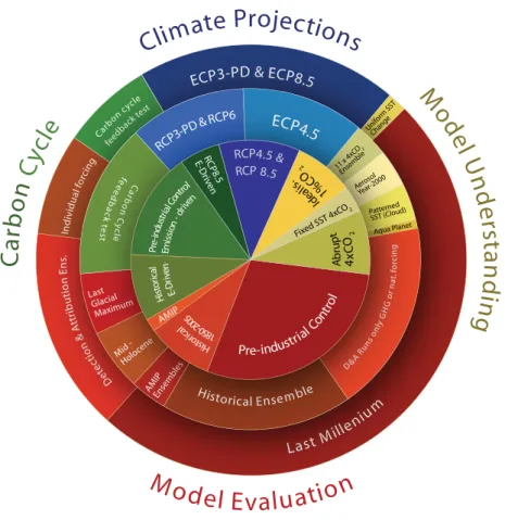
There are a number of new types of experiments proposed for CMIP5 in comparison with previous incarnations. As in previous intercomparison exercises, the main focus and effort rests on the longer time-scale (“centennial”) experiments, including now emission-driven runs of models that include a coupled carbon-cycle (ESMs). These centennial experi-ments are being performed at the Met Office Hadley Centre with the HadGEM2-ES Earth System model (Collins et al., 2011; Martin et al., 2011); a configuration of the Met Of-fice’s Unified Model. Figure 1 outlines the main experiments and groups them into categories. The inner circle denotes “core” priority experiments with tier 1 (middle circle) and tier 2 (outer circle) having successively lower priority. Ex-periments are split between climate projections (blue), ide-alised experiments aimed at elucidating process understand-ing in the models (yellow), model evaluation, includunderstand-ing pre-industrial control runs and historical experiments (red), and additional experiments for models with a coupled carbon cy-cle (green).
In the following, we briefly describe HadGEM2-ES ESM, which is documented in detail in Collins et al. (2011). HadGEM2-ES is a coupled AOGCM with atmospheric reso-lution of N96 (1.875◦×1.25◦)with 38 vertical levels and an ocean resolution of 1◦(increasing to 1/3◦at the equator) and 40 vertical levels. HadGEM2-ES also represents interactive land and ocean carbon cycles and dynamic vegetation with an option to prescribe either atmospheric CO2concentrations or
to prescribe anthropogenic CO2emissions and simulate CO2
concentrations as described in Sect. 2. An interactive tropo-spheric chemistry scheme is also included, which simulates the evolution of atmospheric composition and interactions with atmospheric aerosols. The model timestep is 30 min (atmosphere and land) and 1 h (ocean). Extensive diagnos-tic output is being made available to the CMIP5 multi-model archive. Output is available either at certain prescribed fre-quencies or as time-average values over certain periods as detailed in the CMIP5 output guidelines (see URL 2 in Ap-pendix A).
The CMIP5 simulations include 4 future scenarios re-ferred to as “Representative Concentration Pathways” or RCPs (Moss et al., 2010). These future scenarios have been generated by four integrated assessment models (IAMs) and selected from over 300 published scenarios of future greenhouse gas emissions resulting from socio-economic and energy-system modelling. These RCPs are labelled ac-cording to the approximate global radiative forcing level in 2100 for RCP8.5 (Riahi et al., 2007), during stabilisation af-ter 2150 for RCP4.5 (Clarke et al., 2007; Smith and Wigley, 2006) and RCP6 (Fujino et al., 2006) or the point of maxi-mal forcing levels in the case RCP3-PD (van Vuuren et al., 2006, 2007), with PD standing for “Peak and Decline”. The latter scenario has previously been known as RCP2.6, as ra-diative forcing levels decline towards 2.6 Wm−2 by 2100. Note that these radiative forcing levels are illustrative only, because greenhouse gas concentrations, aerosol and tropo-spheric ozone precursors are prescribed, resulting in a wide spread in radiative forcings across different models.
The experimental protocol involves performing a histori-cal simulation (defined for HadGEM2-ES as 1860 to 2005) using the historical record of climate forcing factors such as greenhouse gases, aerosols and natural forcings such as solar and volcanic changes. The model state at 2005 is then used as the initial condition for the 4 future RCP simulations. Fur-ther extension of the RCP simulations to 2300 is also imple-mented as detailed in the RCP White Paper (see URL 3 in Appendix A) and Meinshausen et al. (2011).
Many of these experiments require technical implementa-tion by means of either or both of the following:
Unif orm SST feed back test Car bon cycle D et ec ti o n & A tt ri b u ti o n E n s. Ind ivid ua
l fo
rcin
g
Last M i
lleni
u m
ECP3-PD & ECP8.5
RCP3
-PD & RC
P6
ECP4.5
D&
A R un
s o
nly G HG or na t. f orc in g fe e e d b a c k t e st C a rb o n C y c le AMIP Ensembles
Mid -Holoc
ene
Last Glacial
Maximum
Historical Ensemble RCP4.5 & RCP8.5 E-Driv en 1% CO 2 4x C O2 Id ea lis . A b ru p t
Pre-industrial
Con tro l E-D ri ve n Em issi
on -
drive n AMIP Pr e-indu stria
l Con trol
Fixed SST 4xC O2 His tor ica l H is to ri ca l 1 85 0-2 00 5 RCP 8.5
M odel Evaluation
C
a
rb
o
n
C
yc
le
Clim
ate Projections
M
o
d
el
U
n
d
e
rs
ta
n
d
in
g
Fig. 1. Schematic of CMIP5 centennial simulations, adapted from Taylor et al. (2009) with each experiment being represented by an area that is proportional to the experiment’s length in model years. The inner circle denotes “core” priority experiments with tier 1 (middle circle) and tier 2 (outer circle) having successively lower priority. Experiments are split between climate projections (blue), idealised experiments aimed at elucidating process understanding in the models (yellow), model evaluation, including pre-industrial control runs and historical experiments (red), and additional experiments for models with a coupled carbon cycle (green). See CMIP5 project webpage (Appendix A) for more detailed information. (D&A: detection and attribution, ECP: extended RCP simulations to 2300).
– code changes to alter the scientific behaviour of the model, such as to decouple various feedbacks and in-teractions (e.g. the “uncoupled” carbon cycle experi-ments).
This paper presents in detail the technical aspects of how these model forcings are implemented in HadGEM2-ES. It is not our intention here to present scientific results from the experiments. This analysis will be left for subsequent work.
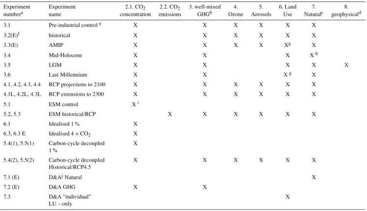
The CMIP5 experiments performed with HadGEM2-ES are listed in Table 1 along with the relevant forcings for each experiment. How these forcings are then implemented is detailed in the following sections with Sect. 2 describing the atmospheric CO2 concentrations for the
concentration-driven runs as well as the CO2emission assumptions for the
emission-driven experiments. Section 3 details the boundary conditions of atmospheric concentrations of the other well-mixed greenhouse gases. Tropospheric and stratospheric ozone assumptions are detailed in Sect. 4. Section 5 de-tails the treatment of aerosols, while Sect. 6 documents that
applied to land use pattern changes. Natural forcings, both solar and volcanic, are described in Sect. 7. Apart from these recent history, centennial 21st century and longer-term ex-periments, we describe as well the setup for the palaeocli-matic runs in Sect. 8. The more general issue of how the en-semble members are branched off the control run is described in Sect. 9, and Sect. 10 concludes. A list of URL locators for websites holding relevant data is included as an Appendix.
2 Carbon dioxide 2.1 CO2concentration
For simulations requiring prescribed atmospheric CO2
con-centrations, a single global 3-D constant provided as an an-nual mean mass mixing ratio was used – linearly interpolated in the model at each timestep. This prescribed CO2
Table 1. Overview of CMIP5 experiments and their prescribed boundary conditions, i.e., atmospheric concentrations or emissions. This Table lists the climate forcings required to be changed from the control run (Experiment 3.1) in order to set-up and perform each CMIP5 experiment. The presence of a cross denotes that that forcing is changed, and is documented in the section listed in the column title. An absence of a cross does not mean that forcing is missing, but that it is kept the same as in the control run.
Experiment Experiment 2.1. CO2 2.2. CO2 3. well-mixed 4. 5. 6. Land 7. 8.
numbera name concentration emissions GHGb Ozone Aerosols Use Naturalc geophysicald
3.1 Pre-industrial controle X X X X X X
3.2(E)f historical X X X X X X
3.3(E) AMIP X X X X Xg X
3.4 Mid-Holocene X X X Xh
3.5 LGM X X X X X
3.6 Last Millennium X X Xg X
4.1, 4.2, 4.3, 4.4 RCP projections to 2100 X X X X X X
4.1L, 4.2L, 4.3L RCP extensions to 2300 X X X X X X
5.1 ESM control Xi
5.2, 5.3 ESM historical/RCP X X X X X X
6.1 Idealised 1 % X
6.3, 6.3 E Idealised 4×CO2 X
5.4(1), 5.5(1) Carbon-cycle decoupled 1 %
X
5.4(2), 5.5(2) Carbon-cycle decoupled Historical/RCP4.5
X X X X X X
7.1 (E) D&AjNatural X
7.2 (E) D&A GHG X X
7.3 D&A “individual” LU – only
X
aexperiments are numbered as per Centennial experiments (Table B in Taylor et al., 2009). We explicitly don’t consider the idealised SST experiments 6.2, 6.4, 6.5, 6.6, 6.7, 6.8 which will be documented elsewhere.b“well mixed GHG” here covers CH4, N2O, and halocarbons, but not CO2which is treated in Sect. 2. “Ozone” covers tropospheric and stratospheric and includes emissions of pre-cursor gases which affect tropospheric ozone (see Sect. 4)c“natural” forcing covers both solar and volcanic changes (Sect. 7)d “geophysical” here is taken to include changes in: prescribed ice sheet extent (incl. height), land-sea mask, ocean bathymetry.ethe control run does have “forcing” in that we prescribe several things to be constant. The relevant sections describe how each climate forcing is set up for the control run. The Table then lists aspects which differ from the control (either by being time varying in scenarios, or by being held constant at different values such as in the 4×CO2simulation).f“(E)” denotes that an initial-condition ensemble is required for these experiments. Section 9 describes how the initial conditions are derived.gland-use in the AMIP and last millennium experiments is described in their respective Sects. (9.2, 8.3) rather than the land-use Sect. 6.hpalaeoclimate orbital forcing is described in Sect. 8 rather than under solar forcing in Sect. 7.1.iThe “ESM control” simulation actually has an absence of forcing as CO2is simulated in this experiment, not prescribed.j“D&A” stands for detection and attribution.
carbon cycle. The oceanic partial pressure of CO2,pCO2, is
always simulated prognostically from this, i.e. it is not itself prescribed.
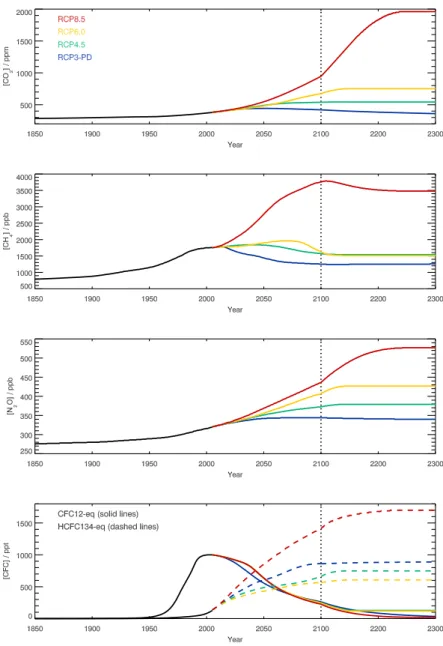
The CO2concentrations used were taken from the CMIP5
dataset (see URL 4 in Appendix A). The historical part of the concentrations (1860–2005) is derived from a combi-nation of the Law Dome ice core (Etheridge et al., 1996), NOAA global mean data (see URL 5 in Appendix A) and measurements from Mauna Loa (Keeling et al., 2009). Af-ter 2005, CO2concentrations recommended for CMIP5 were
calculated for the 21st century from harmonized CO2
emis-sions of the four IAMs that underlie the four RCPs. Be-yond 2100, these concentrations were extended, so that the CO2 concentrations under the highest RCP, RCP8.5,
sta-bilize just below 2000 ppm by 2250. Both the medium RCPs smoothly stabilize around 2150, with RCP4.5 stabi-lizing close to the 2100 value of the former SRES B1 sce-nario (∼540 ppm). The lower RCP, RCP3-PD, illustrates a
world with net negative emissions after 2070 and sees de-clining CO2 concentrations after 2050, with a decline of
0.5 ppm yr−1around 2100 (see Fig. 2). These CO2
concen-trations are prescribed in HadGEM2-ES’s historical, AMIP, RCP simulations and the carbon-cycle uncoupled experi-ments. The detection and attribution experiments with time varying CO2also use these values, but the detection and
at-tribution experiments with fixed CO2levels use a constant,
pre-industrial value of 286.3 ppm. This CMIP5 dataset also provides the CO2 concentration used for the pre-industrial
control simulation (taken here to be 1860 AD), which is 286.3 ppm. CO2 for the palaeoclimate simulations is
de-scribed in Sect. 8. More details on the CMIP5 CO2
con-centrations and how they were derived are provided in Mein-shausen et al. (2011).
Fig. 2.Well mixed GHG concentrations used for concentration driven simulations:(a)CO2,(b)CH4,(c)N2O,(d)halocarbons. Plotted are
historical observed concentrations (black lines), and the four RCPs as well as their extensions beyond 2100 (RCP8.5: red; RCP6: yellow; RCP4.5: green; RCP3-PD: blue). See Meinshausen et al. (2011) for further details. Note that the x-axis beyond 2100 is compressed.
sensitivity and the climate-carbon cycle feedback. For the idealised annual 1 % increase in CO2 concentration, we
start from the control-run level of 286.3 ppm in 1859 up to 4×CO2(1144 ppm) after 140 yr (Experiment 6.1).
Equiva-lently, our instantaneous quadrupling to 4×CO2uses a
con-centration of 1144 ppm in order to allow diagnosis of short-term forcing adjustments and equilibrium climate sensitivi-ties (Experiment 6.3).
2.1.1 Decoupled carbon cycle experiments
Using additional code modifications to the appropriate mod-ules of the HadGEM2-ES model, it is possible to decouple
different carbon-cycle feedbacks. For the decoupled carbon cycle experiments (5.4, 5.5) we decoupled the climate and carbon cycle in 2 different ways. The C4MIP intercompar-ison exercise (Friedlingstein et al., 2006) defined an “UN-COUPLED” methodology in which only the carbon cycle component responded to changes in atmospheric CO2
lev-els. Gregory et al. (2009) additionally describe the coun-terpart experiment where only the model’s radiation scheme responds to changes in CO2. Gregory et al. (2009)
Hence we performed the biogeochemically coupled (“BGC”) experiments (5.4) in which the models biogeo-chemistry is coupled (i.e., the biogeobiogeo-chemistry modules re-spond to the changing atmospheric CO2 concentration) and
the radiation scheme is uncoupled (and uses the preindustrial level of CO2which is held constant) and also radiatively
cou-pled (“RAD”) experiments (5.5) in which the model’s radia-tion scheme is allowed to respond to changes in atmospheric CO2levels, but the biogeochemistry components (land
veg-etation and ocean chemistry and ecosystem) use a constant CO2level, again set to the preindustrial value. Both
decou-pled experiments can be achieved with single simulations in which time-varying or time-fixed values of CO2are used as
input data to the respective sections of model code. We per-formed both BGC and RAD experiments for the idealised (1 %) and transient, multi-forcing (historical/RCP4.5) sce-narios.
2.2 CO2emissions
2.2.1 Emissions data
In addition to running with prescribed atmospheric CO2
con-centrations, HadGEM2-ES can be configured to run with a fully interactive carbon cycle. Here, atmospheric CO2
is treated as a 3-D prognostic tracer, transported by atmo-spheric circulation, and free to evolve in response to pre-scribed surface emissions and simulated natural fluxes to and from the oceans and land. This approach is required for the “Emission-driven” simulations (5.1–5.3) shown in green in Fig. 1, and it also allows additional model evaluation by comparison with flask and station measuring sites such as at Mauna Loa (e.g. Law et al., 2006; Cadule et al., 2010).
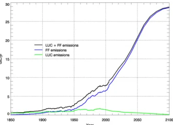
A 2-D timeseries of total anthropogenic emissions was constructed by summing contributions from fossil fuel use and land-use change. For the historical simulation, annual mean emissions from fossil fuel burning, cement manufac-ture, and gas-flaring were provided on a 1◦×1◦ grid from 1850 to 1949 (Boden et al., 2010), with monthly means from 1950 to 2005 (Andres et al., 2011). For the RCP8.5 simula-tion, the harmonized fossil fuel emissions for 2005 to 2100 were used (as available in the RCP database, see URL 6 in Appendix A). The land use change (LUC) emissions are based on the regional totals of Houghton (2008), which were provided as annual means of the period 1850–2005. Within each of the ten regions the emissions were linearly weighted by population density on a 1◦×1◦grid (for more
informa-tion, see URL 7 in Appendix A). These population data were also used by Klein Goldewijk (2001) and are linearly interpo-lated between the years 1850, 1900, 1910, 1920, 1930, 1940, 1950, 1960, 1970, 1980, and 1990. After the year 1990 popu-lation density is assumed to stay constant. Additionally, high population density was set to a limit of 20 persons per km2to avoid large emissions in urban centres. The weighting with population data inhibits land use change emissions in deserts
and high northern latitudes, which improves the latitudinal distribution of the emissions. However, the method is insuf-ficient to provide realistic local land use change emissions (e.g. in tropical forests).
The gridded (1◦×1◦) fossil fuel and land-use emissions data, originally provided as a flux per gridbox, were con-verted to flux per unit area, then regridded as annual means onto the HadGEM2-ES model grid. A small scaling adjust-ment was made after regridding to ensure the global totals matched those of the 1◦×1◦data exactly. Future emissions were not provided with spatial information so we scaled the 2005 geographical pattern for fossil-fuel and land-use emis-sions to give the correct global total into the future. The CO2 emissions are updated daily in the model by linearly
interpolation between the annual values (or monthly, from 1950–2005). HadGEM2-ES has the functionality to inter-actively simulate land-use emissions of CO2directly from a
prescribed scenario of land-use change and simulated vegeta-tion cover and biomass (see Sect. 6). However, the model has not been fully evaluated in this respect, so for CMIP5 exper-iments we disable this feature and choose rather to prescribe reconstructed land-use emissions from Houghton (2008). By simulating changes in carbon storage due to imposed land use change, but imposing land-use CO2emissions to the
at-mosphere from an external dataset we introduce some degree of inconsistency in this simulation. Work is required to eval-uate and improve the simulation of land-use emissions so that they can be used interactively in such simulations in the fu-ture.
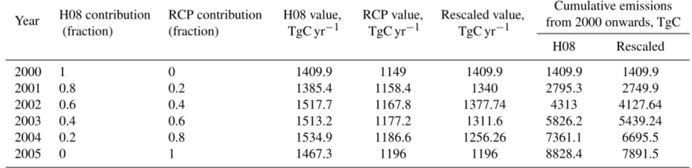
The uncertainty in annual land-use emissions of±0.5 GtC (cf. Le Qu´er´e et al., 2009) is relatively large compared to the total land use emissions (an estimated 1.467 GtC in 2005, Houghton, 2008). The RCP scenarios have been harmonised towards the average LUC emission value of all four original IAM emission estimates, i.e., 1.196 GtC in 2005. This is substantially lower than the value calcu-lated by Houghton (2008) of 1.467 GtC in the same year, although still within the uncertainty. The climate-carbon cycle modelling community preferred to use the original Houghton (2008) estimates for historical emissions. A smooth transition between the historical and the RCP simula-tions was ensured by scaling the last five years of the histori-cal LUC emissions to factor in a linearly-increasing contribu-tion from the harmonised RCP values. In 2001 the two val-ues were combined in the ratio 80 %:20 % (Houghton: RCP), followed by 60 %:40 % in 2002, and so on until 0 %:100 % (i.e. the RCP value) in 2005, as shown in Fig. 3.
Fig. 3. Global land use emissions data during the transition from the historical simulation to the RCP 8.5 simulation. The Houghton (2008) land use emissions data (black line) were scaled to meet the RCP data (blue line), resulting in the red line with trian-gles, which replaced the black line during 2000–2005.
2.2.2 Carbon conservation
In the emissions-driven experiments, conservation of carbon in the earth system is required. The concentration of atmo-spheric CO2influences the carbon exchange with the oceans
and terrestrial biosphere. Any drift in atmospheric CO2will
modify these fluxes accordingly, and thereby impact the land and ocean carbon stores as well as the climate itself. While the transport of atmospheric tracers in HadGEM2-ES is de-signed to be conservative, the conservation is not perfect and in centennial scale simulations this non-conservation be-comes significant. This has been addressed by employing an explicit “mass fixer” which calculates a global scaling of CO2to ensure that the change in the global mean mass
mix-ing ratio of CO2in the atmosphere matches the total flux of
CO2into or out of it each timestep (Corbin and Law, 2011).
Figure 5 demonstrates HadGEM2-ES’s ability to conserve atmospheric CO2, following implementation of the mass
fixer scheme described here. The evolution of the atmo-spheric CO2burden calculated by the model matches almost
exactly the accumulation over time of the CO2flux to the
at-mosphere. The lower panel of Fig. 5 shows the difference between the two. This residual difference is most likely ex-plained by changes in the total mass of the atmosphere in HadGEM2-ES over time, since CO2 mass mixing ratio is
conserved rather than CO2 mass. CO2 is chemically inert
in HadGEM2-ES so all of the changes in its concentration are driven by surface emissions or sinks.
Fig. 4. Total CO2emissions used to force HadGEM2-ES for the
emissions-driven historical and future RCP8.5 simulation. Total CO2emissions (black) and the individual components of fossil fuel
emissions (blue) and LUC emissions (green).
3 Non-CO2well mixed greenhouse gases
Specification of the following non-CO2 well-mixed
green-house gases is required in HadGEM2-ES: CH4, N2O and
halocarbons. For the control run, historical and RCP simula-tions they are implemented as described below and shown in Fig. 2. The CO2emissions-driven experiment and the
histor-ical/RCP decoupled carbon cycle experiments also use these time varying values, as do the AMIP runs and the detection and attribution experiments which require time variation of GHGs. GHG concentrations during the palaeo-climate sim-ulations are described in Sect. 8.
3.1 CH4concentration
Atmospheric methane concentrations were prescribed as global mean mass mixing ratios. For experiments with time-variable CH4 concentrations (historical RCP experiments),
these were linearly interpolated from the annual concen-trations for every time step of the model. These interpo-lated CH4 concentrations were then passed to the
tropo-spheric chemistry scheme in HadGEM2-ES (United King-dom Chemistry and Aerosols: UKCA, O’Connor et al., 2011). Within UKCA, the surface CH4 concentration was
forced to follow the prescribed scenario and surface CH4
emissions were decoupled. CH4 concentrations above the
surface were calculated interactively, and the full 3-D CH4
field was then passed from UKCA to the HadGEM2-ES ra-diation scheme.
As CH4 concentrations were only prescribed at the
sur-face, CH4 in HadGEM2-ES above the surface is free to
evolve in a non-uniform structure and may differ from pre-scribed, well-mixed historical or RCP CH4concentrations.
Table 2.Definition of the manner in which the Houghton (2008) land use emissions data (H08) and RCP data were combined in years 2000 to 2005. The last two columns show how the cumulative emissions from the original H08 data compare with those of the rescaled data, the latter being 0.94 GtC lower over the period considered.
Year H08 contribution RCP contribution H08 value, RCP value, Rescaled value,
Cumulative emissions
(fraction) (fraction) TgC yr−1 TgC yr−1 TgC yr−1 from 2000 onwards, TgC
H08 Rescaled
2000 1 0 1409.9 1149 1409.9 1409.9 1409.9
2001 0.8 0.2 1385.4 1158.4 1340 2795.3 2749.9
2002 0.6 0.4 1517.7 1167.8 1377.74 4313 4127.64
2003 0.4 0.6 1513.2 1177.2 1311.6 5826.2 5439.24
2004 0.2 0.8 1534.9 1186.6 1256.26 7361.1 6695.5
2005 0 1 1467.3 1196 1196 8828.4 7891.5
Fig. 5.The evolution of atmospheric CO2in HadGEM2-ES. Daily atmospheric CO2amount (top panel) simulated by HadGEM2-ES (red line), overlaid with the initial atmospheric burden plus the cumulative sum of CO2into the atmosphere (dashed green line). The lower panel
shows the difference between the two.
radiation scheme rather than passing a uniform concentration everywhere was evaluated in a present-day atmosphere-only configuration of the HadGEM1 model (Johns et al., 2006; Martin et al., 2006). The full 3-D CH4field lead to the
extra-tropical stratosphere being cooler by 0.5–1.0 K, thereby re-ducing the warm temperature biases in the model (O’Connor et al., 2009).
The CH4concentrations used were taken from the
recom-mended CMIP5 dataset. For the historical period (1860 to
2005), these were assembled from Law Dome ice core mea-surements reported by Etheridge et al. (1998) and prepared for the NASA GISS model (see URL 8 in Appendix A). Beyond 1984, concentrations were provided by E. Dlugo-kencky and from the global NOAA/ESRL global monitoring network (see URL 9 in Appendix A). For more details, see Meinshausen et al. (2011). Figure 2b shows CH4
CH4concentration used in the pre-industrial control
simula-tion (taken here to be 1860 AD) which was 805.25 ppb. 3.2 N2O concentration
Atmospheric N2O concentrations were prescribed as a time
series of annual global mean mass mixing ratios in the cen-tennial CMIP5 simulations, as described in Meinshausen et al. (2011). The annual concentrations were linearly interpo-lated onto the time steps of HadGEM2-ES and passed to the model’s radiation scheme. Figure 2c shows the N2O
concen-trations for the 4 RCPs over the historical period and from the RCPs from 2005–2300. This dataset also provided the N2O concentration used in the pre-industrial control
simula-tion (taken here to be 1860 AD) which was 276.4 ppb. 3.3 Atmospheric halocarbon concentration
Atmospheric concentrations of halocarbons were prescribed as a time series of annual global mean concentrations in the centennial multi-forcing CMIP5 simulations and interpolated linearly to the model’s time steps. The future concentrations of halocarbons controlled under the Montreal Protocol are primarily based on the emissions underlying the WMO A1 scenario (Daniel et al., 2007) – calculated with a simpli-fied climate model MAGICC, taking into account changes in atmospheric lifetimes due to changes in tropospheric OH-related sinks and stratospheric sinks due to an enhancement of the Brewer-Dobson circulation (Meinshausen et al., 2011). The CMIP5 dataset provided concentrations of 27 halocar-bon species, more than GCMs generally represent separately (for example, HadGEM2-ES explicitly represents the radia-tive forcing of 6 of these species). The data is therefore also supplied aggregated into concentrations of “equivalent CFC-12” and “equivalent HFC-134a”, representing all gases con-trolled under the Montreal and Kyoto protocols, respectively. These equivalent concentrations were used in HadGEM2-ES (Fig. 2d). Halocarbon concentrations were set to zero for the pre-industrial control run.
The CMIP5 “equivalent” concentrations of CFC12 and HFC134a were derived by simply summing the radiative forcing of individual species and assuming linearity of the relationship between the concentration and radiative forc-ing for a sforc-ingle species and additivity of multiple species. To quantify the difference between using equivalent CFC-12 and HFC-134a and the full set of possible species a set of five test simulations was completed:
1. Control: halocarbons assumed zero, CO2 at 1×CO2
(286.3 ppm).
2. Halocarbons assumed zero, CO2 at 2100 RCP8.5
con-centrations (936 ppm).
3. Halocarbons assumed constant at 2100 RCP8.5 concen-trations (aggregated as CFC-12eq and HFC-134Aeq), CO2at 1×CO2.
4. Halocarbons assumed constant at 2100 RCP 8.5 con-centrations with Montreal species split (i.e., CFC-11, CFC-12, CFC-113 and HCFC-22, remaining gases aggregated as CFC-12eq and HFC-134Aeq), CO2 at
1×CO2.
5. Halocarbons assumed constant at RCP 8.5 2100 con-centrations with Kyoto species split (i.e., HFC-134a and HFC125 and remaining gases aggregated as CFC-12eq and HFC-134Aeq), CO2at 1×CO2.
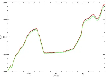
Upward and downward fluxes of longwave radiation were saved on all vertical levels in the atmosphere after the first model timestep (so that the meteorology is identical). It should be noted that species not available in HadGEM2-ES are combined into either HFC-134a or CFC-12 according to their classification. Species are combined into equivalent HFC-134a and CFC-12 by summing their radiative forcing consistently with the CMIP5 methodology. Figure 6 shows excellent agreement between the “equivalent” gases and the more detailed representation from experiments 3, 4, 5 above. Zonal mean differences are within 1 m Wm−2 everywhere
showing that the use of 2 CFC equivalent species in CMIP5 is justified.
4 Ozone
4.1 Tropospheric ozone pre-cursor emissions and concentrations
Tropospheric ozone (O3)is a significant greenhouse gas due
to its absorption in the infrared, visible, and ultraviolet spec-tral regions (Lacis et al., 1990). It has increased substan-tially since pre-industrial times, particularly in the northern mid-latitudes (e.g. Staehelin et al., 2001), which has been linked by various studies to increasing emissions of tropo-spheric O3pre-cursors: nitrogen oxides (NOx= NO + NO2),
carbon monoxide (CO), methane (CH4), and non-methane
volatile organic compounds (NMVOCs; e.g. Wang and Ja-cob, 1998). As a result, the tropospheric chemistry configu-ration of the UKCA model (O’Connor et al., 2011) was im-plemented in HadGEM2-ES and used in all CMIP5 simula-tions to simulate the time evolution of tropospheric O3
inter-actively rather than having it prescribed. The UKCA chem-istry scheme includes a description of inorganic odd oxy-gen (Ox), nitrogen (NOy), hydrogen (HOx), and CO
chem-istry with near-explicit treatment of CH4, ethane (C2H6),
propane (C3H8), and acetone (Me2CO) degradation
Fig. 6. Zonal-mean net tropopause forcing in which halocarbons controlled under the Montreal and Kyoto Protocol are represented as one equivalent species each, CFC-12 and HFC-134a, respectively (black line). The sensitivity tests with Montreal gases split into individual species (red line) and Kyoto gases split into individual species (green line) show a close agreement.
fields and lightning emissions were computed interactively. A full description and evaluation of the chemistry scheme in HadGEM2-ES can be found in O’Connor et al. (2011). Although transport and chemistry were calculated up to the model lid, boundary conditions were applied within UKCA. In the case of O3, it was overwritten in those model levels
which were 3 levels (approximately 3–4 km) above the di-agnosed tropopause (Hoerling et al., 1993) using the strato-spheric O3concentration dataset described in Sect. 4.2. It is
this combined O3field which is then passed to the model’s
radiation scheme. Furthermore, oxidation of sulphur diox-ide and dimethyl sulphdiox-ide (DMS) into sulphate aerosol (de-scribed in Sect. 5) involves hydroxyl (OH), hydroperoxyl (HO2), hydrogen peroxide (H2O2), and O3, whose
con-centrations are provided to the model’s sulphur cycle from UKCA.
No prescribed tropospheric ozone abundance data were used within HadGEM2-ES. Instead, the tropospheric evolu-tion of ozone was simulated using surface and aircraft emis-sions of tropospheric ozone precursors and reactive gases. It is these emissions, rather than tropospheric ozone concen-trations which are held constant in the pre-industrial control simulation. For the palaeoclimate simulations, the same pre-industrial emissions are also used as described in Sect. 8. For the historical and future simulations (including the emis-sions driven and decoupled carbon cycle experiments, and AMIP runs) a time-varying data set of emissions is used. As the time evolution of tropospheric ozone is simulated rather than prescribed, it may diverge from historical or RCP supplied tropospheric ozone (Lamarque et al., 2011). The emissions data used by HadGEM2-ES has been supplied for CMIP5 by Lamarque et al. (2010) and by the IAMs for the
4 RCPs. Speciated surface emissions were provided for the following sectors: land-based anthropogenic sources (agri-culture, agricultural waste burning, energy production and distribution, industry, residential and commercial combus-tion, solvent production and use, land-based transportacombus-tion, and waste treatment and disposal), biomass burning (forest fires and grass fires), and shipping. They were valid for the specific year provided with a time resolution of 10 years in the case of anthropogenic and shipping emissions but as decadal means for biomass burning. This was considered appropriate for biomass burning emissions due to their sub-stantial inter-annual variability both globally and regionally (Lamarque et al., 2010). All surface emissions were provided as monthly means on a 0.5◦×0.5◦grid. In the case of air-craft emissions, they were provided as monthly means on a 0.5◦×0.5◦ horizontal grid and on 25 levels in the vertical,
extending from the surface up to 15 km.
For the UKCA tropospheric chemistry scheme used in HadGEM2-ES, surface emissions for the following species were considered: C2H6, C3H8, CH4, CO, HCHO, Me2CO,
MeCHO, and NOx. For the CMIP5 simulations, the
spa-tially uniform surface CH4 concentration is prescribed (as
described in Sect. 3.1), and hence the surface CH4emissions
are essentially redundant in this case. For each species the provided emissions were re-gridded onto the model’s N96 grid (1.75◦×1.25◦). A small adjustment was made after re-gridding to ensure the global totals matched those of the orig-inal data.
For emissions of C2H6, it was decided to combine all
C2 species (C2H6, ethene (C2H4), and ethyne (C2H2))and
treat as emissions of C2H6. These were each converted to
kg(C2H6)m−2s−1, added together, and then regridded. For
C3H8, the C3 species (propane and propene (C3H6))were
similarly combined and treated as emissions of C3H8.
For CO, emissions from land-based anthropogenic sources, biomass burning, and shipping were taken for the historical period from Lamarque et al. (2010). These were added together and re-gridded on to an intermediate 1◦×1◦ grid in terms of kg(CO) m−2s−1. Oceanic CO emissions were also added (45 Tg(CO) yr−1), and their spatial and tem-poral distribution were provided by the Global Emissions Inventory Activity (see URL 10 in Appendix A), based on distributions of oceanic VOC emissions from Guenther et al. (1995). In the absence of an isoprene (C5H8)oxidation
mechanism in the UKCA tropospheric chemistry scheme used in HadGEM2-ES, an additional 354 Tg(CO) yr−1was
added based on a global mean CO yield of 30 % from C5H8
from a study by Pfister et al. (2008) and a global C5H8
emis-sion source of 506 TgC yr (Guenther et al., 1995). It is dis-tributed spatially and temporally using C5H8emissions from
Guenther et al. (1995) and added to the other monthly mean emissions on the 1◦×1◦grid before regridding.
the historical period and re-gridded. Similar processing was applied to the future emissions supplied by the IAMs for the 4 RCPs.
For MeCHO, the monthly mean NMVOC biomass burn-ing emissions from Lamarque et al. (2010) for the his-torical period were used. Using different emission fac-tors from Andreae and Merlet (2001) for grass fires, tropi-cal forest fires, and extra-tropitropi-cal forest fires, emissions of NMVOCs were converted into emissions of MeCHO (i.e. kg(MeCHO) m−2s−1). Surface emissions of Me2CO were
taken from land-based anthropogenic sources and biomass burning from Lamarque et al. (2010, 2011). These were added together and re-gridded on to an intermediate 1◦×1◦ grid in terms of kg(Me2CO) m−2s−1. Then, the dominant
source of Me2CO from vegetation was added, based on a
global distribution from Guenther et al. (1995) and scaled to give a global annual total of 40.0 Tg(Me2CO) yr−1. The
to-tal monthly mean emissions were then re-gridded on to the model’s N96 grid. For future emissions, the processing was identical.
Finally for NOx surface emissions, contributions from
land-based anthropogenic sources, biomass burning, and shipping from Lamarque et al. (2010) were added together and re-gridded on to an intermediate 1◦×1◦grid in terms of kg(NO) m−2s−1. Added to these were a contribu-tion from natural soil emissions, based on a global and monthly distribution provided by GEIA on a 1◦×1◦ grid (see URL 10 in Appendix A), and based on the global em-pirical model of soil-biogenic emissions from Yienger and Levy II (1995). These were scaled to contribute an additional 12 Tg(NO) yr−1. A similar approach was adopted when
pro-cessing the future emissions. All emissions provided were processed as above for the years supplied and a linear inter-polation applied between years to produce emissions for ev-ery year. Figure 7 shows the time evolution of tropospheric O3 pre-cursor surface emissions over the 1850–2100 time
period. After 2100, tropospheric ozone precursor emissions were kept constant.
In the case of NOxemissions, 3-D emissions from aircraft
were also considered. These were supplied as monthly mean fields of either NO or NO2 on a 25 level (L25) 0.5×0.5
grid by Lamarque et al. (2010) for the historical period. For HadGEM2-ES we used the NO emissions. They were first re-gridded on to an N96×L25 grid and then projected on to the model’s N96×L38 grid, ensuring that the global an-nual total emissions were conserved. A similar approach was adopted when processing the future emissions.
No additional coding in the HadGEM2-ES or UKCA mod-els was necessary for the treatment of tropospheric ozone pre-cursor emissions. The only code change was required for the Detection and Attribution “greenhouse gases only” simulation (7.2). In this case, the UKCA model was modi-fied to maintain the global mean surface CH4concentration
at pre-industrial levels i.e. 805.25 ppb. This was to ensure that the increase in CH4 concentration as seen by the
radi-ation scheme did not affect concentrradi-ations of tropospheric oxidants, thereby influencing the rate of sulphate aerosol for-mation.
4.2 Stratospheric ozone concentration
HadGEM2-ES requires stratospheric ozone to be input as monthly zonal/height ancillary files. CMIP5 recommends the use of the AC&C/SPARC ozone database (Cionni et al., 2011) which covers the period 1850 to 2100 and can be used in climate models that do not include interactive chemistry. The pre-industrial dataset consists of a repeating seasonal cy-cle of ozone values, and this is also used for the palaeocli-mate simulations described in Sect. 8. For the historical and future simulations (including the emissions driven and de-coupled carbon cycle experiments, and AMIP runs) a time-varying data set of stratospheric ozone is used.
The historical part of the AC&C/SPARC ozone database spans the period 1850 to 2009 and consists of separate strato-spheric and tropostrato-spheric data sources. The future part of the AC&C/SPARC ozone database covers the period 2010 to 2100 and seamlessly extends the historical database also in-cluding separate stratospheric and tropospheric data sources based on 13 CCMs that performed a future simulation until 2100 under the SRES A1B GHG scenario.
The AC&C/SPARC ozone is provided on pressure levels between 1000-1 hPa. The UK National Centre for Atmo-spheric Science (NCAS) has produced an updated version of the SPARC ozone dataset as follows.
A multiple-linear regression was performed on the his-torical raw pressure-level data between 1000-1 hPa consis-tent with the Randel and Wu (1999) method used to con-struct the timeseries. The ozone was then represented as: O3(t )=a∗SOL +b∗EESC + seasonal cycle + residuals. For
consistency, the indices of 11-yr solar cycle (SOL) and total equivalent chlorine (EESC) are identical to those used to pre-pare the original dataset. The SOL index is a 180.5 nm time-series provided by Fei Wu at NCAR. The standard SPARC ozone dataset which extends into the future does not include solar cycle variability post-2009. For production of a dataset extending into the future including an 11-yr ozone solar cy-cle, the solar regression index is used to build a future time series consistent with a repeating solar irradiance compiled by the Met Office Hadley Centre (see Sect. 7.1) and is mod-elled as a sinusoid with a period of 11 yr, with mean and max-min values corresponding to solar cycle 23 normalised against the 180.5 nm timeseries used in the historical ozone. There is no solar ozone signal in the high latitudes.
Fig. 7.Tropospheric ozone pre-cursor surface emissions over the historical period (1850–2005) and over the future period (2005–2100) from the 4 RCPs: RCP3-PD (blue), RCP4.5 (green), RCP6 (yellow), and RCP8.5 (red). The methane (CH4)emissions shown do not include a
contribution from wetlands.
5 Tropospheric aerosol forcing
HadGEM2-ES simulates concentrations of six tropospheric aerosol species: ammonium sulphate, fossil-fuel black car-bon, fossil-fuel organic carcar-bon, biomass-burning, sea-salt, and mineral dust aerosols (Bellouin et al., 2007; Collins et al., 2011). Although an ammonium nitrate aerosol scheme is available to HadGEM2-ES, it was still in its developmen-tal version when CMIP5 simulations started, hence nitrate aerosols are not included in the CMIP5 simulations. In addi-tion, secondary organic aerosols from biogenic emissions are represented by a fixed climatology. All aerosol species can exert a direct effect by scattering and absorbing shortwave and longwave radiation, and a semi-direct effect whereby this direct effect modifies atmospheric vertical profiles of tem-perature and clouds. In HadGEM2-ES all aerosol species, except fossil-fuel black carbon and mineral dust, also con-tribute to both the first and second indirect effects on clouds, modifying cloud albedo and precipitation efficiency, respec-tively. Changes in direct and indirect effects since 1860 are termed aerosol radiative forcing. The magnitude of this
forcing depends on changes in aerosols, which are due in part to changes in emissions of primary aerosols and aerosol pre-cursors. Changes in emission rates are either derived from external datasets or due to changes in the simulated climate. Here we document how any changes in emission rates are implemented in the HadGEM2-ES CMIP5 centennial exper-iments. In the control run we specify a repeating seasonal cycle of 1860 emissions, and this is also used in the palaeocli-mate simulations (Sect. 8). Historical and future simulations (including the emissions-driven and decoupled carbon cycle experiments and AMIP runs) use time-varying emissions as described in this section.
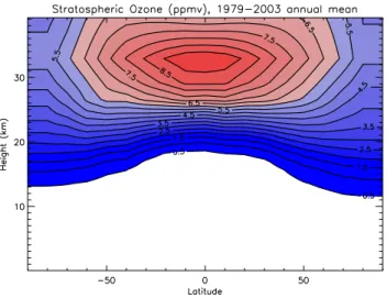
Fig. 8. Annual mean climatology of ozone volume mixing ration (ppmv) for 1979–2003.
precursors and primary aerosols are not included in the model.
The sulphur cycle, which provides concentrations of ammonium sulphate aerosols, requires emissions of sul-phur dioxide (SO2)and dimethyl-sulphide (DMS). Sulphur
dioxide emissions are derived from sector-based emissions. Emissions for all sectors are injected at the surface, except for energy emissions and half of industrial emissions which are injected at 0.5 km to represent chimney-level emissions. Sulphur dioxide emissions from biomass burning are not in-cluded. The model accounts for three-dimensional back-ground emissions of sulphur dioxide from degassing volca-noes, taken from Andres and Kasgnoc (1998). This rep-resents a constant rate of 0.62 Tg[S] yr−1 on a global
av-erage, independent of the year simulated and is not part of the implementation of volcanic climate forcing which we discuss in Sect. 7.2. Similarly, land-based DMS emis-sions do not vary in time and give 0.86 Tg yr−1 (Spiro et al., 1992). Oceanic DMS emissions are provided interac-tively by the biogeochemical scheme of the ocean model as a function of local chlorophyll concentrations and mixed layer depth (based on Simo and Dachs, 2002). In an objective assessment against ship-board and time-series DMS obser-vations, the HadGEM2-ES interactive ocean DMS scheme performs with similar skill to that found in the widely used Kettle et al. (1999) climatology (Halloran et al., 2010). The primary differences between the model-simulated and the climatology-interpolated surface ocean DMS fields are; lower model Southern Hemisphere summer Southern Ocean DMS concentrations, higher model annual equatorial DMS concentrations, and a reduced model seasonal cycle ampli-tude. Oxidation of sulphur-dioxide and DMS into sulphate aerosol involves hydroxyl (OH), hydroperoxyl (HO2),
hy-drogen peroxide (H2O2), and ozone (O3): concentrations for
those oxidants are provided by the tropospheric chemistry scheme.
Fig. 9. Timeseries of column ozone (in Dobson Units, DU) for global annual mean (black line), 60◦S–90◦S September– November mean (red line) and 60◦N–90◦N February–April mean (blue line).
Emissions of primary black and organic carbon from fossil fuel and biofuel are injected at 80 m. Emissions of biomass-burning aerosols are the sum of the biomass-biomass-burning emis-sions of black and organic carbon. Grassfire emisemis-sions are assumed to be located at the surface, while forest fire emis-sions are injected homogeneously across the boundary layer (0.8 to 2.9 km).
Sea-salt emissions are computed interactively over open oceans at each model time step from near-surface (10 m) wind speeds (Jones et al., 2001). Mineral dust emissions are also interactive, and depend on near-surface wind speed, land cover and soil properties. The scheme is described in Woodward (2011). It is based on that designed for HadAM3 (Woodward, 2001) with major developments including the modelling of particles up to 2 mm in the horizontal flux, threshold friction velocities based on Bagnold (1941), a mod-ified version of the F´ecan et al. (1999) soil moisture treatment and the utilisation of a preferential source multiplier similar to that described in Ginoux et al. (2001).
Finally, secondary organic aerosols from biogenic emis-sions are represented by monthly distributions of three-dimensional mass-mixing ratios obtained from a chemistry transport model (Derwent et al., 2003). These distributions are constant for all simulated years.
6 Land-use and land-use change
Emissions of sulphur dioxide
1850 1900 1950 2000 2050 2100 Year 0 20 40 60 80 Tg[S]/yr Historical RCP3-PD RCP4.5 RCP6.0 RCP8.5
Emissions of ammonia
1850 1900 1950 2000 2050 2100 Year 10 20 30 40 50 60 70 80 Tg[N]/yr Historical RCP3-PD RCP4.5 RCP6.0 RCP8.5
Emissions of fossil-fuel black carbon
1850 1900 1950 2000 2050 2100 Year 1 2 3 4 5 6 7 Tg[C]/yr Historical RCP3-PD RCP4.5 RCP6.0 RCP8.5
Emissions of fossil-fuel organic carbon
1850 1900 1950 2000 2050 2100 Year 2 4 6 8 10 12 14 16 Tg[C]/yr Historical RCP3-PD RCP4.5 RCP6.0 RCP8.5
Emissions of biomass-burning aerosol
1850 1900 1950 2000 2050 2100 Year 15 20 25 30 35 Tg[C]/yr Historical RCP3-PD RCP4.5 RCP6.0 RCP8.5
Land-based emissions of DMS
1850 1900 1950 2000 2050 2100 Year 0.0 0.2 0.4 0.6 0.8 1.0 Tg[S]/yr Historical RCP3-PD RCP4.5 RCP6.0 RCP8.5
Fig. 10. Tropospheric aerosol precursors and aerosol primary emissions over the historical period (1860–2005), and future period (2005– 2100) for 4 RCPs: RCP3-PD (blue), RCP4.5 (green), RCP6.0 (yellow), RCP8.5 (red).
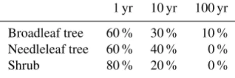
condition to the dynamic vegetation scheme. Previous Met Office Hadley Centre coupled climate-carbon cycle simula-tions (e.g. Cox et al., 2000; Freidlingstein et al., 2006) used a static (present day) agricultural mask. However the dy-namic vegetation scheme, TRIFFID has now been updated to allow time-varying land-use distributions in the CMIP5 simulations.
TRIFFID represents the fractional coverage in each grid cell of 5 plant functional types (PFTs: broadleaf tree, needle-leaf tree, C3 grass, C4 grass, shrub) and also bare soil. Pre-scribed fractions of urban areas, lakes and ice are also in-cluded from the IGBP land cover map (Loveland et al., 2000) and do not vary in time. The summed fractional coverage of crop and pasture is provided as a time-varying input. Within a grid box tree and shrub PFTs are excluded from this frac-tion allowing natural grasses to grow and represent “crops”. Abandonment of crop land removes this constraint on trees and shrubs but we do not specify instant replacement by these woody PFTs, but rather their regrowth is simulated by the model’s vegetation dynamics. If woody vegetation cover re-duces because of a land use change, vegetation carbon from the removed woody PFTs goes partially to the soil carbon
Table 3.Allocation of aboveground displaced carbon to the differ-ent wood products pools, based on the values given in McGuire et al. (2001, Table 3) but recalculated to be applied to just the above-ground carbon flux.
1 yr 10 yr 100 yr
Broadleaf tree 60 % 30 % 10 % Needleleaf tree 60 % 40 % 0 %
Shrub 80 % 20 % 0 %
HadGEM2-ES is therefore able to simulate both biophysi-cal and biogeochemibiophysi-cal effects of land-use change as well as natural changes in vegetation cover in response to changing climate and CO2. In this version of the model only
anthro-pogenic disturbance in the form of crop and pasture is rep-resented. Data on within-grid-cell transitions due to shifting cultivation or the impact of wood harvest are not yet used. As described in Sect. 2.2, CO2emissions from land-use change
can be simulated by HadGEM2-ES but are not used interac-tively in the emissions driven experiment.
The biophysical impacts of land use change include the di-rect effect of changes to surface albedo and roughness due to land-cover change and also changes to the hydrological cy-cle due to changes in evapotranspiration and runoff. There is also an indirect physical effect due to changes in surface emissions of mineral dust caused by changes in bare soil frac-tion, windspeed and soil moisture, which has a radiative ef-fect in the atmosphere.
Historic and future simulations (including the emissions-driven and decoupled carbon cycle simulations and AMIP runs) use time varying disturbance from the Hurtt et al. (2011) dataset described below. The pre-industrial con-trol simulation uses an agricultural disturbance mask, fixed in time at 1860 values in this same dataset. The natural and GHG detection and attribution simulations (7.1, 7.2) also use a fixed, pre-industrial land-use disturbance mask, but the land-use only simulations (7.3) use the time varying histor-ical data as in the full historhistor-ical simulation. For the mid-Holocene and LGM experiments, there is no agricultural dis-turbance (which therefore differs from the control run where a pre-industrial disturbance mask is used). The Last Millen-nium and AMIP simulations do not use the dynamic vegeta-tion scheme of HadGEM2-ES and instead directly prescribe land-cover as described in Sects. 8 and 9, respectively.
The historical land use data is based on the HYDE database v3.1 (Klein Goldewijk et al., 2010, 2011), whilst the future RCP land use scenarios were produced by the respective IAMs and are thus internally consistent with the socio-economic storylines and carbon emissions of the sce-narios. A harmonization manipulation was performed, as described in Hurtt et al. (2009, 2011), that attempts to pre-serve gridded and regional IAM crop and pasture changes as much as possible while minimizing the differences in 2005 between the historical estimates and future projections (Fig. 11). The harmonization procedure employs the Global Land-use Model (GLM) that ensures a smooth and consis-tent transition in the harmonization year, grids (or re-grids) the data when necessary, spatially allocates national/regional wood harvest statistics, and computes all the resulting land-use states and transitions between land-land-use states annually from 1500–2100 at half-degree (fractional) spatial resolu-tion, including the effects of wood harvesting and shifting cultivation. Both historical and future scenarios were made available at 0.5◦×0.5◦ resolution with annual increments and were downloaded (see URL 11 in Appendix A).
Fig. 11.Fractional coverage of anthropogenic disturbance, defined as the sum of crop and pasture, for the historical period 1860–2005, and up to 2100 following the 4 RCP scenarios, RCP3-PD (blue), RCP4.5 (green), RCP6 (yellow) and RCP8.5 (red).
The crop and pasture fraction is re-gridded onto the HadGEM2-ES grid using area average re-gridding. Crop and pasture are then combined to produce a combined “agricul-ture” mask (Fig. 12). It is assumed crop and pasture both mean “only grass, no tree or shrub”. This assumption is simplistic as in some regions of the world “pasture” refers to rangeland where animals are allowed to graze on what-ever natural vegetation exists there (which may include trees and shrub). Similarly, woody biofuel crops are treated (er-roneously in this case) as non-woody crops. As noted by Hurtt et al. (2011), the definition and reporting of biofuel differs even within the IAMs producing the 4 RCP scenarios. However, the necessary data to avoid these problems are not available and we expect the impact of any inconsistency to be minor. It remains an outstanding research activity to im-prove past and present reconstructions of land-cover which can account for temporally and regionally varying changes in definitions and terminology.
Our approach of allocating displaced woody biomass into product pools which subsequently release CO2to the
atmo-sphere means that our definition of “land use CO2flux” that
Fig. 12. Historical land use presented as fractional anthropogenic disturbance at(a)1860 and(b)2005.
analysing land-use emissions from such models, or compar-ing between different models or techniques that the precise methodology is described to avoid misunderstanding. It re-mains a research priority to formally define methodologies for reporting simulated land-use fluxes.
An additional uncertainty in reporting the land use car-bon fluxes is that the wood products pools are assumed to be zero everywhere at 1860 whilst the terrestrial carbon cy-cle (carbon content and vegetation fractions) have been run to equilibrium with 1860 climate and anthropogenic distur-bance. Changes in land use cover prior to 1860 involve land use expansion and hence both direct emissions prior to 1860 and some legacy emissions post-1860 due to inputs of dis-turbed biomass to the soil carbon. No attempt has been made to include these effects in our output but future work will assess and quantify this effect.
7 Natural climate forcing
HadGEM2-ES can simulate the climate response to two as-pects of natural climate forcing: changes in solar irradiance and stratospheric volcanic aerosol. In the control experiment
these forcings are kept constant in time. For the historical experiments (including the emissions-driven and decoupled carbon cycle simulations and AMIP runs) they are varied due to observed reconstructions. For simulations of future peri-ods, where natural forcings are not known, they are varied as described here to minimise the impact of possibly incorrect assumptions about the natural forcings. See Sect. 8 for de-tails on the solar and volcanic forcings applied to the palaeo-climate simulations.
7.1 Total solar irradiance
The way the model deals with variations in total solar irra-diance (TSI) is the same as in earlier generations of Hadley Centre models, HadCM3 (Stott et al., 2000; Tett et al., 2002) and HadGEM1 (Stott et al., 2006). Annual mean variations in TSI are partitioned across the six shortwave spectral bands (0.2–10 µm) to estimate the associated spectral changes with TSI variations (Lean et al., 1995a). With the changes across the spectral bands the Rayleigh scattering and ozone absorp-tion properties are also varied. See Stott et al. (2006) for further details.
The TSI data used for the historic period were recom-mended by CMIP5 (Lean et al., 2009 -L09) and are cre-ated from reconstructions of solar cycle and background variations in TSI. The solar cycle component is produced from a multiple regression of proxy measures of bright and dark regions of the Sun with satellite reconstructions of TSI (Fr¨ohlich and Lean, 2004). Background variations in TSI are produced from a model of solar magnetic flux incorporating historic sunspot numbers (Wang et al., 2005). The annual mean TSI was processed to force the mean of the 1700–2004 period to be the same as the model control solar constant value (1365 Wm−2).
The annual mean TSI and variations across the UV, vis-ible and IR bands are shown in Fig. 13. For comparison the TSI used in previous model simulations are also shown. The TSI now recommended for use in CMIP5 studies is con-sistent with the latest assessment of TSI variations by the IPCC’s Fourth Assessment report – AR4 – (Forster et al., 2007) which estimated the solar radiative forcing to be 50 % of that given in the previous report. The increase in TSI for L09 between the Maunder minimum in the 17th century and the average over the last 2 solar cycles of the 20th century is 1.11 Wm−2. This compares to 2.73 Wm−2 for the TSI used in the HadGEM1 simulations (Stott et al., 2006) and 2.95 Wm−2in the HadCM3 simulations (Stott et al., 2000). 7.2 Stratospheric volcanic aerosol
How HadGEM2-ES incorporates changes in stratospheric volcanic aerosol is the
TSI
1850 1900 1950 2000
Date 1365 1366 1367 Wm -2 TSI
1850 1900 1950 2000
Date -0.05 0.00 0.05 0.10 0.15 0.20 Percentage LBB95 SK03 L09 UV
1850 1900 1950 2000
Date 29.2 29.3 29.4 29.5 Wm -2 UV
1850 1900 1950 2000
Date -0.2 0.0 0.2 0.4 0.6 0.8 Percentage Visible
1850 1900 1950 2000
Date 594.5 595.0 595.5 Wm -2 Visible
1850 1900 1950 2000
Date 0.00 0.05 0.10 Percentage IR
1850 1900 1950 2000
Date 740.8 741.0 741.2 741.4 Wm -2 IR
1850 1900 1950 2000
Date -0.02 0.00 0.02 0.04 0.06 0.08 Percentage
Fig. 13.Annual mean solar irradiance variations used in the historic model simulation (L09 - Lean et al., 2009). (a)Total solar irradi-ance. Also shown are the TSI used in previous model simulations, LBB95 (Lean et al., 1995b) used in HadCM3 (Stott et al., 2000) and SK03 (Solanki and Krivova, 2003) used in HadGEM1 (Stott et al., 2006). Solar irradiance averaged over(b)the ultraviolet band (200– 320 nm),(c)the two visible bands (320–690 nm), and(d)infrared bands (690–1190, 1190–2380, and 2380–10 000 nm). Percentages are given with respect to the solar constant (1365 Wm−2), and as-sociated distribution across the shortwave spectral bands.
stratosphere are separated from these processes and are prescribed. Stratospheric aerosol concentrations are var-ied across four equal area latitudinal zones on a monthly timescale. The aerosol is distributed vertically above the tropopause such that the mass mixing ratio is constant across the levels. In this version of the model, volcanic aerosol is not related to, and does not interact with, other simulated aerosol behaviour.
The dataset used for the historic period was monthly stratospheric optical depths, at 550 nm, from 1850 to 2000 (Sato et al., 1993, see URL 12 in Appendix A) which was averaged over the four equal area latitudinal zones and con-verted into aerosol concentrations (Stott et al., 2006 and fig-ures therein).
In a previous study (Stott et al., 2006) the data was ex-tended past 2000 by continuing an assumed 1 yr timescale decay, from 1997, to a minimum and then keeping con-centrations constant. There is some evidence that back-ground aerosol concentrations are not as low as this as-sumes (Thomason et al., 2008). Also future volcanic
Global mean optical depth
1990 2000 2010 2020 2030 2040
1 10 100 1000
optical depth x 10000.
This study Stott 2006 study
Fig. 14. Monthly global mean stratospheric optical depth as used in this study and what was included in the HadGEM1 simulations (Stott, 2006), for the period 1990–2040.
activity is likely to introduce further aerosol into the strato-sphere. There was no specific CMIP5 recommendations, apart from suggesting that the same concentration of strato-spheric aerosol is present in the future simulations as in the control (Taylor et al., 2009), being aware of any step-change in aerosol.
The future dataset of optical depth is constructed as fol-lows. The 1 yr decay timescale constructed for the post 1997 period appears to give a break point in the data. We re-construct the data, to remove the break point, from 1997 to 2002 by continuing the decay timescale of 3.3 yr seen in the 1995–1997 period of the data. A value of stable observed optical depth at 1020 nm since 2000 was found to be 0.001 (Thomason et al., 2008). As optical depth is estimated to vary inversely with wavelength, this suggests a minimum of global stratospheric aerosol optical depth of 0.002 at 550 nm, approximately 20 times more than used in the HadGEM1 study. During the period 2020–2040 concentrations were increased to match those in the control simulation (optical depth 0.0097). This compromise was an attempt to balance the lack of knowledge of when large eruptions would occur in the future with the unlikely possibility of no major vol-canic eruptions significantly influencing aerosol amounts in the stratosphere for 100 yr. The global mean of the strato-spheric optical depth is shown in Fig. 14, compared with what was used in the HadGEM1 simulation.
8 Palaeoclimate boundary conditions, including geophysical changes
In order to complete the palaeo-climate simulations (3.4–3.6) a number of modifications need to be made to the model. The mid-Holocene simulation (3.4) required GHG concen-trations of CH4(650 ppb) and N2O (270 ppb), and
Fig. 15. Mid-Holocene changes in monthly TOA solar insolation relative to the present day, as a function of latitude as supplied by PMIP3 and calculated within HadGEM2-ES.
simulation). Stratospheric Ozone and pre-cursor emissions of tropospheric ozone remain the same as the pre-industrial control run, as do concentrations of CO2 and the land sea
mask. Because tropospheric Ozone is calculated interac-tively in HadGEM2-ES, Ozone concentrations in the palaeo simulations may not be identical to those in the pre-industrial control simulation: it is the pre-cursor emissions which we keep the same as the control run. This is also the case for dust and ocean DMS emissions which are simulated interac-tively and may differ due to changes in the simulated climate or vegetation cover.
8.1 Mid-Holocene (6 kya)
In the mid-Holocene, Earth’s orbit differed from present day affecting the timing and magnitude of solar energy reach-ing the surface. Orbital parameters were modified to corre-spond to those required by the PMIP3 protocol (see URL 13 in Appendix A). Figure 15 shows the monthly anomalies of
Fig. 16.Land sea masks used by HadGEM2-ES. Modern and mid-Holocene land points are denoted by white and additional LGM land points by grey. Black points denote points that are ocean in all simulations.
TOA SW radiation relative to the present day for the offi-cial PMIP3 requirements (black) and as calculated within HadGEM2-ES (red). The land use disturbance mask is set to zero everywhere for the mid-Holocene thus assuming that there is no human activity which would displace forests in any location.
8.2 Last glacial maximum (LGM, 21 kya)
The LGM simulation (3.5) setup requires major changes to the geophysical state of the land and ocean bed. This sim-ulation has not yet been performed and some of these mod-ifications are ongoing. The land sea mask and orography are changed to increase ice sheet volumes and to represent the associated decreased sea level. The bathymetry of the ocean model is also changed to reflect the decreased sea-level. Figure 16 shows how the land-sea mask changes. GHG concentrations are prescribed as, CO2 of 185 ppm, CH4 of
350 ppb, N2O of 200 ppb. Halocarbons are zero (as in the
pre-industrial control setup) and O3 is treated the same as
in the pre-industrial control run by using the same strato-spheric ozone concentrations and tropostrato-spheric ozone pre-cursor emissions. Boundary condition files were downloaded from the PMIP3 website (see URL 13 in Appendix A). Or-bital parameters will be changed to the required configuration and the river routing ancillary will also be manually updated to take into account changes in the land sea mask and ensure that all rivers flow into the ocean rather than terminating at a land-point.
8.3 Last Millennium (800 AD–present)
Table 4.Mapping of the P08 land classes into HadGEM2-ES veg-etation types.
Classification Classification
in P08 in MOSES2
Tropical evergreen forest Broadleaf trees
Tropical deciduous forest Broadleaf trees
Temperate evergreen broadleaf forest Broadleaf trees Temperate/boreal deciduous broadleaf forest Broadleaf trees Temperate/boreal evergreen conifers Needle leaf trees Temperate/boreal deciduous conifers Needle leaf trees
Raingreen shrub Shrubs
Summergreen shrub Shrubs
C3 natural grasses C3 grasses
C4 natural grasses C4 grasses
Tundra multiple mapping
Crop multiple mapping
C3 pasture C3 grasses
C4 pasture C4 grasses
to year 800 AD. The vegetation types in the P08 database are mapped into the 5 TRIFFID vegetation classes. The details of the reclassification are shown in Table 4. In case of no one-to-one mapping, the following rules are applied:
– C3/C4 pasture is treated as natural C3/C4 grass. – Tundra is treated as mixture of shrubs, grass and bare
soil. The mixture is chosen to match as close as possible the distribution obtained in Essery et al. (2003) in tundra regions for the present time.
– Crops are treated as in Essery et al. (2003), as a mixture of C3/C4 grass and soil. The ratio between C3 and C4 grass is used as threshold to discriminate between C3 and C4 grass to be used in crop.
After the application of inland water mask and ice mask, the unclassified fraction of each grid cell is filled with the soil land class. For the urban land class we used the data from HYDE3.1 (Klein Goldewijk et al., 2010, 2011). The data provide the urban/built-up area on a grid cell of 0.083◦×0.083◦. We used local area-averaging interpolation to regrid HYDE 3.1 data into the P08 grid. In the coastal areas only the grid cells where at least 30 % of the origi-nal data showed urban coverage were considered as urban. The half-degree historical land cover data is then re-gridded onto the HadGEM2-ES grid using area average re-gridding. Figure 17 shows the total woodland (needle leaf+broad leaf trees) reduction with respect to year 800 respectively in year 1000, 1500 and 1990 on the HadGEM2 grid.
For the volcanic forcing we use the reconstruction of aerosol optical depth (AOD) provided by Crowley et al. (2008) and we maintain the same latitudinal distribution as described in Sect. 7.2. The reconstruction is based on ice-core records from Antarctic and Greenland calibrated based
Fig. 17. Changes in fractional area coverage of woodland (broad leaf+needle leaf tree) in year 1000 AD, 1500 AD and 1990 AD with respect to the year 800 AD. Data from Pongratz et al. (2008) regrid-ded on HadGEM2-ES grid.
on the Pinatubo eruption and is validated by comparison to the 20th century instrumental records. The data closely match the Sato et al. (1993) reconstruction for the 20th cen-tury. Figure 18 shows the volcanic aerosol optical depth at 0.55 µm integrated across the lower stratosphere between 15 and 25 km for the 4 latitudinal bands from the year 800 to 2000.