The HadGEM2-ES implementation of CMIP5 centennial simulations

(1)

GMDD

4, 689–763, 2011

The HadGEM2-ES implementation of CMIP5 centennial

simulations

C. D. Jones et al.

Title Page

Abstract Introduction

Conclusions References

Tables Figures

◭ ◮

Back Close

Full Screen / Esc

Printer-friendly Version Interactive Discussion

Discussion

P

a

per

|

Dis

cussion

P

a

per

|

Discussion

P

a

per

|

Discussio

n

P

a

per

|

Geosci. Model Dev. Discuss., 4, 689–763, 2011 www.geosci-model-dev-discuss.net/4/689/2011/ doi:10.5194/gmdd-4-689-2011

Geoscientific Model Development Discussions

This discussion paper is/has been under review for the journal Geoscientific Model Development (GMD). Please refer to the corresponding final paper in GMD if available.

The HadGEM2-ES implementation of

CMIP5 centennial simulations

C. D. Jones1, J. K. Hughes1, N. Bellouin1, S. C. Hardiman1, G. S. Jones1, J. Knight1, S. Liddicoat1, F. M. O’Connor1, R. J. Andres2, C. Bell3,†, K.-O. Boo4, A. Bozzo5, N. Butchart1, P. Cadule6, K. D. Corbin7,*, M. Doutriaux-Boucher1, P. Friedlingstein8, J. Gornall1, L. Gray9, P. R. Halloran1, G. Hurtt10,16,

W. Ingram1,11, J.-F. Lamarque12, R. M. Law7, M. Meinshausen13, S. Osprey9, E. J. Palin1, L. Parsons Chini10, T. Raddatz14, M. Sanderson1, A. A. Sellar1, A. Schurer5, P. Valdes15, N. Wood1, S. Woodward1, M. Yoshioka15, and M. Zerroukat1

1

Met Office Hadley Centre, Exeter, EX1 3PB, UK 2

Environmental Sciences Division, Oak Ridge National Laboratory, Oak Ridge, TN 37831-6335, USA

3

Meteorology Dept, University of Reading, Reading, RG6 6BB, UK 4

National Institute of Meteorological Research, Korea Meteorological Administration, Korea 5

School of GeoSciences, University of Edinburgh, The King’s Buildings, Edinburgh EH9 3JW, UK

6

(2)

GMDD

4, 689–763, 2011

simulations

C. D. Jones et al.

Title Page

Tables Figures

◭ ◮

Back Close

Full Screen / Esc

Discussion

P

a

per

|

Dis

cussion

P

a

per

|

Discussion

P

a

per

|

Discussio

n

P

a

per

|

7

Centre for Australian Weather and Climate Research, CSIRO Marine and Atmospheric Research, Aspendale, Victoria, Australia

8

College of Engineering, Mathematics and Physical Sciences, University of Exeter, Exeter, EX4 4QF, UK

9

National Centre for Atmospheric Science, Department of Physics, University of Oxford, Oxford, OX1 3PU, UK

10

Department of Geography, University of Maryland, College Park, MD 21403, UK 11

Department of Physics, University of Oxford, Oxford, OX1 3PU, UK 12

Atmospheric Chemistry Division, UCAR, Boulder, USA 13

Earth System Analysis, Potsdam Institute for Climate Impact Research, Germany 14

Max Planck Institute for Meteorology, Hamburg, Germany 15

School of Geographical Sciences, University of Bristol, Bristol BS8 1SS, UK 16

Pacific Northwest National Laboratory, Joint Global Change Research Institute, University of Maryland, College Park, MD 20740, USA

∗

now at: Colorado State University, Fort Collins, USA

†

deceased, 20 June 2010

Received: 7 March 2011 – Accepted: 16 March 2011 – Published: 31 March 2011

Correspondence to: C. D. Jones (chris.d.jones@metoffice.gov.uk)

(3)

GMDD

4, 689–763, 2011

simulations

C. D. Jones et al.

Title Page

Tables Figures

◭ ◮

Back Close

Full Screen / Esc

Discussion

P

a

per

|

Dis

cussion

P

a

per

|

Discussion

P

a

per

|

Discussio

n

P

a

per

|

Abstract

The scientific understanding of the Earth’s climate system, including the central ques-tion of how the climate system is likely to respond to human-induced perturbaques-tions, is comprehensively captured in GCMs and Earth System Models (ESM). Diagnosing the

simulated climate response, and comparing responses across different models, is

cru-5

cially dependent on transparent assumptions of how the GCM/ESM has been driven – especially because the implementation can involve subjective decisions and may dif-fer between modelling groups performing the same experiment. This paper outlines

the climate forcings and setup of the Met Office Hadley Centre ESM, HadGEM2-ES

for the CMIP5 set of centennial experiments. We document the prescribed

green-10

house gas concentrations, aerosol precursors, stratospheric and tropospheric ozone assumptions, as well as implementation of land-use change and natural forcings for the HadGEM2-ES historical and future experiments following the Representative Con-centration Pathways. In addition, we provide details of how HadGEM2-ES ensemble members were initialised from the control run and how the palaeoclimate and AMIP

15

experiments, as well as the “emission-driven” RCP experiments were performed.

1 Introduction

Phase 5 of the Coupled Model Intercomparison Project (CMIP5) is a standard experi-mental protocol for studying the output of coupled ocean-atmosphere general circula-tion models (GCMs). It provides a community-based infrastructure in support of climate

20

model diagnosis, validation, intercomparison, documentation and data access. The purpose of these experiments is to address outstanding scientific questions that arose as part of the IPCC Fourth Assessment report (AR4) process, improve understanding of climate, and to provide estimates of future climate change that will be useful to those

considering its possible consequences and the effect of mitigation strategies.

25

(4)

GMDD

4, 689–763, 2011

simulations

C. D. Jones et al.

Title Page

Tables Figures

◭ ◮

Back Close

Full Screen / Esc

Discussion

P

a

per

|

Dis

cussion

P

a

per

|

Discussion

P

a

per

|

Discussio

n

P

a

per

|

the IPCC Fifth Assessment Report (AR5) as well as others that extend beyond the AR5. The IPCC’s AR5 is scheduled to be published in September 2013. CMIP5 promotes a standard set of model simulations in order to:

– evaluate how realistic the models are in simulating the recent past,

– provide projections of future climate change on two time scales, near term (out to

5

about 2035) and long term (out to 2100 and beyond), and

– understand some of the factors responsible for differences in model projections,

including quantifying some key feedbacks such as those involving clouds and the carbon cycle.

A much more detailed description can be found on the CMIP5 project webpages (see

10

URL 1 in Appendix A) and in Taylor et al. (2009).

There are a number of new types of experiments proposed for CMIP5 in comparison with previous incarnations. As in previous intercomparison exercises, the main

fo-cus and effort rests on the longer time-scale (“centennial”) experiments, including now

emission-driven runs of models that include a coupled carbon-cycle (ESMs). These

15

centennial experiments are being performed at the Met Office Hadley Centre with the

HadGEM2-ES Earth System model (Collins et al., 2011; Martin et al., 2011); a

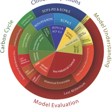
config-uration of the Met Office’s Unified Model. Figure 1 outlines the main experiments and

groups them into categories: “realistic” above the line (with studies of the past to the left and future projections to the right) and “idealised” or process-understanding

stud-20

ies below the line. The central pink area shows simulations regarded as “core” with the priority nominally decreasing to tier-1 (yellow) and then tier-2 (green).

In the following, we briefly describe HadGEM2-ES ESM, which is documented in detail in Collins et al. (2011). HadGEM2-ES is a coupled AOGCM with atmospheric

resolution of N96 (1.875◦×1.25◦) with 38 vertical levels and an ocean resolution of 1◦

25

(increasing to 1/3◦ at the equator) and 40 vertical levels. HadGEM2-ES also

(5)

GMDD

4, 689–763, 2011

simulations

C. D. Jones et al.

Title Page

Tables Figures

◭ ◮

Back Close

Full Screen / Esc

Discussion

P

a

per

|

Dis

cussion

P

a

per

|

Discussion

P

a

per

|

Discussio

n

P

a

per

|

to prescribe either atmospheric CO₂concentrations or to prescribe anthropogenic CO₂

emissions and simulate CO2concentrations as described in Sect. 2. An interactive

tro-pospheric chemistry scheme is also included, which simulates the evolution of atmo-spheric composition and interactions with atmoatmo-spheric aerosols. The model timestep is 30 min (atmosphere and land) and 1 h (ocean). Extensive diagnostic output is being

5

made available to the CMIP5 multi-model archive. Output is available either at certain prescribed frequencies or as time-average values over certain periods as detailed in the CMIP5 output guidelines (see URL 2 in Appendix A).

The CMIP5 simulations include 4 future scenarios referred to as “Representative Concentration Pathways” or RCPs (Moss et al., 2010). These future scenarios have

10

been generated by four integrated assessment models (IAMs) and selected from over 300 published scenarios of future greenhouse gas emissions resulting from socio-economic and energy-system modelling. These RCPs are labelled according to the approximate global radiative forcing level in 2100 for RCP8.5 (Riahi et al., 2007), dur-ing stabilisation after 2150 for RCP4.5 (Clarke et al., 2007; Smith and Wigley, 2006)

15

and RCP6 (Fujino et al., 2006) or the point of maximal forcing levels in the case RCP3-PD (van Vuuren et al., 2006, 2007), with RCP3-PD standing for “Peak and Decline”. The latter scenario has previously been known as RCP2.6, as radiative forcing levels decline

to-wards 2.6 Wm−2 by 2100. Note that these radiative forcing levels are illustrative only,

because greenhouse gas concentrations, aerosol and tropospheric ozone precursors

20

are prescribed, resulting in a wide spread in radiative forcings across different models.

The experimental protocol involves performing a historical simulation (defined for HadGEM2-ES as 1860 to 2005) using the historical record of climate forcing factors such as greenhouse gases, aerosols and natural forcings such as solar and volcanic changes. The model state at 2005 is then used as the initial condition for the 4 future

25

(6)

GMDD

4, 689–763, 2011

simulations

C. D. Jones et al.

Title Page

Tables Figures

◭ ◮

Back Close

Full Screen / Esc

Discussion

P

a

per

|

Dis

cussion

P

a

per

|

Discussion

P

a

per

|

Discussio

n

P

a

per

|

Many of these experiments require technical implementation by means of either or both of the following:

– time-varying boundary conditions such as concentrations of greenhouse gases

or emissions of reactive chemical species or aerosol pre-cursors. These may be given as single, global-mean numbers, or supplied as 2-D or 3-D fields of data,

5

– code changes to alter the scientific behaviour of the model, such as to

decou-ple various feedbacks and interactions (e.g. the “uncoudecou-pled” carbon cycle experi-ments).

This paper presents in detail the technical aspects of how these model forcings are implemented in HadGEM2-ES. It is not our intention here to present scientific results

10

from the experiments. This analysis will be left for subsequent work.

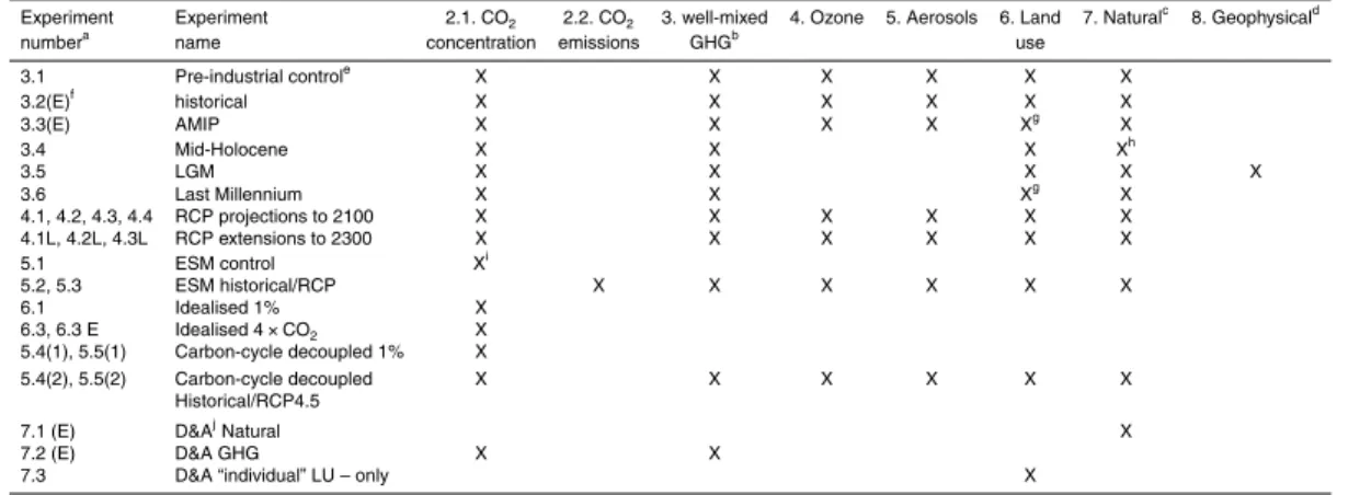
The CMIP5 experiments performed with HadGEM2-ES are listed in Table 1 along with the relevant forcings for each experiment. How these forcings are then imple-mented is detailed in the following sections with Sect. 2 describing the atmospheric

CO2concentrations for the concentration-driven runs as well as the CO2emission

as-15

sumptions for the emission-driven experiments. Section 3 details the boundary condi-tions of atmospheric concentracondi-tions of the other well-mixed greenhouse gases. Tropo-spheric and stratoTropo-spheric ozone assumptions are detailed in Sect. 4. Section 5 details the treatment of aerosols, while Sect. 6 documents that applied to land use pattern changes. Natural forcings, both solar and volcanic, are described in Sect. 7. Apart

20

from these recent history, centennial 21st century and longer-term experiments, we describe as well the setup for the palaeoclimatic runs in Sect. 8. The more general

issue of how the ensemble members are branched offthe control run is described in

Sect. 9, and Sect. 10 concludes. A list of URL locators for websites holding relevant data is included as an Appendix.

(7)

GMDD

4, 689–763, 2011

simulations

C. D. Jones et al.

Title Page

Tables Figures

◭ ◮

Back Close

Full Screen / Esc

Discussion

P

a

per

|

Dis

cussion

P

a

per

|

Discussion

P

a

per

|

Discussio

n

P

a

per

|

2 Carbon dioxide

2.1 CO2concentration

For simulations requiring prescribed atmospheric CO2concentrations, a single global

3-D constant provided as an annual mean mass mixing ratio was used – linearly

in-terpolated in the model at each timestep. This prescribed CO₂ concentration is then

5

passed to the model’s radiation scheme, and constitutes a boundary condition for the

terrestrial and ocean carbon cycle. The oceanic partial pressure of CO2, pCO2, is

always simulated prognostically from this, i.e. it is not itself prescribed.

The CO2 concentrations used were taken from the CMIP5 dataset (see URL 4 in

Appendix A). The historical part of the concentrations (1860–2005) is derived from a

10

combination of the Law Dome ice core (Etheridge et al., 1996), NOAA global mean data (see URL 5 in Appendix A) and measurements from Mauna Loa (Keeling et al., 2009).

After 2005, CO2concentrations recommended for CMIP5 were calculated for the 21st

century from harmonized CO₂emissions of the four IAMs that underlie the four RCPs.

Beyond 2100, these concentrations were extended, so that the CO2concentrations

un-15

der the highest RCP, RCP8.5, stabilize just below 2000 ppm by 2250. Both the medium RCPs smoothly stabilize around 2150, with RCP4.5 stabilizing close to the 2100 value

of the former SRES B1 scenario (∼540 ppm). The lower RCP, RCP3-PD, illustrates a

world with net negative emissions after 2070 and sees declining CO2 concentrations

after 2050, with a decline of 0.5 ppm yr−1 around 2100 (see Fig. 2). These CO₂

con-20

centrations are prescribed in HadGEM2-ES’s historical, AMIP, RCP simulations and the carbon-cycle uncoupled experiments. The detection and attribution experiments

with time varying CO₂ also use these values, but the detection and attribution

exper-iments with fixed CO2 levels use a constant, pre-industrial value of 286.3 ppm. This

CMIP5 dataset also provides the CO2concentration used for the pre-industrial control

25

(8)

GMDD

4, 689–763, 2011

simulations

C. D. Jones et al.

Title Page

Tables Figures

◭ ◮

Back Close

Full Screen / Esc

Discussion

P

a

per

|

Dis

cussion

P

a

per

|

Discussion

P

a

per

|

Discussio

n

P

a

per

|

simulations is described in Sect. 8. More details on the CMIP5 CO₂ concentrations

and how they were derived are provided in Meinshausen et al. (2011).

Aside from these centennial simulations, idealized experiments are performed with HadGEM2-ES for CMIP5 in order to estimate, inter alia, transient and equilibrium cli-mate sensitivity and the clicli-mate-carbon cycle feedback. For the idealised annual 1%

5

increase in CO2concentration, we start from the control-run level of 286.3 ppm in 1859

up to 4×CO₂(1144 ppm) after 140 yr (experiment 6.1). Equivalently, our instantaneous

quadrupling to 4×CO2uses a concentration of 1144 ppm in order to allow diagnosis of

short-term forcing adjustments and equilibrium climate sensitivities (experiment 6.3).

2.1.1 Decoupled carbon cycle experiments 10

Using additional code modifications to the appropriate modules of the HadGEM2-ES

model, it is possible to decouple different carbon-cycle feedbacks. For the decoupled

carbon cycle experiments (5.4, 5.5) we decoupled the climate and carbon cycle in 2 dif-ferent ways. The C4MIP intercomparison exercise (Friedlingstein et al., 2006) defined an “UNCOUPLED” methodology in which only the carbon cycle component responded

15

to changes in atmospheric CO2levels. Gregory et al. (2009) additionally describe the

counterpart experiment where only the model’s radiation scheme responds to changes

in CO₂. Gregory et al. (2009) recommend performing both experiments (as the

re-sults may not combine linearly to give the fully coupled behaviour) and labelling such

experiments in terms of whatisrather thanis notcoupled.

20

Hence we performed the biogeochemically coupled (“BGC”) experiments (5.4) in which the models biogeochemistry is coupled (i.e., the biogeochemistry modules

re-spond to the changing atmospheric CO2 concentration) and the radiation scheme is

uncoupled (and uses the preindustrial level of CO₂ which is held constant) and also

radiatively coupled (“RAD”) experiments (5.5) in which the model’s radiation scheme

25

is allowed to respond to changes in atmospheric CO2 levels, but the biogeochemistry

components (land vegetation and ocean chemistry and ecosystem) use a constant

(9)

GMDD

4, 689–763, 2011

simulations

C. D. Jones et al.

Title Page

Tables Figures

◭ ◮

Back Close

Full Screen / Esc

Discussion

P

a

per

|

Dis

cussion

P

a

per

|

Discussion

P

a

per

|

Discussio

n

P

a

per

|

experiments for the idealised (1%) and transient, multi-forcing (historical/RCP4.5) sce-narios.

2.2 CO₂emissions

2.2.1 Emissions data

In addition to running with prescribed atmospheric CO2concentrations, HadGEM2-ES

5

can be configured to run with a fully interactive carbon cycle. Here, atmospheric CO2

is treated as a 3-D prognostic tracer, transported by atmospheric circulation, and free to evolve in response to prescribed surface emissions and simulated natural fluxes to and from the oceans and land. This approach is required for the “Emission-driven” simulations (5.1–5.3) shown in green text in Fig. 1, and it also allows additional model

10

evaluation by comparison with flask and station measuring sites such as at Mauna Loa (e.g. Law et al., 2006; Cadule et al., 2010).

A 2-D timeseries of total anthropogenic emissions was constructed by summing con-tributions from fossil fuel use and land-use change. For the historical simulation, annual mean emissions from fossil fuel burning, cement manufacture, and gas-flaring were

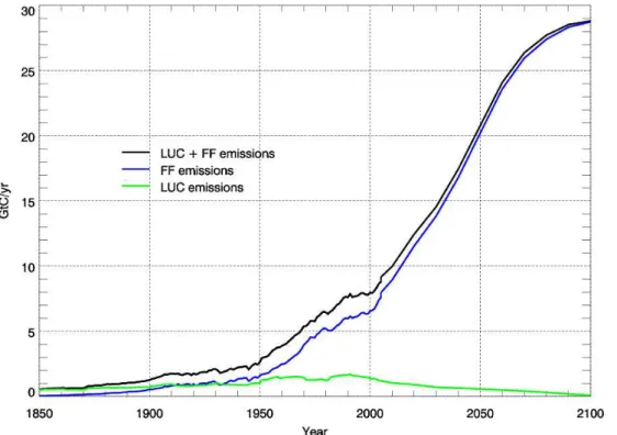
15

provided on a 1◦×1◦grid from 1850 to 1949 (Boden et al., 2010), with monthly means

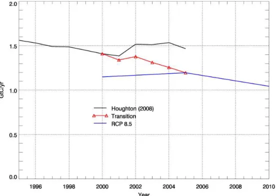
from 1950 to 2005 (Andres et al., 2011). For the RCP8.5 simulation, the harmonized fossil fuel emissions for 2005 to 2100 were used (as available in the RCP database, see URL 6 in Appendix A). The land use change (LUC) emissions are based on the re-gional totals of Houghton (2008), which were provided as annual means of the period

20

1850–2005. Within each of the ten regions the emissions were linearly weighted by

population density on a 1◦×1◦ grid (for more information, see URL 7 in Appendix A).

These population data were also used by Klein Goldewijk (2001) and are linearly in-terpolated between the years 1850, 1900, 1910, 1920, 1930, 1940, 1950, 1960, 1970, 1980, and 1990. After the year 1990 population density is assumed to stay constant.

25

(10)

GMDD

4, 689–763, 2011

simulations

C. D. Jones et al.

Title Page

Tables Figures

◭ ◮

Back Close

Full Screen / Esc

Discussion

P

a

per

|

Dis

cussion

P

a

per

|

Discussion

P

a

per

|

Discussio

n

P

a

per

|

large emissions in urban centres. The weighting with population data inhibits land use change emissions in deserts and high northern latitudes, which improves the

latitudi-nal distribution of the emissions. However, the method is insufficient to provide realistic

local land use change emissions (e.g. in tropical forests).

The gridded (1◦×1◦) fossil fuel and land-use emissions data, originally provided as a

5

flux per gridbox, were converted to flux per unit area, then regridded as annual means onto the HadGEM2-ES model grid. A small scaling adjustment was made after

re-gridding to ensure the global totals matched those of the 1◦×1◦ data exactly. The

CO2 emissions are updated daily in the model by linearly interpolation between the

annual values (or monthly, from 1950 onwards). HadGEM2-ES has the functionality to

10

interactively simulate land-use emissions of CO₂directly from a prescribed scenario of

land-use change and simulated vegetation cover and biomass (see Sect. 6). However, the model has not been fully evaluated in this respect, so for CMIP5 experiments we disable this feature and choose rather to prescribe reconstructed land-use emissions from Houghton (2008). By simulating changes in carbon storage due to imposed land

15

use change, but imposing land-use CO2emissions to the atmosphere from an external

dataset we introduce some degree of inconsistency in this simulation. Work is required to evaluate and improve the simulation of land-use emissions so that they can be used interactively in such simulations in the future.

The uncertainty in annual land-use emissions of±0.5 GtC (cf. Le Qu ´er ´e et al., 2009)

20

is relatively large compared to the total land use emissions (an estimated 1.467 GtC in 2005, Houghton, 2008). The RCP scenarios have been harmonised towards the average LUC emission value of all four original IAM emission estimates, i.e., 1.196 GtC in 2005. This is substantially lower than the value calculated by Houghton (2008) of 1.467 GtC in the same year, although still within the uncertainty. The climate-carbon

25

(11)

GMDD

4, 689–763, 2011

simulations

C. D. Jones et al.

Title Page

Tables Figures

◭ ◮

Back Close

Full Screen / Esc

Discussion

P

a

per

|

Dis

cussion

P

a

per

|

Discussion

P

a

per

|

Discussio

n

P

a

per

|

values were combined in the ratio 80%:20% (Houghton: RCP), followed by 60%:40% in 2002, and so on until 0%:100% (i.e. the RCP value) in 2005, as shown in Fig. 3.

By rescaling the Houghton (2008) data between 2000 and 2005 to merge smoothly with the RCP value in 2005, we lower total emissions in this period by 0.94 GtC com-pared to the original Houghton estimates (Table 2). In the presence of fossil emissions

5

of more than 40 GtC in this period this difference is small. Total emissions and the

relative contribution of fossil fuel and LUC are shown in Fig. 4.

2.2.2 Carbon conservation

In the emissions-driven experiments, conservation of carbon in the earth system is

required. The concentration of atmospheric CO2influences the carbon exchange with

10

the oceans and terrestrial biosphere. Any drift in atmospheric CO₂ will modify these

fluxes accordingly, and thereby impact the land and ocean carbon stores as well as the climate itself. While the transport of atmospheric tracers in HadGEM2-ES is designed to be conservative, the conservation is not perfect and in centennial scale simulations this non-conservation becomes significant. This has been addressed by employing an

15

explicit “mass fixer” which calculates a global scaling of CO2to ensure that the change

in the global mean mass mixing ratio of CO₂ in the atmosphere matches the total flux

of CO₂into or out of it each timestep (Corbin and Law, 2010).

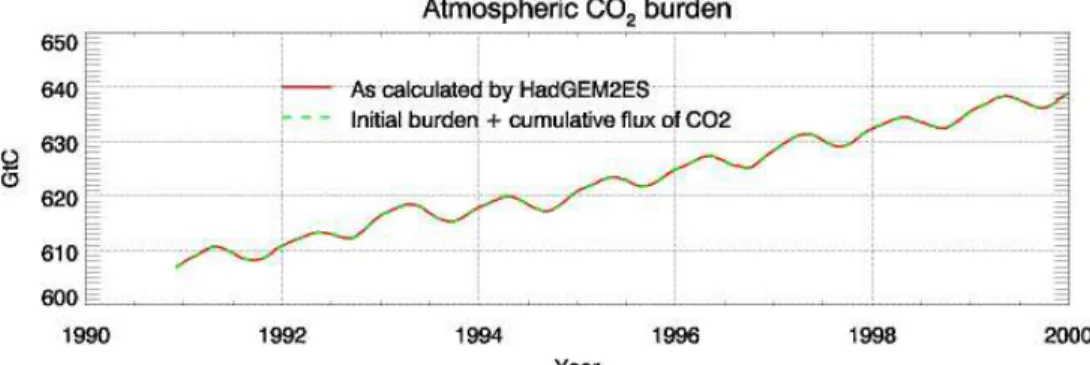
Figure 5 demonstrates HadGEM2-ES’s ability to conserve atmospheric CO2,

follow-ing implementation of the mass fixer scheme described here. The evolution of the

20

atmospheric CO₂burden calculated by the model matches almost exactly the

accumu-lation over time of the CO2flux to the atmosphere. The lower panel of Fig. 5 shows the

difference between the two. This residual difference is most likely explained by changes

in the total mass of the atmosphere in HadGEM2-ES over time, since CO₂mass mixing

ratio is conserved rather than CO2mass. CO2is chemically inert in HadGEM2-ES so

25

(12)

GMDD

4, 689–763, 2011

simulations

C. D. Jones et al.

Title Page

Tables Figures

◭ ◮

Back Close

Full Screen / Esc

Discussion

P

a

per

|

Dis

cussion

P

a

per

|

Discussion

P

a

per

|

Discussio

n

P

a

per

|

3 Non-CO₂well mixed Greenhouse Gases

Specification of the following non-CO2 well-mixed greenhouse gases is required in

HadGEM2-ES: CH₄, N₂O and halocarbons. For the control run, historical and RCP

simulations they are implemented as described below and shown in Fig. 2. The CO2

emissions-driven experiment and the historical/RCP decoupled carbon cycle

experi-5

ments also use these time varying values, as do the AMIP runs and the detection and attribution experiments which require time variation of GHGs. GHG concentrations during the palaeo-climate simulations are described in Sect. 8.

3.1 CH4concentration

Atmospheric methane concentrations were prescribed as global mean mass mixing

10

ratios. For experiments with time-variable CH4 concentrations (historical RCP

ex-periments), these were linearly interpolated from the annual concentrations for every

time step of the model. These interpolated CH₄ concentrations were then passed to

the tropospheric chemistry scheme in HadGEM2-ES (United Kingdom Chemistry and

Aerosols: UKCA, O’Connor et al., 2011). Within UKCA, the surface CH4concentration

15

was forced to follow the prescribed scenario and surface CH4emissions were

decou-pled. CH₄ concentrations above the surface were calculated interactively, and the full

3-D CH4field was then passed from UKCA to the HadGEM2-ES radiation scheme.

As CH4 concentrations were only prescribed at the surface, CH4 in HadGEM2-ES

above the surface is free to evolve in a non-uniform structure and may di_ffer from

pre-20

scribed, well-mixed historical or RCP CH4concentrations. The impact of passing a full

3-D CH4field from UKCA to the radiation scheme rather than passing a uniform

con-centration everywhere was evaluated in a present-day atmosphere-only configuration

of the HadGEM1 model (Johns et al., 2006; Martin et al., 2006). The full 3-D CH4field

lead to the extra-tropical stratosphere being cooler by 0.5–1.0 K, thereby reducing the

25

(13)

GMDD

4, 689–763, 2011

simulations

C. D. Jones et al.

Title Page

Tables Figures

◭ ◮

Back Close

Full Screen / Esc

Discussion

P

a

per

|

Dis

cussion

P

a

per

|

Discussion

P

a

per

|

Discussio

n

P

a

per

|

The CH₄ concentrations used were taken from the recommended CMIP5 dataset.

For the historical period (1860 to 2005), these were assembled from Law Dome ice core measurements reported by Etheridge et al. (1998) and prepared for the NASA GISS model (see URL 8 in Appendix A). Beyond 1984, concentrations were provided by E. Dlugokencky and from the global NOAA/ESRL global monitoring network (see

5

URL 9 in Appendix A). For more details, see Meinshausen et al. (2011). Figure 2b

shows CH₄ concentrations over the historical period (1860 to 2005) and for the RCP

scenarios up to 2300. This dataset also provided the CH4 concentration used in the

pre-industrial control simulation (taken here to be 1860 AD) which was 805.25 ppb.

3.2 N2O concentration

10

Atmospheric N₂O concentrations were prescribed as a time series of annual global

mean mass mixing ratios in the centennial CMIP5 simulations, as described in Mein-shausen et al. (2011). The annual concentrations were linearly interpolated onto the time steps of HadGEM2-ES and passed to the model’s radiation scheme. Figure 2c

shows the N2O concentrations for the 4 RCPs over the historical period and from the

15

RCPs from 2005–2300. This dataset also provided the N2O concentration used in the

pre-industrial control simulation (taken here to be 1860 AD) which was 276.4 ppb.

3.3 Atmospheric halocarbon concentration

Atmospheric concentrations of halocarbons were prescribed as a time series of annual global mean concentrations in the centennial multi-forcing CMIP5 simulations and

in-20

terpolated linearly to the model’s time steps. The future concentrations of halocarbons controlled under the Montreal Protocol are primarily based on the emissions underly-ing the WMO A1 scenario (Daniel et al., 2007) – calculated with a simplified climate model MAGICC, taking into account changes in atmospheric lifetimes due to changes in tropospheric OH-related sinks and stratospheric sinks due to an enhancement of the

25

(14)

GMDD

4, 689–763, 2011

simulations

C. D. Jones et al.

Title Page

Tables Figures

◭ ◮

Back Close

Full Screen / Esc

Discussion

P

a

per

|

Dis

cussion

P

a

per

|

Discussion

P

a

per

|

Discussio

n

P

a

per

|

The CMIP5 dataset provided concentrations of 27 halocarbon species, more than GCMs generally represent separately (for example, HadGEM2-ES explicitly represents the radiative forcing of 6 of these species). The data is therefore also supplied ag-gregated into concentrations of “equivalent CFC-12” and “equivalent HFC-134a”, rep-resenting all gases controlled under the Montreal and Kyoto protocols respectively.

5

These equivalent concentrations were used in HadGEM2-ES (Fig. 2d). Halocarbon concentrations were set to zero for the pre-industrial control run.

The CMIP5 “equivalent” concentrations of CFC12 and HFC134a were derived by simply summing the radiative forcing of individual species and assuming linearity of the relationship between the concentration and radiative forcing for a single species

10

and additivity of multiple species. To quantify the di_fference between using equivalent

CFC-12 and HFC-134a and the full set of possible species a set of five test simulations was completed:

1. Control: halocarbons assumed zero, CO₂at 1×CO₂(286.3 ppm).

2. Halocarbons assumed zero, CO2at 2100 RCP8.5 concentrations (936 ppm).

15

3. Halocarbons assumed constant at 2100 RCP8.5 concentrations (aggregated as

CFC-12eq and HFC-134Aeq), CO₂at 1×CO₂.

4. Halocarbons assumed constant at 2100 RCP8.5 concentrations with Montreal species split (i.e., CFC-11, CFC-12, CFC-113 and HCFC-22, remaining gases

aggregated as CFC-12eq and HFC-134Aeq), CO₂at 1×CO₂.

20

5. Halocarbons assumed constant at RCP8.5 2100 concentrations with Kyoto species split (i.e., HFC-134a and HFC125 and remaining gases aggregated as

CFC-12eq and HFC-134Aeq), CO₂at 1×CO₂.

Upward and downward fluxes of longwave radiation were saved on all vertical levels in the atmosphere after the first model timestep (so that the meteorology is identical).

(15)

GMDD

4, 689–763, 2011

simulations

C. D. Jones et al.

Title Page

Tables Figures

◭ ◮

Back Close

Full Screen / Esc

Discussion

P

a

per

|

Dis

cussion

P

a

per

|

Discussion

P

a

per

|

Discussio

n

P

a

per

|

It should be noted that species not available in HadGEM2-ES are combined into ei-ther HFC-134a or CFC-12 according to their classification. Species are combined into equivalent HFC-134a and CFC-12 by summing their radiative forcing consistently with the CMIP5 methodology. Figure 6 shows excellent agreement between the “equivalent” gases and the more detailed representation from experiments 3, 4, 5 above. Zonal

5

mean differences are within 1 m Wm−2 everywhere showing that the use of 2 CFC

equivalent species in CMIP5 is justified.

4 Ozone

4.1 Tropospheric ozone pre-cursor emissions and concentrations

Tropospheric ozone (O3) is a significant greenhouse gas due to its absorption in the

in-10

frared, visible, and ultraviolet spectral regions (Lacis et al., 1990). It has increased sub-stantially since pre-industrial times, particularly in the northern mid-latitudes (e.g. Stae-helin et al., 2001), which has been linked by various studies to increasing emissions

of tropospheric O3 pre-cursors: nitrogen oxides (NOx=NO+NO2), carbon

monox-ide (CO), methane (CH₄), and non-methane volatile organic compounds (NMVOCs;

15

e.g. Wang and Jacob, 1998). As a result, the tropospheric chemistry configuration of the UKCA model (O’Connor et al., 2011) was implemented in HadGEM2-ES and used

in all CMIP5 simulations to simulate the time evolution of tropospheric O₃interactively

rather than having it prescribed. The UKCA chemistry scheme includes a description

of inorganic odd oxygen (Ox), nitrogen (NOy), hydrogen (HOx), and CO chemistry with

20

near-explicit treatment of CH₄, ethane (C₂H₆), propane (C₃H₈), and acetone (Me₂CO)

degradation (including formaldehyde (HCHO), acetaldehyde (MeCHO), peroxy acetyl nitrate (PAN), and peroxy propionyl nitrate (PPAN). It makes use of 25 tracers and represents 41 species, which participate in 25 photolytic reactions, 83 bimolecular re-actions, and 13 uni- and termolecular reactions. Wet and dry deposition is also taken

25

(16)

GMDD

4, 689–763, 2011

simulations

C. D. Jones et al.

Title Page

Tables Figures

◭ ◮

Back Close

Full Screen / Esc

Discussion

P

a

per

|

Dis

cussion

P

a

per

|

Discussion

P

a

per

|

Discussio

n

P

a

per

|

mean fields and lightning emissions were computed interactively. A full description and evaluation of the chemistry scheme in HadGEM2-ES can be found in O’Connor et al. (2011). Although transport and chemistry were calculated up to the model lid,

boundary conditions were applied within UKCA. In the case of O3, it was

overwrit-ten in those model levels which were 3 levels (approximately 3–4 km) above the

di-5

agnosed tropopause (Hoerling et al., 1993) using the stratospheric O3 concentration

dataset described in Sect. 4.2. It is this combined O3 field which is then passed to

the model’s radiation scheme. Furthermore, oxidation of sulphur dioxide and dimethyl sulphide (DMS) into sulphate aerosol (described in Sect. 5) involves hydroxyl (OH),

hydroperoxyl (HO2), hydrogen peroxide (H2O2), and O3, whose concentrations are

10

provided to the model’s sulphur cycle from UKCA.

No prescribed tropospheric ozone abundance data were used within HadGEM2-ES. Instead, the tropospheric evolution of ozone was simulated using surface and aircraft emissions of tropospheric ozone precursors and reactive gases. It is these emissions, rather than tropospheric ozone concentrations which are held constant in

15

the industrial control simulation. For the palaeoclimate simulations, the same pre-industrial emissions are also used as described in Sect. 8. For the historical and future simulations (including the emissions driven and decoupled carbon cycle experiments, and AMIP runs) a time-varying data set of emissions is used. As the time evolution of tropospheric ozone is simulated rather than prescribed, it may diverge from historical

20

or RCP supplied tropospheric ozone (Lamarque et al., 2011).

The emissions data used by HadGEM2-ES has been supplied for CMIP5 by Lamar-que et al. (2010) and by the IAMs for the 4 RCPs. Speciated surface emissions were provided for the following sectors: land-based anthropogenic sources (agriculture, agri-cultural waste burning, energy production and distribution, industry, residential and

25

(17)

GMDD

4, 689–763, 2011

simulations

C. D. Jones et al.

Title Page

Tables Figures

◭ ◮

Back Close

Full Screen / Esc

Discussion

P

a

per

|

Dis

cussion

P

a

per

|

Discussion

P

a

per

|

Discussio

n

P

a

per

|

burning. This was considered appropriate for biomass burning emissions due to their substantial inter-annual variability both globally and regionally (Lamarque et al., 2010).

All surface emissions were provided as monthly means on a 0.5◦×0.5◦grid. In the case

of aircraft emissions, they were provided as monthly means on a 0.5◦×0.5◦horizontal

grid and on 25 levels in the vertical, extending from the surface up to 15 km.

5

For the UKCA tropospheric chemistry scheme used in HadGEM2-ES, surface

emis-sions for the following species were considered: C2H6, C3H8, CH4, CO, HCHO,

Me₂CO, MeCHO, and NO_x. For the CMIP5 simulations, the spatially uniform surface

CH4concentration is prescribed (as described in Sect. 3.1), and hence the surface CH4

emissions are essentially redundant in this case. For each species the provided

emis-10

sions were re-gridded onto the model’s N96 grid (1.75◦×1.25◦). A small adjustment

was made after re-gridding to ensure the global totals matched those of the original data.

For emissions of C₂H₆, it was decided to combine all C2 species (C₂H₆, ethene

(C2H4), and ethyne (C2H2)) and treat as emissions of C2H6. These were each

con-15

verted to kg(C2H6) m

−2

s−1, added together, and then regridded. For C3H8, the C3

species (propane and propene (C₃H₆)) were similarly combined and treated as

emis-sions of C3H8.

For CO, emissions from land-based anthropogenic sources, biomass burning, and shipping were taken for the historical period from Lamarque et al. (2010). These

20

were added together and re-gridded on to an intermediate 1◦×1◦ grid in terms of

kg(CO) m−2s−1. Oceanic CO emissions were also added (45 Tg(CO) yr−1), and their

spatial and temporal distribution were provided by the Global Emissions Inventory Ac-tivity (see URL 10 in Appendix A), based on distributions of oceanic VOC emissions

from Guenther et al. (1995). In the absence of an isoprene (C5H8) oxidation

mecha-25

nism in the UKCA tropospheric chemistry scheme used in HadGEM2-ES, an additional

354 Tg(CO) yr−1was added based on a global mean CO yield of 30 % from C5H8from

a study by Pfister et al. (2008) and a global C5H8 emission source of 506 TgC yr

−1

(18)

GMDD

4, 689–763, 2011

simulations

C. D. Jones et al.

Title Page

Tables Figures

◭ ◮

Back Close

Full Screen / Esc

Discussion

P

a

per

|

Dis

cussion

P

a

per

|

Discussion

P

a

per

|

Discussio

n

P

a

per

|

from Guenther et al. (1995) and added to the other monthly mean emissions on the

1◦×1◦ grid before regridding.

For HCHO emissions, the monthly mean land-based anthropogenic sources were combined with monthly mean biomass burning emissions from Larmarque et al. (2010a) for the historical period and re-gridded. Similar processing was applied

5

to the future emissions supplied by the IAMs for the 4 RCPs.

For MeCHO, the monthly mean NMVOC biomass burning emissions from

Lamar-que et al. (2010) for the historical period were used. Using different emission

fac-tors from Andreae and Merlet (2001) for grass fires, tropical forest fires, and extra-tropical forest fires, emissions of NMVOCs were converted into emissions of MeCHO

10

(i.e. kg(MeCHO) m−2s−1). Surface emissions of Me₂CO were taken from land-based

anthropogenic sources and biomass burning from Lamarque et al. (2010, 2011). These

were added together and re-gridded on to an intermediate 1◦×1◦ grid in terms of

kg(Me₂CO) m−2s−1. Then, the dominant source of Me₂CO from vegetation was added,

based on a global distribution from Guenther et al. (1995) and scaled to give a global

15

annual total of 40.0 Tg(Me2CO) yr

−1

. The total monthly mean emissions were then re-gridded on to the model’s N96 grid. For future emissions, the processing was identical.

Finally for NOx surface emissions, contributions from land-based anthropogenic

sources, biomass burning, and shipping from Larmarque et al. (2010a) were added

together and re-gridded on to an intermediate 1◦×1◦ grid in terms of kg(NO) m−2s−1.

20

Added to these were a contribution from natural soil emissions, based on a global and

monthly distribution provided by GEIA on a 1◦×1◦ grid (see URL 10 in Appendix A),

and based on the global empirical model of soil-biogenic emissions from Yienger and

Levy II (1995). These were scaled to contribute an additional 12 Tg(NO) yr−1. A similar

approach was adopted when processing the future emissions. All emissions provided

25

were processed as above for the years supplied and a linear interpolation applied be-tween years to produce emissions for every year. Figure 7 shows the time evolution of

tropospheric O3 pre-cursor surface emissions over the 1850–2100 time period. After

(19)

GMDD

4, 689–763, 2011

simulations

C. D. Jones et al.

Title Page

Tables Figures

◭ ◮

Back Close

Full Screen / Esc

Discussion

P

a

per

|

Dis

cussion

P

a

per

|

Discussion

P

a

per

|

Discussio

n

P

a

per

|

In the case of NO_x emissions, 3-D emissions from aircraft were also considered.

These were supplied as monthly mean fields of either NO or NO2 on a 25 level (L25)

0.5×0.5 grid by Lamarque et al. (2010) for the historical period. For HadGEM2-ES

we used the NO emissions. They were first re-gridded on to an N96×L25 grid and

then projected on to the model’s N96×L38 grid, ensuring that the global annual total

5

emissions were conserved. A similar approach was adopted when processing the future emissions.

No additional coding in the HadGEM2-ES or UKCA models was necessary for the treatment of tropospheric ozone pcursor emissions. The only code change was re-quired for the Detection and Attribution “greenhouse gases only” simulation (7.2). In

10

this case, the UKCA model was modified to maintain the global mean surface CH₄

con-centration at pre-industrial levels i.e. 805.25 ppb. This was to ensure that the increase

in CH4concentration as seen by the radiation scheme did not affect concentrations of

tropospheric oxidants, thereby influencing the rate of sulphate aerosol formation.

4.2 Stratospheric ozone concentration 15

HadGEM2-ES requires stratospheric ozone to be input as monthly zonal/height ancil-lary files. CMIP5 recommends the use of the AC&C/SPARC ozone database (Cionni et al., 2011) which covers the period 1850 to 2100 and can be used in climate models that do not include interactive chemistry. The pre-industrial dataset consists of a repeating seasonal cycle of ozone values, and this is also used for the palaeoclimate simulations

20

described in Sect. 8. For the historical and future simulations (including the emissions driven and decoupled carbon cycle experiments, and AMIP runs) a time-varying data set of stratospheric ozone is used.

The historical part of the AC&C/SPARC ozone database spans the period 1850 to 2009 and consists of separate stratospheric and tropospheric data sources. The

fu-25

(20)

GMDD

4, 689–763, 2011

simulations

C. D. Jones et al.

Title Page

Tables Figures

◭ ◮

Back Close

Full Screen / Esc

Discussion

P

a

per

|

Dis

cussion

P

a

per

|

Discussion

P

a

per

|

Discussio

n

P

a

per

|

tropospheric data sources based on 13 CCMs that performed a future simulation until 2100 under the SRES A1B GHG scenario.

The AC&C/SPARC ozone is provided on pressure levels between 1000–1 hPa. The UK National Centre for Atmospheric Science (NCAS) has produced an updated version of the SPARC ozone dataset as follows.

5

A multiple-linear regression was performed on the historical raw pressure-level data between 1000–1 hPa consistent with the Randel and Wu (1999) method

used to construct the timeseries. The ozone was then represented as: O3(t)=

a*SOL+b*EESC+seasonal cycle+residuals. For consistency, the indices of 11-yr

solar cycle (SOL) and total equivalent chlorine (EESC) are identical to those used to

10

prepare the original dataset. The SOL index is a 180.5 nm timeseries provided by Fei Wu at NCAR. The standard SPARC ozone dataset which extends into the future does not include solar cycle variability post-2009. For production of a dataset extending into the future including an 11-yr ozone solar cycle, the solar regression index is used to build a future time series consistent with a repeating solar irradiance compiled by the

15

Met Office Hadley Centre (see Sect. 7.1) and is modelled as a sinusoid with a period

of 11 yr, with mean and max-min values corresponding to solar cycle 23 normalised against the 180.5 nm timeseries used in the historical ozone. There is no solar ozone signal in the high latitudes.

The data were then horizontally interpolated onto a N96 grid. Vertical interpolation

20

was achieved by hydrostatically mapping the SPARC ozone data from pressure sur-faces onto pressure surface equivalent levels corresponding to the height-based grid used by HadGEM2-ES using a scale height of 7 km.

5 Tropospheric aerosol forcing

HadGEM2-ES simulates concentrations of six tropospheric aerosol species:

ammo-25

(21)

GMDD

4, 689–763, 2011

simulations

C. D. Jones et al.

Title Page

Tables Figures

◭ ◮

Back Close

Full Screen / Esc

Discussion

P

a

per

|

Dis

cussion

P

a

per

|

Discussion

P

a

per

|

Discussio

n

P

a

per

|

an ammonium nitrate aerosol scheme is available to HadGEM2-ES, it was still in its de-velopmental version when CMIP5 simulations started, hence nitrate aerosols are not included in the CMIP5 simulations. In addition, secondary organic aerosols from bio-genic emissions are represented by a fixed climatology. All aerosol species can exert

a direct effect by scattering and absorbing shortwave and longwave radiation, and a

5

semi-direct effect whereby this direct effect modifies atmospheric vertical profiles of

temperature and clouds. In HadGEM2-ES all aerosol species, except fossil-fuel black

carbon and mineral dust, also contribute to both the first and second indirect effects

on clouds, modifying cloud albedo and precipitation efficiency, respectively. Changes

in direct and indirect effects since 1860 are termed aerosol radiative forcing. The

10

magnitude of this forcing depends on changes in aerosols, which are due in part to changes in emissions of primary aerosols and aerosol precursors. Changes in emis-sion rates are either derived from external datasets or due to changes in the simulated climate. Here we document how any changes in emission rates are implemented in the HadGEM2-ES CMIP5 centennial experiments. In the control run we specify a

re-15

peating seasonal cycle of 1860 emissions, and this is also used in the palaeoclimate simulations (Sect. 8). Historical and future simulations (including the emissions-driven and decoupled carbon cycle experiments and AMIP runs) use time-varying emissions as described in this section.

In HadGEM2-ES sea-salt and mineral dust aerosol emissions are computed

inter-20

actively, whereas emission datasets drive schemes for sulphate, fossil-fuel black and organic carbon, and biomass aerosols. Unless otherwise stated, datasets are derived from the historical and RCP time series prepared for CMIP5. All non-interactive emis-sion fields are interpolated by the model every five simulated days from prescribed monthly-mean fields. Timeseries of non-interactive emissions are shown in Fig. 10.

25

Aircraft emissions of aerosol precursors and primary aerosols are not included in the model.

The sulphur cycle, which provides concentrations of ammonium sulphate aerosols,

(22)

GMDD

4, 689–763, 2011

simulations

C. D. Jones et al.

Title Page

Tables Figures

◭ ◮

Back Close

Full Screen / Esc

Discussion

P

a

per

|

Dis

cussion

P

a

per

|

Discussion

P

a

per

|

Discussio

n

P

a

per

|

dioxide emissions are derived from sector-based emissions. Emissions for all sec-tors are injected at the surface, except for energy emissions and half of industrial emissions which are injected at 0.5 km to represent chimney-level emissions. Sul-phur dioxide emissions from biomass burning are not included. The model accounts for three-dimensional background emissions of sulphur dioxide from degassing

vol-5

canoes, taken from Andres and Kasgnoc (1998). This represents a constant rate of

0.62 Tg[S] yr−1on a global average, independent of the year simulated and is not part

of the implementation of volcanic climate forcing which we discuss in Sect. 7.2.

Sim-ilarly, land-based DMS emissions do not vary in time and give 0.86 Tg yr−1 (Spiro et

al., 1992). Oceanic DMS emissions are provided interactively by the

biogeochemi-10

cal scheme of the ocean model as a function of local chlorophyll concentrations and mixed layer depth (based on Simo and Dachs, 2002). In an objective assessment against ship-board and time-series DMS observations, the HadGEM2-ES interactive ocean DMS scheme performs with similar skill to that found in the widely used Kettle

et al. (1999) climatology (Halloran et al., 2010). The primary differences between the

15

model-simulated and the climatology-interpolated surface ocean DMS fields are; lower model Southern Hemisphere summer Southern Ocean DMS concentrations, higher model annual equatorial DMS concentrations, and a reduced model seasonal cycle amplitude. Oxidation of sulphur-dioxide and DMS into sulphate aerosol involves

hy-droxyl (OH), hydroperoxyl (HO₂), hydrogen peroxide (H₂O₂), and ozone (O₃):

concen-20

trations for those oxidants are provided by the tropospheric chemistry scheme.

Emissions of primary black and organic carbon from fossil fuel and biofuel are in-jected at 80 m. Emissions of burning aerosols are the sum of the biomass-burning emissions of black and organic carbon. Grassfire emissions are assumed to be located at the surface, while forest fire emissions are injected homogeneously across

25

the boundary layer (0.8 to 2.9 km).

(23)

GMDD

4, 689–763, 2011

simulations

C. D. Jones et al.

Title Page

Tables Figures

◭ ◮

Back Close

Full Screen / Esc

Discussion

P

a

per

|

Dis

cussion

P

a

per

|

Discussion

P

a

per

|

Discussio

n

P

a

per

|

properties. The scheme is described in Woodward (2011). It is based on that designed for HadAM3 (Woodward, 2001) with major developments including the modelling of particles up to 2 mm in the horizontal flux, threshold friction velocities based on Bag-nold (1941), a modified version of the F ´ecan et al. (1999) soil moisture treatment and the utilisation of a preferential source multiplier similar to that described in Ginoux et

5

al. (2001).

Finally, secondary organic aerosols from biogenic emissions are represented by monthly distributions of three-dimensional mass-mixing ratios obtained from a chem-istry transport model (Derwent et al., 2003). These distributions are constant for all simulated years.

10

6 Land-use and land-use change

The HadGEM2-ES land-surface scheme incorporates the TRIFFID DGVM (Cox, 2001), and as such simulates internally the land cover (and its evolution) in response to cli-mate (and clicli-mate change). Hence we do not directly impose prescribed land-cover or vegetation types, but rather provide a fractional mask of anthropogenic disturbance as

15

a boundary condition to the dynamic vegetation scheme. Previous Met Office Hadley

Centre coupled climate-carbon cycle simulations (e.g. Cox et al., 2000; Freidlingstein et al., 2006) used a static (present day) agricultural mask. However the dynamic veg-etation scheme, TRIFFID has now been updated to allow time-varying land-use distri-butions in the CMIP5 simulations.

20

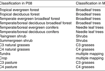
TRIFFID represents the fractional coverage in each grid cell of 5 plant functional types (PFTs: broadleaf tree, needleleaf tree, C3 grass, C4 grass, shrub) and also bare soil. Prescribed fractions of urban areas, lakes and ice are also included from the IGBP land cover map (Loveland et al., 2000) and do not vary in time. The summed fractional coverage of crop and pasture is provided as a time-varying input. Within a

25

(24)

GMDD

4, 689–763, 2011

simulations

C. D. Jones et al.

Title Page

Tables Figures

◭ ◮

Back Close

Full Screen / Esc

Discussion

P

a

per

|

Dis

cussion

P

a

per

|

Discussion

P

a

per

|

Discussio

n

P

a

per

|

trees and shrubs but we do not specify instant replacement by these woody PFTs, but rather their regrowth is simulated by the model’s vegetation dynamics. If woody vegetation cover reduces because of a land use change, vegetation carbon from the removed woody PFTs goes partially to the soil carbon pool and partially to a series of wood products pools. These wood products pools have turnover rates of 1, 10 and

5

100 yr and are not sensitive to environmental conditions. The fraction of vegetation carbon directed into the wood products pool is proportional to the ratio of above ground

and below ground carbon pools ((leaf carbon₊stem carbon)/root carbon). Distribution

of disturbed biomass into the different carbon pools depends on the vegetation type

consistent with McGuire et al. (2008) and is shown in Table 3.

10

HadGEM2-ES is therefore able to simulate both biophysical and biogeochemical ef-fects of land-use change as well as natural changes in vegetation cover in response to

changing climate and CO2. In this version of the model only anthropogenic disturbance

in the form of crop and pasture is represented. Data on within-grid-cell transitions due to shifting cultivation or the impact of wood harvest are not yet used. As described in

15

Sect. 2.2, CO2 emissions from land-use change can be simulated by HadGEM2-ES

but are not used interactively in the emissions driven experiment.

The biophysical impacts of land use change include the direct effect of changes

to surface albedo and roughness due to land-cover change and also changes to the

hydrological cycle due to changes in evapotranspiration and runoff. There is also an

20

indirect physical effect due to changes in surface emissions of mineral dust caused by

changes in bare soil fraction, windspeed and soil moisture, which has a radiative effect

in the atmosphere.

Historic and future simulations (including the emissions-driven and decoupled car-bon cycle simulations and AMIP runs) use time varying disturbance from the Hurtt

25

(25)

GMDD

4, 689–763, 2011

simulations

C. D. Jones et al.

Title Page

Tables Figures

◭ ◮

Back Close

Full Screen / Esc

Discussion

P

a

per

|

Dis

cussion

P

a

per

|

Discussion

P

a

per

|

Discussio

n

P

a

per

|

time varying historical data as in the full historical simulation. For the mid-Holocene

and LGM experiments, there is no agricultural disturbance (which therefore di_ffers from

the control run where a pre-industrial disturbance mask is used). The Last Millennium and AMIP simulations do not use the dynamic vegetation scheme of HadGEM2-ES and instead directly prescribe land-cover as described in Sects. 8 and 9 respectively.

5

The historical land use data is based on the HYDE database v3.1 (Klein Goldewijk et al., 2010, 2011), whilst the future RCP land use scenarios were produced by the respective IAMs and are thus internally consistent with the socio-economic storylines and carbon emissions of the scenarios. A harmonization manipulation was performed, as described in Hurtt et al. (2009, 2010), that attempts to preserve gridded and regional

10

IAM crop and pasture changes as much as possible while minimizing the di_fferences

between the historical estimates and future projections (in 2005). The harmoniza-tion procedure employs the Global Land-use Model (GLM) that ensures a smooth and consistent transition in the harmonization year, grids (or re-grids) the data when nec-essary, spatially allocates national/regional wood harvest statistics, and computes all

15

the resulting land-use states and transitions between land-use states annually from

1500–2100 at half-degree (fractional) spatial resolution, including the effects of wood

harvesting and shifting cultivation. Both historical and future scenarios were made

available at 0.5◦×0.5◦ resolution with annual increments and were downloaded (see

URL 11 in Appendix A).

20

The crop and pasture fraction is re-gridded onto the HadGEM2-ES grid using area average re-gridding. Crop and pasture are then combined to produce a combined “agriculture” mask. It is assumed crop and pasture both mean “only grass, no tree or shrub”. This assumption is simplistic as in some regions of the world “pasture” refers to rangeland where animals are allowed to graze on whatever natural vegetation exists

25

there (which may include trees and shrub). Similarly, woody biofuel crops are treated (erroneously in this case) as non-woody crops. As noted by Hurtt et al. (2010), the

definition and reporting of biofuel differs even within the IAMs producing the 4 RCP

(26)

GMDD

4, 689–763, 2011

simulations

C. D. Jones et al.

Title Page

Tables Figures

◭ ◮

Back Close

Full Screen / Esc

Discussion

P

a

per

|

Dis

cussion

P

a

per

|

Discussion

P

a

per

|

Discussio

n

P

a

per

|

and we expect the impact of any inconsistency to be minor. It remains an outstanding research activity to improve past and present reconstructions of land-cover which can account for temporally and regionally varying changes in definitions and terminology.

An additional uncertainty in reporting the land use carbon fluxes is that the wood products pools are assumed to be zero everywhere at 1860 whilst the terrestrial

car-5

bon cycle (carbon content and vegetation fractions) have been run to equilibrium with 1860 climate and anthropogenic disturbance. Changes in land use cover prior to 1860 involve land use expansion and hence both direct emissions prior to 1860 and some legacy emissions post-1860 due to inputs of disturbed biomass to the soil carbon. No

attempt has been made to include these effects in our output but future work will assess

10

and quantify this e_ffect.

7 Natural climate forcing

HadGEM2-ES can simulate the climate response to two aspects of natural climate forcing: changes in solar irradiance and stratospheric volcanic aerosol. In the control experiment these forcings are kept constant in time. For the historical experiments

(in-15

cluding the emissions-driven and decoupled carbon cycle simulations and AMIP runs) they are varied due to observed reconstructions. For simulations of future periods, where natural forcings are not known, they are varied as described here to minimise the impact of possibly incorrect assumptions about the natural forcings. See Sect. 8 for details on the solar and volcanic forcings applied to the palaeoclimate simulations.

20

7.1 Total solar irradiance

The way the model deals with variations in total solar irradiance (TSI) is the same as in earlier generations of Hadley Centre models, HadCM3 (Stott et al., 2000, Tett et al., 2002) and HadGEM1 (Stott et al., 2006). Annual mean variations in TSI are parti-tioned across the six shortwave spectral bands (0.2–10 µm) to estimate the associated