Annales
Geophysicae
Geomagnetic storm effects at F1-layer heights from incoherent
scatter observations
A. V. Mikhailov1and K. Schlegel2
1Institute of Terrestrial Magnetism, Ionosphere and Radio Wave Propagation, Troitsk, Moscow Region 142190, Russia 2Max-Planck-Institute f¨ur Aeronomie, Max-Planck-Str. 2, D-37191 Katlenburg-Lindau, Germany
Received: 18 April 2002 – Revised: 24 July 2002 – Accepted: 30 August 2002
Abstract. Storm effects at F1-layer heights (160–200 km) were analyzed for the first time using Millstone Hill (mid-latitudes) and EISCAT (auroral zone) incoherent scatter (IS) observations. The morphological study has shown both in-creases (positive effect) and dein-creases (negative effect) in electron concentration. Negative storm effects prevail for all seasons and show a larger magnitude than positive ones, the magnitude of the effect normally increasing with height. At Millstone Hill the summer storm effects are small compared to other seasons, but they are well detectable. At EISCAT this summer decrease takes place only with respect to the au-tumnal period and the autumn/spring asymmetry in the storm effects is well pronounced. Direct and significant correla-tion exists between deviacorrela-tions in electron concentracorrela-tion at the F1-layer heights and in the F2-layer maximum. Unlike the F2-layer the F1-region demonstrates a relatively small reaction to geomagnetic disturbances despite large pertur-bations in thermospheric parameters. Aeronomic parame-ters extracted from IS observations are used to explain the revealed morphology. A competition between atomic and molecular ion contributions toN evariations was found to be the main physical mechanism controlling the F1-layer storm effect. The revealed morphology is shown to be related with neutral composition (O, O2, N2) seasonal and storm-time variations. The present day understanding of the F1-region formation mechanisms is sufficient to explain the observed storm effects.
Key words. Atmospheric composition and structure (thermosphere-composition and chemistry); ionosphere (ion chemistry and composition; ionospheric disturbances)
1 Introduction
Ionospheric disturbances related to geomagnetic storms are widely discussed in literature (see the reviews by Pr¨olss,
Correspondence to:K. Schlegel ([email protected])
1995; Buonsanto, 1999; Mikhailov, 2000; Richmond, 2000; Danilov and Lastovicka, 2001 and references therein). The main attention is paid to the F2-layer storm effects being the most pronounced and impressive, while F1-layer distur-bances are practically not discussed. On the one hand, this is due to the problems with thefoF1 identification (Shchepkin and Vinitzky, 1981); on the other hand, F1-layer storm ef-fects are relatively small compared to the F2-layer ones and are not very important from the radio-wave propagation point of view. Theory of the F1-layer formation (Shchepkin, 1969; Shchepkin et al., 1972; Antonova and Ivanov-Kholodny, 1988a, b) indicates a close relationship between F1-layer electron concentration and neutral composition. Therefore, the observed small reaction of the F1-region to the geomag-netic disturbances followed by large perturbations in the ther-mospheric parameters is interesting from a physical point of view and should be explained. Recently, Buresova and Las-tovicka (2001), and Buresova et al. (2002) have attempted to systematize the F1-layer storm effects analyzingN e(h) pro-files obtained from the ionogram reduction over some Eu-ropean ionosonde stations. The analysis revealed two in-teresting effects: (i) independently of the sign of the F2-layer disturbance (positive or negative), the F1-F2-layer elec-tron concentration always decreases (negative storm effect), (ii) there exists a summer/winter and autumn/spring asym-metry in the F1-layer geomagnetic storm effects. They have shown that the summer F1-layer (the electron concentration at 160–190 km) practically does not react to geomagnetic storms, while a well detectable negative storm effect takes place in winter, and also, that autumnal storm effects are stronger than vernal ones. These conclusions need further analysis to check whether such an F1-layer reaction is sys-tematic or the results just reflect the peculiarity of the ob-servations chosen. Electron concentration both in the F2-and F1-regions is known to be strongly dependent on neu-tral composition as the processes of photoionization and re-combination are mainly the same. So, in principle, one may expect a synchronous (to some extent) type of NmF2 and
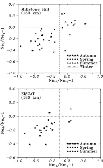
Fig. 1.The relative (disturbed/quiet) deviationsδN eat 180 km ver-sus relative deviationsδN mF2 for Millstone Hill and EISCAT storm observations.
seem to confirm this. With respect to the sign of the F1-layer storm effect, the ionogram reduction for Moscow (Zevakina et al., 1971) yielded in some cases positive1N eat F1-layer heights during daytime hours. Therefore, the aim of the pa-per is to analyze the effects of geomagnetic disturbances at F1-layer heights (160–200 km) using Millstone Hill (middle latitudes) and EISCAT (auroral zone) incoherent scatter (IS) daytime observations, and to give a physical interpretation to the revealedN e(h) variations.
2 Observations
All available Millstone Hill (zenith observations) and EIS-CAT CP-1 and CP-2 (field-aligned multi-pulse, as well as long-pulse) observations were examined to select couples (disturbed/reference) of days with daytime observations. We have tried to choose reference days to be geomagnetically quiet and close in time to the analyzed disturbed ones, but this was impossible in some cases due to irregular
observa-tions. Usually Millstone Hill radar provides three (some-times more) local height N e, T e, T i and V z profiles per hour, with a 21-km height resolution. We had to use a 3– 4 h period of observation to calculate median height profiles with the standard deviations (SD) at each height. These me-dian profiles were then smoothed by a polynomial fit up to the 5th order to be used in our analysis.
EISCAT multi-pulse observations provide excellent height profiles with a 3-km height resolution in the 87–260 km height range. Due to frequent (every 2–5 min) observations, median profiles can be calculated over a 1–2 h period; there-fore, for the interesting cases, two different periods within one day can be considered for analysis (24/25 October 1990). Usually the periods around noon of maximal stability in
NmF2 and hmF2 variations were selected to decrease the scatter and provide reliable medianN e(h) profiles. Unlike Millstone Hill the EISCATN e(h) profiles are not normalized byfoF2 for each particular experiment, and this may result in wrong relative deviations when disturbed and reference days are compared. Therefore, the following procedure was ap-plied. Long-pulse observations are known to provide reliable relativeN e(h) profiles at the F2-region heights. Using the long-pulseNmF2/N e(220 km) ratio, the multi-pulseNmF2 value was calculated assuming that relativeN e(h) height pro-files are the same in the (220 km –hmF2) height range both for long-pulse and multi-pulse observations. This calculated
NmF2 was then normalized by the observedfoF2 value mea-sured by the Tromsø or Kiruna ionosondes. Then the whole N e(h)multi-pulse profile was normalized by a correspond-ing factor.
The observations were grouped by 4 seasons regardless of the solar activity level. Since we analyzed only sunlit conditions EISCAT winter observations were not included. The list of analyzed dates (disturbed/reference), along with daily Ap and F10.7 indices, are given in Tables 1 and 2 for Millstone Hill and EISCAT, correspondingly. The ratios r = Ndist/Nref, along with absolute errors forNmF2 and N eat 5 heights (160–200 km), are given in the tables. Over-all, 37 cases from Millstone Hill and 26 cases from EISCAT were analyzed. The observations are seen to overlap all lev-els of solar activity from the deep minima in 1986, 1996 to the maximum in 1990–1991. A strong scatter in observa-tions for some dates (especially at Millstone Hill) results in abnormal SD values, and such cases are marked by dashes in Tables 1 and 2. With regard to this, it should be noted that while some wrong (due to occasional scatter)N evalues may strongly affect the calculated SD, the median values used in our analysis are much less sensitive to such scatter and are more reliable compared to meanN evalues.
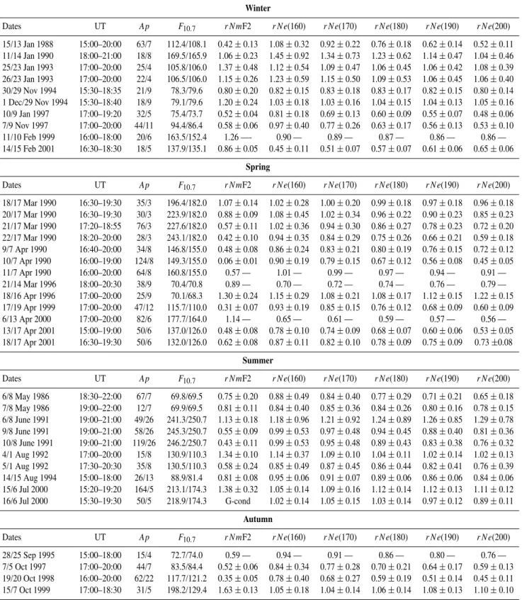
Table 1. List of Millstone Hill observations (disturbed/reference days), together with dailyApandF10.7indices. ObservedrN mF2 and
rN eat 160–200 km heights are given, together with absolute deviations (dashes correspond to large scatter in data when calculated standard deviations are unreliable). G-conditions means the absence of the F2-layer peak, LT=UT-5
Winter
Dates UT Ap F10.7 rNmF2 rNe(160) rNe(170) rNe(180) rNe(190) rNe(200)
15/13 Jan 1988 15:00–20:00 63/7 112.4/108.1 0.42±0.13 1.08±0.32 0.92±0.22 0.76±0.18 0.62±0.14 0.52±0.11 11/14 Jan 1990 18:00–21:00 18/8 169.5/165.9 1.06±0.23 1.45±0.92 1.34±0.73 1.23±0.62 1.14±0.47 1.04±0.46 25/23 Jan 1993 17:00–20:00 25/4 105.8/106.0 1.37±0.48 1.12±0.54 1.09±0.47 1.06±0.45 1.06±0.42 1.08±0.39 26/23 Jan 1993 17:00–20:00 22/4 106.5/106.0 1.15±0.26 1.23±0.59 1.15±0.50 1.09±0.53 1.06±0.45 1.06±0.40 30/29 Nov 1994 15:30–18:35 21/9 78.3/79.6 0.80±0.20 0.82±0.15 0.83±0.18 0.83±0.17 0.82±0.15 0.80±0.14 1 Dec/29 Nov 1994 15:30–18:40 18/9 79.1/79.6 1.20±0.24 1.03±0.18 1.03±0.16 1.04±0.15 1.04±0.13 1.05±0.16 10/9 Jan 1997 17:00–19:20 32/5 75.4/73.7 0.52±0.04 0.81±0.18 0.69±0.13 0.60±0.09 0.55±0.07 0.48±0.06 7/9 Nov 1997 17:00–20:00 44/11 94.4/86.4 0.58±0.06 0.97±0.40 0.77±0.26 0.63±0.17 0.56±0.13 0.53±0.10 11/10 Feb 1999 16:00–18:00 20/6 163.5/152.4 1.26 —- 0.90 — 0.89 — 0.87 — 0.86 — 0.86 — 14/15 Feb 2001 16:30–18:30 18/5 137.9/135.1 0.86±0.05 0.45±0.11 0.51±0.07 0.57±0.07 0.61±0.06 0.65±0.06
Spring
Dates UT Ap F10.7 rNmF2 rNe(160) rNe(170) rNe(180) rNe(190) rNe(200)
18/17 Mar 1990 16:30–19:30 35/3 196.4/182.0 1.07±0.14 1.02±0.28 1.00±0.20 0.99±0.18 0.97±0.18 0.96±0.18 20/17 Mar 1990 16:30–19:30 30/3 223.9/182.0 0.88±0.09 1.08±0.45 1.02±0.34 0.96±0.22 0.90±0.23 0.85±0.23 21/17 Mar 1990 17:20–18:55 76/3 227.6/182.0 0.57±0.11 1.02±0.36 0.94±0.30 0.86±0.27 0.78±0.23 0.72±0.20 22/17 Mar 1990 18:20–20:00 28/3 243.1/182.0 0.42±0.10 0.94±0.35 0.84±0.29 0.75±0.26 0.66±0.21 0.59±0.18 9/7 Apr 1990 16:40–20:00 34/8 146.8/155.0 0.48±0.08 0.86±0.24 0.83±0.21 0.80±0.19 0.76±0.15 0.72±0.12 10/7 Apr 1990 16:00–19:00 124/8 149.3/155.0 0.06±0.01 0.90±0.19 0.79±0.15 0.67±0.12 0.56±0.08 0.45±0.05 11/7 Apr 1990 16:00–20:00 64/8 160.8/155.0 0.57 — 1.01 — 0.99 — 0.97 — 0.94 — 0.91 — 21/14 Mar 1996 18:00–20:30 38/9 70.4/70.8 0.89 — 0.70 — 0.72 — 0.74 — 0.76 — 0.79 — 18/16 Apr 1996 17:00–20:00 25/9 70.1/68.3 1.30±0.24 1.15±0.29 1.08±0.21 1.08±0.17 1.12±0.15 1.22±0.15 17/19 Apr 1999 17:00–20:00 47/12 115.7/110.0 0.31±0.07 0.93±0.19 0.85±0.15 0.76±0.12 0.68±0.09 0.60±0.09 6/13 Apr 2000 17:00–20:00 82/6 177.7/164.0 1.14 — 0.65 — 0.61 — 0.59 — 0.57 — 0.56 — 13/17 Apr 2001 15:00–19:00 50/6 137.0/126.0 0.48±0.08 0.78±0.10 0.74±0.09 0.68±0.07 0.60±0.06 0.53±0.05 18/17 Apr 2001 16:30–19:30 50/6 132.0/126.0 0.62±0.08 0.87±0.11 0.82±0.10 0.78±0.09 0.75±0.09 0.73±0.08
Summer
Dates UT Ap F10.7 rNmF2 rNe(160) rNe(170) rNe(180) rNe(190) rNe(200)
6/8 May 1986 18:30–22:00 67/7 69.8/69.5 0.75±0.20 0.88±0.49 0.84±0.40 0.77±0.29 0.71±0.21 0.65±0.18 7/8 May 1986 19:00–22:00 12/7 69.9/69.5 0.81±0.11 0.84±0.40 0.85±0.36 0.84±0.26 0.80±0.16 0.78±0.15 6/8 June 1991 19:00–21:00 49/26 241.3/250.7 1.13±0.18 1.18±0.96 1.21±0.92 1.24±0.89 1.26±0.85 1.29±0.78 9/8 June 1991 19:00–21:00 58/26 245.3/250.7 0.55±0.09 0.99±0.53 0.97±0.48 0.94±0.45 0.88±0.40 0.81±0.36 10/8 June 1991 19:00–21:00 119/26 246.2/250.7 0.43±0.11 0.99±0.53 0.95±0.48 0.89±0.43 0.83±0.38 0.76±0.32 4/1 Aug 1992 17:00–20:00 15/8 130.9/110.3 1.34±0.10 1.14±0.37 1.09±0.10 1.04±0.11 1.02±0.14 1.02±0.13 5/1 Aug 1992 17:30–20:30 35/8 130.5/110.3 0.58±0.24 0.85±0.49 0.87±0.45 0.86±0.44 0.82±0.41 0.76±0.39 14/15 Aug 1994 15:00–18:00 26/13 88.9/81.4 0.81±0.08 0.95±0.06 0.91±0.07 0.89±0.06 0.86±0.06 0.84±0.06 15/6 Jul 2000 15:20–19:20 164/5 213.1/174.3 1.38±0.32 1.05±0.14 1.09±0.16 1.12±0.14 1.12±0.13 1.11±0.12 16/6 Jul 2000 15:30–19:30 50/5 218.9/174.3 G-cond 1.02±0.14 1.05±0.15 1.03±0.14 0.97±0.12 0.89±0.11
Autumn
Dates UT Ap F10.7 rNmF2 rNe(160) rNe(170) rNe(180) rNe(190) rNe(200)
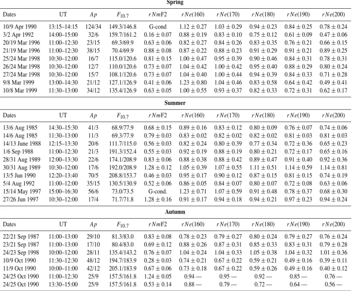
Table 2. List of EISCAT observations (disturbed/reference days), together with dailyAp andF10.7indices. ObservedrN mF2 andrN e at 160–200 km heights are given, together with absolute deviations (dashes correspond to large scatter in data when calculated standard deviations are unreliable). G-conditions means the absence of the F2-layer peak, LT=UT+1
Spring
Dates UT Ap F10.7 rNmF2 rNe(160) rNe(170) rNe(180) rNe(190) rNe(200)
10/9 Apr 1990 13:15–14:15 124/34 149.3/146.8 G-cond 1.12±0.27 1.03±0.29 0.94±0.23 0.84±0.25 0.78±0.24 3/2 Apr 1992 14:00–15:00 32/6 159.7/161.2 0.16±0.07 0.88±0.19 0.83±0.10 0.75±0.12 0.61±0.09 0.47±0.06 20/19 Mar 1996 11:00–12:30 23/15 69.3/69.9 0.63±0.06 0.82±0.27 0.84±0.26 0.83±0.35 0.76±0.21 0.66±0.15 21/19 Mar 1996 11:00–12:30 38/15 70.4/69.9 0.88±0.08 0.87±0.22 0.88±0.23 0.91±0.29 0.91±0.21 0.89±0.25 25/24 Mar 1998 10:30–12:00 16/7 115.0/120.6 0.81±0.15 1.00±0.47 0.95±0.39 0.90±0.46 0.84±0.31 0.78±0.31 26/24 Mar 1998 10:30–12:00 12/7 110.0/120.6 0.73±0.07 1.04±0.42 1.00±0.42 0.95±0.40 0.88±0.29 0.80±0.24 27/24 Mar 1998 10:30–12:00 15/7 108.1/120.6 0.73±0.07 1.04±0.40 1.00±0.44 0.94±0.39 0.84±0.33 0.71±0.28 9/8 Mar 1999 13:00–14:30 21/12 127.1/126.9 0.41±0.06 1.23±0.80 1.04±0.46 0.83±0.58 0.64±0.42 0.49±0.41 10/8 Mar 1999 11:30–13:00 34/12 135.4/126.9 0.63±0.05 1.00±0.55 0.93±0.37 0.82±0.33 0.72±0.31 0.62±0.17
Summer
Dates UT Ap F10.7 rNmF2 rNe(160) rNe(170) rNe(180) rNe(190) rNe(200)
13/6 Aug 1985 14:30–15:30 41/3 68.9/77.9 0.68±0.15 0.89±0.16 0.83±0.12 0.80±0.09 0.76±0.07 0.74±0.06 14/6 Aug 1985 11:30–13:00 11/3 69.3/77.9 0.79±0.03 0.83±0.02 0.82±0.02 0.82±0.02 0.81±0.03 0.81±0.03 14/13 June 1988 12:15–13:30 20/6 111.7/115.0 0.56±0.03 0.82±0.24 0.80±0.39 0.77±0.34 0.72±0.36 0.65±0.23 1/6 Sep 1988 11:00–12:30 21/3 191.3/152.4 0.55±0.03 0.92±0.19 0.88±0.19 0.80±0.21 0.72±0.17 0.65±0.16 28/31 Aug 1989 12:00–13:30 22/6 174.1/208.9 0.83±0.06 0.88±0.38 0.88±0.42 0.89±0.47 0.91±0.40 0.92±0.36 30/31 Aug 1989 10:30–12:00 17/6 192.0/208.9 1.28±0.12 1.05±0.39 1.07±0.55 1.11±0.51 1.14±0.59 1.14±0.81 13/5 Jun 1990 12:20–13:40 70/5 208.8/153.7 0.46±0.03 0.95±0.17 0.90±0.12 0.87±0.15 0.81±0.15 0.74±0.19 5/4 Aug 1992 11:00–12:00 35/15 130.5/130.9 0.52±0.06 0.86±0.05 0.84±0.07 0.80±0.07 0.72±0.08 0.63±0.06 15/14 May 1997 15:00–16:30 56/6 73.0/73.5 G-cond. 1.23±0.71 1.07±0.59 0.91±0.48 0.78±0.37 0.68±0.30 27/26 Jun 1997 10:30–12:00 17/4 71.7/71.8 1.28±0.16 0.91±0.17 0.94±0.18 0.94±0.21 0.97±0.23 0.94±0.24
Autumn
Dates UT Ap F10.7 rNmF2 rNe(160) rNe(170) rNe(180) rNe(190) rNe(200)
22/21 Sep 1987 11:00–13:00 29/10 81.3/83.0 0.83±0.08 0.78±0.23 0.79±0.27 0.80±0.24 0.79±0.27 0.76±0.24 23/21 Sep 1987 11:00–13:00 17/10 80.4/83.0 0.69±0.12 0.88±0.26 0.87±0.31 0.85±0.33 0.83±0.31 0.79±0.28 24/23 Sep 1998 10:00–12:00 28/11 135.4/143.2 0.76±0.07 1.04±0.24 1.04±0.33 1.05±0.38 1.04±0.32 1.01±0.36 10/9 Oct 1990 11:30–12:30 48/12 194.7/183.9 0.28±0.03 0.74±0.21 0.67±0.22 0.59±0.21 0.49±0.16 0.39±0.11 11/9 Oct 1990 10:00–11:00 42/12 205.1/183.9 0.67±0.06 0.73±0.18 0.67±0.22 0.59±0.26 0.49±0.16 0.40±0.12 24/25 Oct 1990 11:00–12:30 25/9 157.5/161.8 1.24±0.05 0.94 — 0.95 — 0.92 — 0.85 — 0.76 — 24/25 Oct 1990 13:30–15:00 25/9 157.5/161.8 0.53±0.14 0.88 — 0.79 — 0.72 — 0.64 — 0.56 —
only slightly disturbed (e.g. 9 April 1990, 4 August 1992 from Table 2). The choice of 8 June 1991 and 20 October 1998 (Table 1) as the reference days is due to the absence of available quiet days nearby.
3 Data analysis
Millstone Hill observations (Table 1) show both negative and positive storm effects for all seasons, but negative deviations prevail. As a rule, positive deviations are relatively small compared to negative ones. At EISCAT (the auroral zone) negative deviations dominate (Table 2). Some cases of small positive storm effects (30/31 August 1989, 24/23 September 1998) may be related to uncertainties offoF2 readings from ionograms used for theN e(h) profile normalization. On the other hand, positive deviations are more pronounced at lower
heights (160 km), and this may be due to particle precipita-tion effects during disturbed periods.
Usually the amplitude of deviation increases with height (a decrease inrN ein Tables 1 and 2), especially for negative storm effect, but the inverse type of dependence is possible as well (26/23 January 1993, 11/14 January 1990; 14/15 Febru-ary 2001; 4/1 August 1992 from Table 1 or 21/19 March 1996, 28/31 August 1989 from Table 2).
For the convenience of presentation we will consider δN e = rN e − 1, together with rN e. Figure 1 shows theδN e (at 180 km) versusδN mF2 = (NmF2dist –
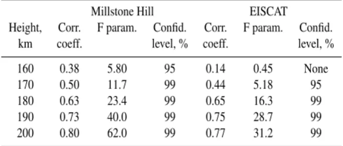
sea-Table 3.Correlation betweenδN eat F1-layer heights andδN mF2 for Millstone Hill and EISCAT
Millstone Hill EISCAT
Height, Corr. F param. Confid. Corr. F param. Confid.
km coeff. level, % coeff. level, %
160 0.38 5.80 95 0.14 0.45 None
170 0.50 11.7 99 0.44 5.18 95
180 0.63 23.4 99 0.65 16.3 99
190 0.73 40.0 99 0.75 28.7 99
200 0.80 62.0 99 0.77 31.2 99
sons from Tables 1 and 2 and calculated the correlation co-efficients betweenδN e(180) andδN mF2. The test of sta-tistical significance for this correlation was made with the Fisher’s F-criterion (Pollard, 1977). The results are given in Table 3. The correlation coefficients are seen to be not very large but they are significant at the 95–99% confidence level. The observations at 160 km show large scatter and look less reliable compared to higher altitudes.
The results by Buresova and Lastovicka (2001) and Buresova et al. (2002) show some seasonal effect (win-ter/summer and autumn/spring asymmetry) in theNeF1 re-action to the geomagnetic disturbances. We have calculated averagerN efrom Tables 1 and 2 for different seasons. These average values, along with the standard deviations, are given in Table 4 for Millstone Hill and EISCAT. The storm ef-fect is seen to be less in summer compared to other seasons at Millstone Hill. At EISCAT this summer effect is seen only with respect to autumn, but an autumn/spring asymme-try is clearly present in the storm effect. To check whether these seasonal differences are significant, we put together all heights in Table 4 and applied the Student’s T-criterion (Pollard, 1977), which examines whether the difference be-tween two average values is significant. At Millstone Hill the summer/winter difference is significant at the 90%, sum-mer/spring – at 99.9%, summer/autumn – at 99.9% confi-dence level, while the autumn/spring difference is insignif-icant. At EISCAT the summer/autumn difference is signifi-cant at the 99%, autumn/spring – at 97.5% confidence level, while the summer/spring difference is insignificant. Table 4 also shows the decrease with height in calculatedrN e, in-dicating the increase in the storm effect with height for all seasons.
The results of the morphological analysis may be summa-rized as follows:
1. The storm effects may be positive and negative but neg-ative deviations prevail. As a rule, positive storm effects are small compared to negative ones.
2. Usually the amplitude of the storm effect increases with height (especially for negative ones), but cases with the inverse type of dependence also take place both at Mill-stone Hill and EISCAT.
3. There is a direct and significant correlation between δN eat F1-layer heights andδN mF2, the correlation co-efficients increasing with height.
4. At Millstone Hill the summer storm effects inδN eare less compared to other seasons, but they are well de-tectable, nevertheless. At EISCAT an autumn/spring asymmetry in the storm effect is well pronounced, while the summer effect takes place only with respect to the autumnal season. These differences are statistically sig-nificant.
5. It should be stressed that in general a relatively small sensitivity of the F1-region to geomagnetic disturbances exists despite large storm perturbations in the thermo-spheric parameters (see later). This is quite different from the F2-layer storm behavior.
An interpretation of the revealed morphological features is given below based on the contemporary understanding of the ionosphere formation at F1-layer heights.
4 Model calculations
To understand the physical mechanism of the revealed F1-layer storm effects, one should consider the aeronomic pa-rameters responsible for the F1-layer formation during quiet and disturbed conditions. A method proposed by Mikhailov and Schlegel (1997), with later modifications (Mikhailov and F¨orster, 1999; Mikhailov and Schlegel, 2000) applied earlier to Millstone Hill observations (Mikhailov and Fos-ter, 1997; Mikhailov and F¨orsFos-ter, 1997, 1999) and EIS-CAT observations (Mikhailov and Schlegel, 1998; Mikhailov and Kofman, 2001) is used here. It allows us to find in a self-consistent way neutral composition (O, O2, N2 concen-trations), neutral temperature specified by three parameters (Tex, T120, S), total EUV solar flux withλ < 1050 ˚A, and ion composition. Vertical plasma drift related to thermo-spheric winds and electric fields can also be derived with this method, but they are not used in the present analysis. The details of the method may be found in the above refer-ences; therefore, only the main idea is sketched here. The model used includes: transport process for O+(4S)and pho-tochemical processes only for O+(2D), O+(2P), O+2(X2Q), N+,N+
2 and NO+ions in the 120–550 km height range. De-pending on conditions the height interval can be changed (for instance, to avoid the precipitation effect at lower heights) and the observed electron concentration is used as the bound-ary condition. A two-component model of the solar EUV from Nusinov (1992) is used to calculate the photoionization rates in 35-wavelength intervals (100–1050 ˚A). The photo-ionization and photo-absorption cross sections are obtained from Torr et al. (1979) and Richards and Torr (1988). Flow-ing afterglow laboratory measurements of the O++N
Table 4.Observed seasonal variation of therN evalues at F1-layer heights for Millstone Hill and EISCAT. Average daytime values along with standard deviations are given
Height Millstone Hill EISCAT
km Winter Spring Summer Autumn Spring Summer Autumn
160 0.99±0.27 0.92±0.15 0.99±0.12 0.90±0.12 1.00±0.13 0.93±0.12 0.86±0.11 170 0.92±0.24 0.86±0.14 0.98±0.12 0.85±0.16 0.94±0.08 0.90±0.10 0.83±0.14 180 0.87±0.23 0.82±0.14 0.96±0.14 0.80±0.20 0.87±0.07 0.87±0.10 0.79±0.17 190 0.83±0.23 0.77±0.17 0.93±0.17 0.76±0.24 0.78±0.11 0.83±0.13 0.73±0.20 200 0.81±0.25 0.74±0.21 0.89±0.19 0.72±0.28 0.69±0.14 0.79±0.16 0.67±0.23
difference between measured total vertical plasma velocity and diffusion velocity for O+ ions. Collisions of O+ ions with neutral O, O2, N2and NO+, O+2, N+2, N+ions are taken into account. All O+ion collision frequencies are taken from Banks and Kockarts (1973). Ion concentrations are known at each iteration step from fitting calculatedN e(h)to the exper-imental ones. Using standard multi-regressional methods we fit the calculatedN e(h)profile to the observed one and find the earlier mentioned aeronomic parameters. The estimated accuracy of the extracted thermospheric parameters is about ±20–25% (Mikhailov and Schlegel, 1997, 2000).
Four cases (disturbed/quiet) of days presenting different seasons were analyzed. Winter and spring are presented by Millstone Hill observations on 7/9 November 1997 and 22/17 March 1990, with a well pronounced negative storm effect and increasingδN e with height. Summer and autumn are presented by EISCAT observations on 13/5 June 1990 and 1/6 September 1988, with small storm effects at F1-layer heights. In fact, the 1/6 September case may be prescribed to summer and later, we will refer to June 1990 and Septem-ber 1988 periods as “summer”. Since winter and equinoctial periods demonstrate similar storm effects (Table 4), we will refer to November 1997 and March 1990 periods as “winter” in further discussion.
Millstone Hill observations during a very severe geomag-netic storm on 15–16 July 2000 were also analyzed. This period considered by Buresova et al. (2002) is distinguished by small F1-layer storm effects, despite the extremely strong geomagnetic storm withApindex up to 164.
The selected EISCAT observations are characterized by small (E < 7 mV/m) electric fields in order not to intro-duce additional effects (St.-Maurice and Schunk, 1979; Hu-bert and Kinzelin, 1992) to the model calculations. This al-lows us to consider the daytime auroral ionosphere as a mid-latitude one (Farmer et al., 1984; Lathuilli`ere and Brekke, 1985). However, EISCAT is located in the auroral zone, and particle precipitation takes place in some cases during dis-turbed periods. For instance, 25 September 1998 was not used in our analysis for this reason; a pronounced increase in Ne obviously related with particle precipitation took place at lower heights on 9 March 1999. But such cases are not numerous in our analysis.
The experimentalN e(h),T e(h),T i(h)profiles were cor-rected for disturbed days when the calculated ion
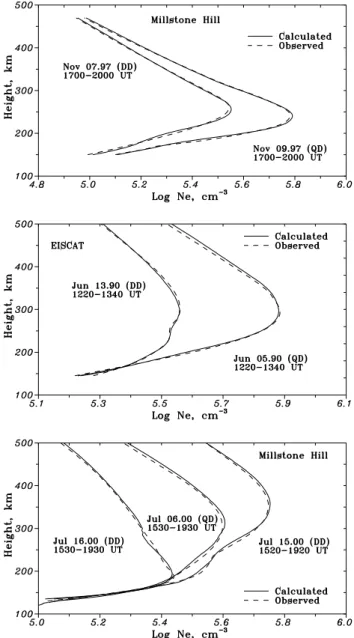
composi-Fig. 2. Observed (corrected on ion composition) and calculated
N e(h)profiles for winter (7/9 November 1997), summer (13/5 June 1990) and a very severe geomagnetic storm on 15–16 July 2000.
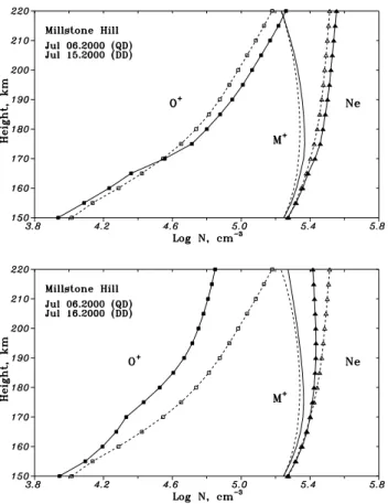
Fig. 3.Calculated distribution of atomic oxygen O+and molecular M+ions as well as their sum, Ne for winter (7 Nov/9 Nov 1997) and summer (13 Jun/5 Jun 1990) disturbances. Solid lines and filled symbols refer to the disturbed days.
1971; Mikhailov and Schlegel, 1997).
The observed and calculated N e(h) profiles for winter 7/9 November 1997, summer 5/13 June 1990, and the se-vere summer storm conditions of 15–16 July 2000 are shown in Fig. 2. The selected periods are seen to exhibit strong storm effects in the F2-region, while the F1-region effects are small, especially in summer. The 15–16 July 2000 period is very interesting, demonstrating a positive storm effect on 15 July and so-called “G-conditions” on 16 July, when the F2-layer maximum has completely disappeared at usual heights. The quality of model N e(h) fitting may be considered as acceptable. For further analysis we will need ion composi-tion. The calculated distribution of O+ and molecular ions M+=O+
2 +NO+ concentrations are shown in Fig. 3 for quiet (QD) and disturbed (DD) days.
5 Interpretation
Physical interpretation of the obtained results may be given from an analysis of a simple scheme of photochemical processes controlling the daytime ionosphere at F1-layer heights. The main processes are photoionization of neutral [O], [O2], [N2] by solar EUV radiation, the conversion of primary ions to molecular ones via ion-molecule reactions,
Fig. 4.Same as Fig. 3, but a simple analytical approach (Eq. 4) was used in the calculations. Note a close resemblance with Fig. 3.
followed by the dissociative recombination of molecular ions with electrons. This scheme of processes may be written as q(O+)= [O+]{γ1[N2] +γ2[O2]}
q(N+2)=γ3[O][N+2]
q(O+2)+γ2[O2][O+] =α2[O+2]Ne γ1[N2][O+] +γ3[O][N+2] =α1[NO+]Ne
Ne= [O+] + [O+2] + [NO+], (1)
whereqi – primary ion production rates,γi – ion-molecule reaction rate coefficients, andαi – dissociative recombina-tion rate coefficients. Equilibrium concentrarecombina-tion of N+2 ions is negligible compared to the main ions (e.g. Goldberg and Blumle, 1970).
For the sake of simplicity we consider in accordance with Ivanov-Kholodny and Nikoljsky (1969) the ionosphere at F1-region heights consisting of atomic O+ and molecular M+=NO++O+2 ions. From Eq. (1) we have for O+ions q(O+)=β[O+], whereβ =γ1[N2]+γ2[O2]and for molec-ular ions M+=NO++O+2, both produced by direct pho-toionization and via ion-molecule reactions, we may write q(O+)+q(M+)=q=αave[M+]Ne, (2) where
αave =α1 [NO+]
Fig. 5. Calculated ion production rates for the analyzed distur-bances. Again solid lines refer to disturbed days.
is the average-weighted dissociative recombination rate coef-ficient. Keeping in mind that[M+] =Ne− [O+]and[O+] =q(O+)/β, we obtain from Eq. (2)
Ne2−Ne q(O+)
β −
q αave
=0. (3)
Equation (3) may be rewritten as Ne=
q(O+)
β +
q αaveNe
. (4)
The first term in Eq. (4) presents the O+ ion concentration and the second term – the concentration of M+ions. The two terms of Eq. (4), as well as their sum, are shown in Fig. 4 for 7/9 November 1997 and 5/13 June 1990 to be compared with the model calculated distributions (Fig. 3) when the complete set of pertinent processes is taken into account. The two fig-ures are seen to be very similar; therefore, our simplified ap-proach (Eq. 4) may be used for physical interpretation. 5.1 Seasonal difference in the F1-layer reaction to
geomag-netic storms
Our morphological analysis (Table 4), as well as the results by Buresova et al. (2002), indicate more pronounced
F1-layer storm effects in winter and equinoxes compared to sum-mer. The differences (disturbed minus quiet) for[O+]and [M+], as well as forN eat 180 km, are shown in Table 5 for “winter” and “summer” cases.
Table 5 shows that[O+]and[M+]change in opposite di-rections. Normally[O+] decreases while[M+]always in-creases in disturbed conditions. The[O+]decrease usually prevails, especially in “winter”, and this determines the nega-tive sign of the storm effect observed in the majority of cases (Tables 1 and 2). The “summer”[M+]increase is larger com-pared to the “winter” one, and the resultant negative storm ef-fect is less in summer due to this compensation. The 15–16 July 2000 storm effects will be discussed later.
Let us consider the aeronomic parameters responsible for such seasonal differences in[O+]and[M+]storm-time vari-ations. Table 6 gives calculated changes (at 180 km) in[O], [O2],[N2],q(O+), in total ion production rateq, as well as in linear loss coefficientβ. Generally, the atomic oxygen ion concentration decreases for disturbed periods, and this is due to a decrease in q(O+)and an increase in β (see the first term in Eq. 4). The molecular ion concentration[M+] al-ways increases for the storm periods (Table 5), but this is due to different reasons in “summer” and in “winter”. The second term of Eq. (4) indicates that[M+]depends on three parame-ters. Our analysis has shown that the increase of the total ion production rateq is the main channel for the[M+]increase in “summer”, whileαaveandN echanges are less, and they work in opposite directions, compensating each other to a great extent. In “winter”q variations are small (Fig. 5 and Table 6) and the main contribution to the[M+]increase pro-vides the decrease inN e, as this leads to a decrease in the M+recombination rate. Figure 5 (top panel) shows that quiet timeq(O+)andq(N+
2)are close at F1-layer heights in “win-ter”, while the disturbed values varying in opposite directions compensate each other to a great extent. In “summer” the initial quiet timeq(O+)andq(N+
2)values differ essentially (Fig. 5, bottom) and the additional large increase inq(N+2) and also inq(O+2)overpowers the decrease inq(O+). This results in a noticeable increase in the total ion production rate.
The F1-layer is formed in the vicinity of the total ion pro-duction rate maximum (Fig. 5), so the absorption of EUV radiation is not very large (the optical depthτ =1) and the specificqi are roughly proportional to the concentration of the ionized neutral species. Therefore, the calculated varia-tions inqi roughly reflect the variations in neutral composi-tion. The calculated variations of molecular species concen-trations (Table 6) clearly indicate the seasonal difference in the thermosphere reaction to the geomagnetic disturbances. This results in larger1qin “summer”.
F1-Table 5. Differences at 180 km (disturbed-quiet) in atomic and molecular ion concentrations as well as inN efor “winter” and “summer” disturbances
Dates 1[O+] ×105 cm−3 1[M+] ×105 cm−3 1[N e] ×105 cm−3
“Winter”
7/9 Nov 1997 −0.95 +0.22 −0.73
22/17 Mar 1990 −1.07 +0.26 −0.81
“Summer”
13/5 June 1990 −0.83 +0.57 −0.26
1/6 Sep 1988 −0.78 +0.41 −0.37
“The 15/16 July 2000 storm”
15/6 Jul 2000 +0.08 +0.14 +0.22
16/6 Jul 2000 −0.22 +0.11 −0.11
Table 6.Calculated variations at 180 km in neutral composition, ion production rates and linear loss coefficient for “winter” and “summer” disturbances
Dates 1log[O] 1log[O2] 1log[N2] 1logq(O+) 1logq 1logβ
“Winter”
7/9 Nov 1997 −0.190 +0.220 +0.170 −0.237 −0.017 +0.259
22/17 Mar 1990 −0.025 +0.245 +0.155 −0.133 −0.022 +0.167
“Summer”
13/5 Jun 1990 −0.084 +0.428 +0.249 −0.069 +0.144 +0.351
1/6 Sep 1988 −0.162 +0.339 +0.256 −0.149 +0.127 +0.304
“The 15/16 July 2000 storm”
15/6 Jul 2000 +0.169 +0.106 +0.05 +0.155 +0.06 +0.07
16/6 July 2000 −0.349 +0.213 −0.02 −0.191 +0.02 +0.08
“Height decreasing positive storm effect”
11/14 Jan 1990 −0.231 −0.075 −0.188 0.00 0.026 −0.134
layer storm effect magnitude reflect seasonal variations in the atomic oxygen concentration. Large[O]concentration dur-ing equinoctial and winter seasons results in a large contribu-tion of[O+]ions toN e. Therefore, any storm-time decrease in[O]is essential and noticeable in theN evariations, unlike in summer when the role of[O+]is much less compared to the influence of[M+].
In summary, we may conclude that the less pronounced “summer” storm effect compared to the “winter” one is due to a stronger compensation of negative1[O+] by positive 1[M+]in “summer”. In turn, these seasonal differences just reflect the seasonal differences in neutral composition both during quiet and disturbed conditions.
5.2 Height dependence of the storm effect
Normally, the F1-layer storm effect increases with height (Tables 1, 2, and 4). This has a simple explanation based on the competition mechanism between1[O+]and1[M+].
For the sake of simplicity we may suppose that the ther-mosphere is isothermal and neutral species[O]and[M] ≈ [N2]follow the barometric law: [O] = [0]exp(−z/H )and [M] = [M]0exp(−1.75z/H ), where H = kT n/mg is the atomic oxygen scale height. The O+production rate may be written asq(O+)=j
correla-Fig. 6.Same as Fig. 3, but for a very severe geomagnetic storm on 15–16 July 2000.
tion betweenδN eandδN mF2 (Table 3).
A smaller sensitivity of the F1-region to geomagnetic dis-turbances compared to the F2-layer usually mentioned in lit-erature is also explained in the framework of this mechanism. In “winter” there is a partial compensation and in “summer” a practically complete compensation of negative1[O+]by positive1[M+], while the pure1[O+]effect takes place in the F2-region.
5.3 The 15–16 July 2000 severe storm effect
This was a very severe geomagnetic storm with a well-pronounced onset on the afternoon of 15 July and a main phase withDst decreasing down to −300 nT at 21:00 UT. But it should be noted that the geomagnetic field was also disturbed for the two previous days withAp=42 on 13 July andAp=51 on 14 July. A strong positive storm effect took place in the F2-region on 15 July which extended down to F1-layer heights (Table 1 and Fig. 2, bottom). On the next day, 16 July there was a complete disappearance of the F2-layer at usual heights and a maximum in theN e(h)profile in the F1-layer – the so-called G-condition. Despite such severe F2-layer storm effects, implying very strong pertur-bations in the thermospheric parameters, rather small storm effects were registered at F1-layer heights (Table 1). This ef-fect was also mentioned by Buresova et al. (2002) on the Eu-ropean ionosondes data analysis. The most interesting
ques-Fig. 7.Calculated O+/Ne ratio for the 15–16 July 2000 storm pared to the Millstone Hill model. Note that the quiet time ion com-position also strongly differs from the model one.
tions related to this period are, why is the F1-layer storm effect relatively small on 16 July, and what is the reason for the positive effect on 15 July? Our method was applied to the two disturbed days, 15–16 July, and to a quiet reference day on 6 July. The observations were provided by Millstone Hill IS facility.
Figure 6 shows the calculated [O+], [M+] distributions and their sum for quiet and disturbed days. The first surpris-ing result concerns the reference day. Although 6 July 2000 and the eight previous days were magnetically quiet, the cal-culated ion composition (O+/Ne ratio) differs strongly from the model one (Oliver, 1975) used at Millstone Hill for in-coherent scatter data analysis (Fig. 7, dashes). This model presents the quiet-time ion composition which is indepen-dent of geophysical conditions, while the calculated O+/Ne ratio for 6 July corresponds to a disturbed ionosphere en-riched strongly with molecular ions. The peculiarity of 6 July also confirms a comparison with the monthly median IRI-90 model (Bilitza, 19IRI-90) which corresponds to a quiet iono-sphere. The IRI-90 givesNmF2 = 6×105cm−3for the condi-tions in question, while the observed value is 4×105cm−3. A comparison of Fig. 6 with Fig. 3 for the 13/5 June 1990 period shows a strong depletion in[O+]on 6 July 2000, sim-ilar to the disturbed day of 13 June 1990. All this indicates that the reference day of 6 July 2000 is not a typical sum-mer one. It may be attributed to so-called “low” sumsum-mer dates (Ivanov-Kholodny et al., 1981) or to a quiet-time F2-layer deviation discussed by Mikhailov and Schlegel (2001). In both cases the effect is related to a relatively large ther-mospheric neutral composition variation during geomagnet-ically quiet periods. Therefore, rather small F1-layer storm effects on 15–16 July may be related to the peculiarity of the preceding reference period. But, nevertheless, we are consid-ering this interesting period which is discussed in literature (Buresova et al., 2002; Pavlov and Foster, 2001; Basu et al., 2001).
The earlier discussed compensation of negative1[O+] by positive1[M+] takes place for 16 July (Table 5), while a summation of positive1[O+]and1[M+]results in a posi-tive storm effect on 15 July (see later). Both effects are due to the neutral composition variations (Table 6) and correspond-ing changes inq(O+),β and totalq. Although the atomic oxygen decrease on 16 July is essential (by 2.2 times), this gives rise to a small effect in1N e (Fig. 6). As mentioned earlier, the initial[O+]contribution toN eis relatively small compared to the[M+]one; therefore, an additional decrease in [O] has practically no effect at F1-layer heights where molecular ions dominate. But this turns out to be crucial for the F2-region, where the normal F2-layer has disappeared (G-condition). This effect was analyzed earlier for Millstone Hill (Mikhailov and Foster, 1997) and EISCAT (Mikhailov and Schlegel, 1998) observations.
5.4 Positive storm effects
Our morphological analysis (Tables 1 and 2) has shown some cases of positive F1-layer storm effect with the magnitude both increasing and decreasing with height. Usually, the pos-itive effects are not large but they are considered as well, in order to make the picture complete. The 15 July 2000 case with the height increasing effect (Figs. 2 and 6) is mostly due to the atomic oxygen increase (Table 6). This increase in[O], along with the enhanced vertical plasma drift (due to the storm-induced equatorward thermospheric wind), results in a strong positive effect at the F2-layer heights (Fig. 2). So, this case may be attributed to normal F-layer positive distur-bances.
A positive storm effect decreasing with height is pre-sented by the 11/14 January 1990 case (Table 1). The ob-servedN e(h) profiles show a small positive1N e effect in the bottomside which disappears in the vicinity of the F2-layer maximum and appears again in the topside. The cal-culated 1[O+] and1[M+]variations are shown in Fig. 8 (top). Below 180 km the summation of both positive1[O+] and1[M+]results in a noticeable positive effect inN e. At 180 km the resultant 1N e is totally due to 1[O+], while above 180 km1[O+]and1[M+]act in opposite directions, decreasing the resultant1N e. Although1[O+]dominates over 1[M+] above 180 km, its magnitude decreases with height and there is no storm effect at 220 km.
The calculated variation of aeronomic parameters is given in Table 6 (bottom line) and the ion production rates are shown in Fig. 8 (bottom). An interesting result is a decrease in concentration of all neutral species for the disturbed day. Despite this decrease in[O], we have positive1[O+], which is mainly due to the1β decrease (see Eq. 4). The latter is clearly seen at 180 km, where1q(O+)=0 (Table 6). Pos-itive1[M+]below 180 km is mainly due to the increase in the total ion production rate (Fig. 8, bottom and Eq. 4). All ion production rate profiles are seen to be shifted down by ≈20 km for the disturbed day and this is quite different from the other storm cases considered.
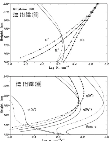
Fig. 8.Same as Fig. 3, but for a positive disturbance on 11 Jan/14 Jan 1990 with a height decreasing storm effect (top) and calculated ion production rates for this case (bottom).
6 Discussion
Incoherent scatter observations are known to provide the most complete and consistent information on ionospheric plasma in the F-region. ObservedN e(h)profiles were used in the paper for the analysis of the morphology of F1-layer storm effects. Our self-consistent method was successfully used for the physical interpretation of the storm effects. Nevertheless, some problems should be mentioned in rela-tion with the use of IS observarela-tions. Unlike ground-based ionosonde data the IS observations are irregular in time and it is not always possible to find a suitable combination of disturbed/quiet days for the analysis; therefore, the usable amount of data is limited. The quality of the experimental material is different at Millstone Hill and EISCAT. Due to rare (usually 3 per hour) observations at Millstone Hill, we had to use a 3–4 h period to calculate median profiles. It is not always possible (especially for disturbed days) to find a 3–4 h period around noon of relative stability inNmF2 and
observa-tions can be used for our model calculaobserva-tions.
Another well-known general problem with IS observations is related to the ion composition, and this is especially im-portant in case of the F1-layer data analysis. Experimen-tal T e(h), T i(h) andN e(h) profiles derived from the in-coherent scatter data analysis depend on the ion composi-tion used in the fit of the theoretical to the measured auto-correlation function (ACF). An uncertainty in ion compo-sition may lead to considerable uncertainties in the derived T e(h) andT i(h) profiles and to somewhat smaller uncer-tainties inN e(h)(e.g. Waldteufel, 1971; Lathuill`ere et al., 1983). The effect of varying ion composition is most no-ticeable during disturbed periods, but an appreciable effect may also take place for quiet periods as well (e.g. 6 July 2000). The largest uncertainties take place at the F1-region heights, where the ion composition changes from molecular to atomic one. Therefore, a correction of the experimental T e(h),T i(h)andN e(h)profiles is required. A simple cor-rection proposed by Waldteufel (1971) may be applied when the deviations in ion composition from the model (used in the IS data analysis) are not large, but in the case of strong pertur-bations, such as those present in the July 2000 event (Fig. 7), this simple correction results in unrealT e(h)andT i(h) pro-files. In such cases a more sophisticated iterative method considered by Mikhailov and Schlegel (1997) should be ap-plied, which provides the proper fit to the measured ACF. This iterative method requires considerable calculations and cannot be applied routinely.
EISCAT observations (each particular experiment) are not normalized by foF2 values. Although the declared uncer-tainty in the measured electron concentration is not large −10÷12% (Farmer et al., 1984; Kirkwood et al., 1986), this may result in wrong relative deviationsδN e when dif-ferent (quiet/disturbed) days are compared. The absence of such normalization also results in a shift between long-pulse and multi-pulseN e(h)profiles, and this shift should be taken into account before the profiles are used for analysis. Un-fortunately, foF2 data (due to problems with ground-based ionosonde observations in the auroral zone) are not available in some interesting cases, and one has to use IS observations, as they are without normalization. Despite the problems en-countered, the IS observations provide necessary information to specify physical mechanisms of the F1-layer storm effects, and this was implemented using our self-consistent method.
Among the observed storm features at mid-latitudes, the most interesting is a seasonal difference with a less pro-nounced summer storm effect compared to other seasons. This implies a seasonal difference in the thermosphere re-action to geomagnetic disturbances with the summer [O2] and[N2] increase, larger than the winter one (see Table 6 for 1log[O2] and 1log[N2] and Fig. 5 for 1q(N+2) and 1q(O+2)). The MSIS-86 model (Hedin, 1987) gives very small seasonal differences in1[O2]and1[N2], even at the F2-region heights (280 km) and practically negligible1[O2] and1[N2]variations in the F1-region (180 km). On the other hand, the ESRO-4 observations (Pr¨olss and von Zahn, 1977)
show a seasonal difference in1(N2/O)at 280 km for middle latitudes and daytime hours (their Fig. 4). According to the model of thermospheric composition by Zuzic et al. (1997) based on the ESRO-4 observations, larger N2/O disturbance intensity corresponds to larger1[N2]and smaller1[O], al-though the latter demonstrates large scatter (their Fig. 6). This seasonal difference in the thermospheric reaction may be attributed to the enhanced Joule heating in summer and to the storm-induced/background thermospheric winds interac-tion (e.g. Fuller-Rowell and Codrescu, 1996).
Unlike the F2-layer, where the role of dynamical processes (thermospheric winds, in particular) is essential, the elec-tron concentration in the F1-region (heights below 200 km) is controlled by photochemical processes. Therefore, the ob-servedN eF1 variations just reflect the variations of neutral composition and temperature. By analogy with the F2-layer (Pr¨olss, 1993), a decrease in the O/(N2+O2)ratio results in the negative storm effect, while F1-layer positive storm effect may be due to some other mechanisms. In particular, the positive storm effect at F1-layer heights on 15 July 2000 is mostly due to the atomic oxygen increase, as our analysis has shown. The height decreasing positive storm effect on 11 January 1990 (Fig. 8), on the other hand, was shown to be due to a thermosphere contraction below 220 km which resulted in a decrease of neutral concentrations at a given height (e.g. at 180 km in Table 6). This decrease in neutral atmosphere density has clearly appeared in the total ion production rate (Fig. 8, bottom). Theq(h)profile is shifted down as a whole without change in the maximum production rate. Such type of neutral atmosphere variation may be related to a passage of planetary or gravity waves during disturbed periods (e.g. Burns and Killeen, 1992).
7 Conclusions
Our morphological analysis of the storm effects at F1-layer heights (160–200 km) using EISCAT and Millstone Hill in-coherent scatter observations followed by physical interpre-tation has shown the following.
The morphological results:
1. The storm effects inN emay be positive and negative, but negative deviations prevail for all seasons. The mag-nitude of the positive effect is smaller compared to the negative one.
2. Usually, the amplitude of deviation increases with height, but the inverse type of dependence may also take place.
3. There is a direct and significant correlation between δN eat the F1-layer heights andδN mF2, the correlation coefficients increasing with height.
4. At middle latitudes the summer storm effect is less com-pared to other seasons, but it is well detectable. In the auroral zone this summer effect takes place only with respect to the autumnal period, while a spring/autumn asymmetry in the storm effect is well pronounced. 5. The F1-region exhibits a relatively small reaction to
geomagnetic disturbances despite large storm perturba-tions in the thermospheric parameters at the heights in question.
As the F1-region is formed, where both atomic O+ and molecular M+=O+
2 +NO+ ions strongly contribute to electron concentrationN e, the competition between1[O+] and1[M+] contributions explains the main morphological features, in particular:
6. Normally[O+]decreases while[M+]always increases in disturbed conditions. The[O+]decrease usually pre-vails (especially during equinoxes and in winter) and this determines the negative sign of the storm effect ob-served in the majority of cases. The summer[M+] in-crease is larger compared to the winter one, and the re-sultant negative storm effect is smaller in summer due to this compensation. The latter is related to seasonal dif-ferences in the thermosphere reaction to geomagnetic disturbances, with the summer[O2]and[N2]increase larger than the winter one. This revealed seasonal effect is confirmed by ESRO-4 neutral composition observa-tions for disturbed condiobserva-tions.
7. The small sensitivity of the F1-region to geomagnetic disturbances compared to the F2-layer one is also ex-plained in the framework of this mechanism. There is partial compensation (in winter and equinoxes) or prac-tically complete (in summer) compensation of negative 1[O+] by positive 1[M+] at F1-layer heights, while the pure1[O+]effect takes place in the F2-region.
8. The concentration of O+ ions increases with height, while[M+]demonstrates small height variations in the F1-region. Therefore, [O+] begins to dominate over [M+]in the upper part of the F1-region and above in the F2-region. Usually,1[O+]controls the sign of the F1-layer storm effect, and this explains both the increase of the storm effect with height and the direct (significant) correlation betweenδN eandδN mF2.
9. Small, positive storm effects also observed in the F1-region may result from different reasons. The increase of atomic oxygen abundance results in a positive ef-fect with a height increasing magnitude. A contraction of the lower thermosphere (presumably due to gravity waves) results in a height decreasing positive storm ef-fect.
10. In summary one may conclude that all the observed F1-layer storm effects may be related to seasonal and storm-time variations of neutral composition (O, O2, N2). The present day understanding of the F1-region formation mechanisms is sufficient to explain the ob-served storm effects.
Acknowledgements. The authors thank the Millstone Hill Group of the Massachusetts Institute of Technology, Westford; also the Di-rector and the staff of EISCAT for running the radar and providing the data. The EISCAT Scientific Association is funded by scien-tific agencies of Finland (SA), France (CNRC), Germany (MPG), Japan (NIPR), Norway (NF), Sweden (NFR), and the United King-dom (PPARC). A. V. Mikhailov is grateful to the Max-Planck-Gesellschaft for a research stipend at the MPAE.
Topical Editor M. Lester thanks C. Huang and another referee for their help in evaluating this paper.
References
Antonova, L. A. and Ivanov-Kholodny, G. S.: The F1-layer. Condi-tions for appearance and height, Geomagn. Aeronom., 28, 813– 816, 1988a.
Antonova, L. A. and Ivanov-Kholodny, G. S.: The F1-layer. De-pendence of electron concentration at the layer maximum on he-liogeophysical conditions, Geomagn. Aeronom., 28, 817–819, 1988b.
Banks, P. M. and Kockarts, G.: Aeronomy, Academic Press, New York, London, 1973.
Basu, S., Basu, Su., Groves, K. M., Yeh, H.-C., et al.: Response of the equatorial ionosphere in the South Atlantic region to the great magnetic storm of 15 July 2000, Geophys. Res. Lett., 18, 3577–3580, 2001.
Bilitza, D. (Ed): International Reference Ionosphere IRI-90, URSI-COSPAR, Rep. NSSDC/WDC-A Rocket and Satellites, Green-belt, USA, 1990.
Buonsanto, M. J.: Ionospheric storms – A review, Space Sci. Rev. 88, 563–601, 1999.
Buresova, D. and Lastovicka, J.: Changes in the F1-region elec-tron density during geomagnetic storms at low solar activity, J. Atmos. Solar-Terr. Phys., 63, 537–544, 2001.
Burns, A. G. and Killeen, T. L.: The equatorial neutral thermo-spheric response to geomagnetic forcing, Geophys. Res. Lett., 19, 977–980, 1992.
Danilov, A. D. and Lastovicka, J.: Effects of geomagnetic storms on the ionosphere and atmosphere, Int. J. Geomagn. Aeronom., 2, 209–224, 2001.
Farmer, A. D., Lockwood, M., Horne, R. B., Bromage, B. J. I., and Freeman, K. S. C.: Field-perpendicular and field-aligned plasma flows observed by EISCAT during a prolonged period of north-ward IMF, J. Atmos. Terr. Phys., 46, 473–488, 1984.
Fuller-Rowell, T. J. and Codrescu, M. V.: On the seasonal response of the thermosphere and ionosphere to geomagnetic storms, J. Geophys. Res., 101, 2343–2353, 1996.
Goldberg, R. A. and Blumle, L. J.: Positive composition from a rocket-borne mass-spectrometre, J. Geophys. Res., 75, 133–142, 1970.
Hedin, A. E.: MSIS-86 thermospheric model, J. Geophys. Res., 92, 4649–4662, 1987.
Hierl, P. M., Dotan, I., Seeley, J. V., Van Doran, J. M., Morris, R. and Viggiano, A. A.: Rate coefficients for the reactions ofO+
withN2andO2as a function of temperature (300–1800 K), J. Chem. Phys., 106, 9, 3540–3544, 1997.
Hubert, D. and Kinzelin, E.: Atomic and molecular ion tempera-tures and ion anisotropy in the auroral F-region in the presence of large electric fields, J. Geophys. Res., 97, 1053–1059, 1992. Ivanov-Kholodny, G. S. and Nikoljsky G. M.: The Sun and the
Ionosphere, Nauka, M., 335, in Russian, 1969.
Ivanov-Kholodny, G. S., Mikhailov, A. V., and Ostrovsky, G. I.: Day-to-day change in the summer values ofhmF2 andNmF2 as a reflection of variations in the neutral composition of the upper atmosphere, Geomagn. Aeronom., 21, 615–617, 1981.
Kirkwood, S., Collis, P. N., and Schmidt, W.: Calibration of elec-tron densities for EISCAT UHF radar, J. Atmos. Terr. Phys., 48, 773–775, 1986.
Lathuill`ere, C., Lejeune, G., and Kofman, W.: Direct measurements of ion composition with EISCAT in the high-latitude F1-region, Radio Sci., 18, 887–893, 1983.
Lathuill`ere, C. and Brekke, A.: Ion composition in the auroral iono-sphere as observed by EISCAT, Ann. Geophysicae, 3, 557–568, 1985.
Mikhailov, A. V.: Ionospheric F2-layer storms, Fisica de la Tierra, 12, 223–262, 2000.
Mikhailov, A. V. and Foster, J. C.: Daytime thermosphere above Millstone Hill during severe geomagnetic storm, J. Geophys. Res., 102, 17,275–17,282, 1997.
Mikhailov, A. V. and F¨orster, M.: Day-to-day thermosphere param-eter variation as deduced from Millstone Hill incoherent scatter radar observations during 16–22 March 1990 magnetic storm pe-riod, Ann. Geophysicae, 15, 1429–1438, 1997.
Mikhailov, A. V. and F¨orster, M.: Some F2-layer effects during the 6–11 January 1997 CEDAR storm period as observed with the Millstone Hill incoherent scatter facility, J. Atmos. Solar-Terr. Phys, 61, 249–261, 1999.
Mikhailov, A. V. and Kofman, W.: An interpretation of ion com-position diurnal variation deduced from EISCAT observations, Ann. Geophysicae, 19, 351–358, 2001.
Mikhailov, A. V. and Schlegel, K.: Self-consistent modeling of the daytime electron density profile in the ionospheric F-region, Ann. Geophysicae, 15, 314–326, 1997.
Mikhailov, A. V. and Schlegel, K.: Physical mechanism of strong negative storm effects in the daytime ionospheric F2-region ob-served with EISCAT, Ann. Geophysicae, 16, 602–608, 1998.
Mikhailov, A. V. and Schlegel, K.: A self-consistent estimate of
O++N2rate coefficient and total EUV solar flux withλ1050 ˚A using EISCAT observations. Ann. Geophysicae, 18, 1164–1171, 2000.
Mikhailov, A. V. and Schlegel, K.: Equinoctial transitions in the ionosphere and thermosphere, Ann. Geophysicae, 19, 783–796, 2001.
Nusinov, A. A.: Models for prediction of EUV and X-ray solar ra-diation based on 10.7 cm radio emission., Proc. Workshop on So-lar Electromagnetic Radiation for SoSo-lar Cycle 22, Boulder, Co., July 1992, (Ed) Donnely, R. F., NOAA ERL. Boulder, Co., USA, 354–359, 1992.
Oliver, W. L.: Models of the F1-region ion composition variations, J. Atmos. Terr. Phys., 37, 1065–1076, 1975.
Pavlov, A. V. and Foster, J. C.: Model/data comparison of F-region ionospheric perturbation over Millstone Hill during the severe geomagnetic storm of 15–16 July 2000, J. Geophys. Res., 106, 29 051–29 069, 2001.
Pollard, J. H.: A handbook of numerical and statistical techniques, Camb. Univ. Press, 1977.
Pr¨olss, G. W.: On explaining the local time variation of ionospheric storm effects, Ann. Geophysicae, 11, 1–9, 1993.
Pr¨olss, G. W.: Ionospheric F-region storms, in Handbook of Atmo-spheric Electrodynamics, Vol. 2 (Ed) Volland, CRC Press/Boca Raton, 195–248, 1995.
Pr¨olss, G. W. and von Zahn, U.: Seasonal variations in the latitudi-nal structure of atmospheric disturbances, J. Geophys. Res., 82, 5629–5632, 1977.
Richards, P. G. and Torr, D. G.: Ratios of photoelectron to EUV ion-ization rates for aeronomic studies, J. Geophys. Res., 93, 4060– 4066, 1988.
Richmond, A. D.: Upper-atmospheric effects of magnetic storms: a brief tutorial, J. Atmos. Solar-Terr. Phys., 62, 1115–1127, 2000. Shchepkin, L. A.: Some patterns in the vertical distribution of elec-tron and ion concentrations at heights between 130–200 km, Ge-omagn. Aeronom., 9, 380–384, 1969.
Shchepkin, L. A., Shuyskaya, Z. I., and Koshelev, V. V.: Estimation of the seasonal variation of the gas concentration at the height of the F1-layer from data on the conditions of its development, Geomagn. Aeronom., 12, 870–872, 1972.
Shchepkin, L. A. and Vinitzky, A. V.: Derivation of thefoF1 char-acteristic from ionograms, Geomagn. Aeronom., 21, 257–258, 1981.
St.-Maurice, J.-P. and Schunk, R. W.: Ion velocity distributions in the high-latitude ionosphere, Rev. Geophys. Space Phys., 17, 99– 134, 1979.
Torr, M. R., Torr, D. G., Ong, R. A., and Hinteregger, H. E.: Ionoza-tion frequencies for major thermospheric constituents as a func-tion of solar cycle 21, Geophys. Res. Lett., 6, 771–774, 1979. Vinitzky, A. V., Sukhomazova, G. I., and Shchepkin, L. A.:
Rela-tionship between the properties of the ionospheric F2- and F1-layers in the day-to-day variations, Geomagn. Aeronom., 22, 707–709, 1982.
Waldteufel, P.: Combined incoherent scatter F1-region observa-tions, J. Geophys. Res., 76, 6995–6999, 1971.
Zevakina, R. A., Goncharova, E. E., Pushkova, G. N., and Yo-dovich, L. A.: Effect of the ring current on on ionospheric F-region disturbance, Geomagn. Aeronom., 11, 825–829, 1971. Zuzic, M., Scherliess, L., and Pr¨olss, G. W.: Latitudinal structure of