Dynamic evolution of vortex dipoles
(Evoluci´on din´amica de dipolos vorticosos)E. Salinas-Rodr´ıguez
1, M.G. Hern´
andez
2, A. Torres
1, F. Valderrama
3and F.J. Vald´
es-Parada
11
Departamento de Ingenier´ıa de Procesos e Hidr´aulica, Universidad Aut´onoma Metropolitana, Iztapalapa, M´exico, D.F., M´exico.
2
Divisi´on de Ciencias B´asicas e Ingenier´ıa, Universidad Aut´onoma Metropolitana, Azcapotzalco, M´exico, D.F., M´exico 3
Departamento de Ingenier´ıa El´ectrica Universidad Aut´onoma Metropolitana, Iztapalapa, M´exico, D.F., M´exico
Recebido em 8/11/2010; Aceito em 16/6/2011; Publicado em 7/10/2011
Vortex dipoles are fundamental in fluid mechanics. They are found in geophysics, engineering and industry. The two necessary conditions to generate them are a plane flow and a generating force. In this work, an ex-perimental design to generate vortex dipoles in stratified beds is presented. Vortex rings were generated under different volumetric flow conditions. Through visualization techniques, three stages were observed during the evolution of the rings: an exponential stage associated with the injection of the tracer, a parabolic stage and finally a dissipative stage. From the experimental results, the Reynolds and P´eclet numbers were computed indicating laminar flows and diffusive flows, respectively.
Keywords: vortex dipoles, visualization techniques, Reynolds number, P´eclet number, stratified bed.
Los dipolos vorticosos son fundamentales en mec´anica de fluidos. Se encuentran en geof´ısica, ingenier´ıa y la industria. Las dos condiciones necesarias para generarlos son un flujo plano y una fuerza generadora. En este trabajo se presenta un dise˜no experimental para generar dipolos vorticosos en lechos estratificados. Se gene-raron anillos vorticosos bajo diferentes condiciones de flujo volum´etrico. Durante la evoluci´on de los anillos se observaron tres etapas, mediante t´ecnicas de visualizaci´on: una etapa exponencial asociada con la inyecci´on del trazador, una etapa parab´olica y finalmente una etapa disipativa. A partir de los resultados experimentales se calcularon los n´umeros de Reynolds y P´eclet e indicaron flujos laminares y difusivos, respectivamente.
Palabras-clave: dipolos vorticosos, t´ecnicas de visualizaci´on, n´umero de Reynolds, n´umero de P´eclet, lecho estratificado.
1. Introduction
A vortex dipole is an axial flow with two vortices of equal strength but opposite sign travelling through a fluid. Due to the fluid’s viscosity, the vorticity spreads over a larger area and therefore, the dipole decreases in strength, it slows down and spirals towards the cen-tre of the domain. Inside the dipole, the fluid flows along the streamlines, around the extreme of vorticity; the maximum velocity, in the positive xdirection, oc-curs at the dipole axis [1]. One half of the dipole has positive vorticity, whereas the other half has negative vorticity, therefore its total circulation is zero. Outside this circle there is no vorticity and the flow is poten-tial. Vortex dipoles are very stable structures and decay only when their kinetic energy is almost completely dis-sipated by friction. Analytically, the dipole dynamics had been studied through the Navier-Stokes equation,
considering different initial conditions, since its solution depends strongly on them.
The vortex dipoles are fundamental elements in the dynamics of complex fluids and take place in natural systems. They have been observed in the oceans and in the atmosphere [2], in airfoils [3-5], in animals as jellyfish and squid for propulsion [6], in plants growth and in spore spread [7]. Therefore, their application in-cludes diverse areas of physics and engineering as: me-teorology, aerodynamics, biology, super-fluids and in-dustrial turbulent flows [8-9]. Their motions are prac-tically bidimensional due to the presence of stratified fluids, the rotation of the system, or by the combina-tion of both factors. In order to generate them, two conditions are necessary: a plane flow and a generat-ing force [10-12]. Therefore, understandgenerat-ing the vortex dipole generation and dynamics is of great interest in physics and engineering.
1
E-mail: [email protected].
In this work a vortex dipole is generated by a hor-izontal impulse into a stratified fluid. The vorticity is advected (transport due to the motion of the fluid the particle is suspended in) by the induced flow and dif-fuses (movement of particles along concentration gra-dients). The basic purpose of this work is to present a simple and economical experimental design to gener-ate dipole rings. To this end the article is organized as follows. Section 2 is devoted to the experimental equipment design. In Section 3 we present the results of our experiments and in Section 4 we summarize our conclusions and discuss the scope and limitations of our work.
2.
Experimental set-up and procedures
2.1. Experimental set-up and procedure
The experimental set-up consists of a container with its corresponding nozzle, and a measuring technique. Each component is explained in detail below.
2.2. Experimental container
The experiments were performed in a rectangular acrylic container 0.3 x 0.15 x 0.06 m and 0.012 m in wall thickness. A container with marble grain and a base of compacted rubber foam was used to avoid ex-ternal disturbances during the experiments. Besides, the lamps container had an aired system to maintain constant the temperature of the fluids. The container was linearly stratified with common salt by diluting 80 g of salt per water liter. Distilled water was used as displacing fluid and food colorant (17 McCORMICK) was used as the displaced fluid. The fluids properties were measured at T= 24 ± 0.5 ◦C, the temperature,
T, of the fluids and the interface were controlled by thermocouples type “J” of Constantan Iron (Kew In-dustries), through a digital analogical card of data ac-quisition (National Instruments) and Virtual software Bench- Logger. The shear viscosities of water and col-orant wereµw= 0.0010019 Pa.s andµt= 0.01632 Pa.s (Ostwald viscometer), respectively. Interfacial tension between water and colorant was σ = 58 x 10−3 N/m (Fisher tensiometer). The densities were ρw = 997 kg/m3 for water and ρ
t = 1105.48 kg/m3 for the col-orant (analytical balance, Ohaus). The container di-ameter was large enough so that wall effects can be as-sumed negligible. In Fig. 1 the schematic experimental apparatus is shown. The stratified bed was done with 850 x 10−6 m3 of saline water and it was added in the container. The tracer liquid was injected to generate a horizontal jet flow from the nozzle. Later on, a vege-tal sheet of paper was placed on it and 275 x 10−6 m3 of distilled water was carefully poured the sheet until
slightly cover the nozzle; finally, the sheet was carefully removed [10].
Figure 1 - Experimental set-up.
The tracer liquid was previously stored in a con-tainer and it was supplied with a regulated water pump (Jideco, model MC2-12) that generates a volumetric flow of (65.5 ± 0.001) x 10−6 m3/s, impelled with a motor of 12 V (CD) and a power of 29 x 10−3 Hp [13]. With a voltage source (Tektronix), the power necessary for the impelling motor of the pump was characterized resulting in the ability to control the volumetric flow with the opening of a control valve (Guss & Roch), ob-taining volumetric flows from (3±0.001) x 10−9 m3/s to (25 ±0.001) x 10−9 m3/s through the nozzle. This automatized injection system controls the volumetric flow very precisely. It must be stressed that in Ref. [3] the tracer liquid was supplied by a burette manipula-tion. In Fig. 2, the hydraulic circuit is schematically shown.
Figure 2 - Components of the hydraulic circuit.
fluid on it, these adhesions could change the initial con-ditions of the system.
Figure 3 - Bronze nozzle (a) Squematic figure, (b) Photograph.
2.3. Technique of visualization and images
treatment
The formation and evolution of the vortex ring was recorded with a video camera (Sony, CCDF50) at 30 frames per second. In order to avoid undesired reflec-tions and shadows, as much as possible, a specific light-ning array with four white light tubes was placed on a wood container; some orifices were made on it to avoid overheating. Also, a container with marble grain and a base of compacted rubber foam were placed bellow this array, to avoid external disturbances. The experiment took place in an entirely controlled environment. Ten experiments for three different volumetric flows: Q0 = 10.4 x 10⁻⁹ m3/s, Q
1 = 11.0 x 10⁻⁹ m3/s and Q2 = 14.5 x 10⁻⁹m3/s were done. The images were digitized directly from the camera and later on, they were pro-cessed with AVI and DUB software. Finally individual frames were processed with the picture software Corel Draw 14, to obtain the data of each experiment.
3.
Results and discussion
From the complete set of images, there were only con-sidered those corresponding to each second. The first step in the analysis was to establish the beginning and end of the phenomena. The beginning of an experiment
was selected as the frame before the first displacement of the colorant. In addition, the end of an experiment was set up to correspond to the instant when the trans-verse displacement of the vortex ring reached a steady state. As a frame of reference, this instant was fixed to correspond to a distance of 4.5 cm from the noz-zle in all cases. The second step was to calibrate the measurement of the longitudes. To this end the cor-responding relation between the length measured from each image frame and the physical length were derived, by using the millimetric paper placed below the exper-imental container (Fig. 4).
Figure 4 - Dipole ring.
Afterwards, the length and width of a vortex ring can be directly measured; as the rings were formed, the front of the transversal diameter of the ring was selected as the point for the measurements of transversal length. It is important to mention that the data treatment was made considering the trajectory along the center line, therefore if the dipole rings deviated from it, the uncer-tainty of the data increased.
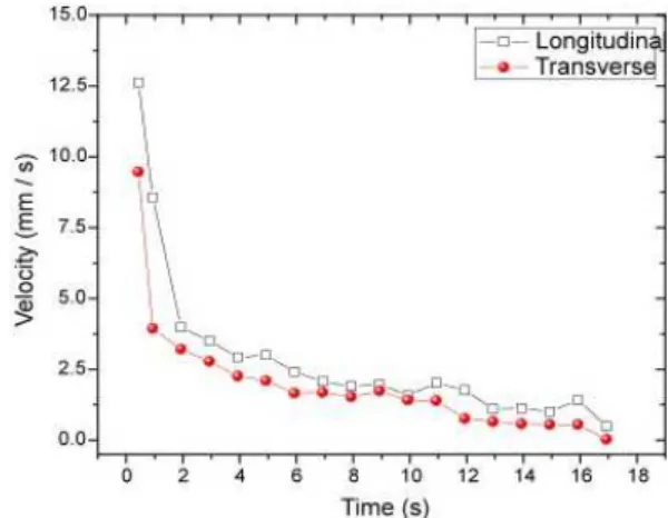
An example of the measurements for Q2 is shown in Fig. 5. It must be stressed that the transverse dis-placement reaches the steady state before its longitu-dinal counterpart. Similar results were observed in the other experiments.
With these results the velocity can be computed
vi,j=
Li,j−Li−1,j ti−ti−1
, j =L, T, (1)
as well as the average velocity
⟨v⟩j = 1
N i∑=N
i=1
Li,j−Li−1,j ti−ti−1
, j=L, T, (2)
whereN is the number of data.
An example of the evolution of the longitudinal⟨v⟩L and transverse⟨v⟩T components of the velocity is shown in Fig. 6. As expected, both velocities decrease with time, indicating a deceleration of the colorant spread-ing. The average velocities, computed using Eq. (2), were algebraically averaged to obtain the results shown
in Table 1. The uncertainty is one order of magnitude smaller than the computed velocity.
Figure 6 - Longitudinal and transverse velocityvs. tforQ1.
⌋
Table 1 - Average longitudinal and transverse velocity for each flow rate.
Volumetric flow (m3
/s) ⟨v⟩L(m/s) ⟨v⟩T(m/s) ⟨v⟩T/⟨v⟩L
Q0 0.00177±0.0006 0.00113±0.0003 0.638±0.05
Q1 0.00295±0.0000 0.00209±0.0001 0.708±0.03
Q2 0.00304±0.0002 0.00215±0.0002 0.707±0.07
⌈
From these results it can be appreciated that ⟨v⟩T
is always smaller than ⟨v⟩L, it is consistent with the fact that viscosity spreads the vorticity over the area and thus slows down each monopole. Also, the rate
⟨v⟩T/⟨v⟩LforQ2is lower thanQ1, in contrast than we expect, nevertheless it is important to remember that the uncertainties for the velocities in the experiment 2 are bigger than in the experiment 1.
Since there is a concentration gradient, there is a diffusion process that obeys Ficks’s law, and the diffu-sion coefficient D of the water-colorant system can be obtained in a crude estimation as
D= 1
N i∑=N
i=1
LiLi−1
ti−ti−1
. (3)
It is important to stress thatD is an average quan-tity, in the sense that strictly, it should be is defined as a statistical average over an ensemble with a number of molecules around the Avogadro number. In this work, we only considered two thousand frames to compute the axial diffusion and the results are given in Table 2. It can be observed that the uncertainty is one order of magnitude smaller than the computed diffusion coef-ficient. Nevertheless, the uncertainty for Q0 is greater than forQ1andQ2, the reason of it could be the devia-tion of the path from its center line. It must be stressed that this deviation could be produced by the external noise that are of the same order than the dynamic force
induced by Q0.
Table 2 - Diffusion coefficient.
Q(m3
/s) Q0 Q1 Q2
Dx 105
(m2
/s) 1.27±1.3 1.70±0.316 1.96±0.5
From Tables 1 and 2 it is evident that the best data belongs to theQ1, and the uncertainty was lower than the other volumetric flows, for this stratified bed. More-over, the best dipoles rings were developed for this flow; for the lowest, Q0, the dipole rings deviated from the center line.
The Reynolds number Re = ρw⟨v⟩dn/µw that establishes the relation between inertial and viscous forces, the P´eclet number P e ≡ ⟨v⟩dn/D that gives the ratio between inertial and diffusive effects, and the Schmidt number that gives the ratio between viscous and diffusive effects, Sc ≡µw/(ρwD) = P e/Re, were computed for the three volumetric flows. These num-bers indicate the relative importance of two dynamical processes. The results are reported in Table 3.
Table 3 - Reynolds, P´eclet and Schmidt numbers for different volumetric flows.
Re Re Pe Sc
Q0 1.09 0.62 0.08 0.07
Q1 1.33 0.92 0.07 0.05
Q2 1.12 0.92 0.05 0.05
dipoles vortex it is usually considered that the flow is laminar when the Reynolds number is lower than 100 [15]. As can be seen in Table 3, Reynolds number is between 0.693 and 1.497, therefore the flow regime is laminar. On the other hand, the P´eclet number is be-tween 0.079 and 0.115, so the inertial forces are 0.79% to 11.5% greater than diffusive forces. It can be seen that Pe1 < Pe2, but it is in the range of the exper-imental uncertainties values. The Schmidt number is between 0.053 and 0.166, indicating that the viscous effects are 5.3% to 16.6% greater than the diffusive ef-fects. These values suggest that there is a diffusive flow, which might be due to the fact the tracer fluid’s viscos-ity is sixteen times larger than that of water.
4.
Conclusions
In this work, a simple and economical experimental de-sign to generate vortex rings in a stratified bed was presented, following the Afasanayev design [10], but introducing an automatized injection system and an antivibrational aired container. The former allows an accurate experiment’s repeatability. The latter avoid the interaction between the external vibrations and the dipole dynamics.
The longitudinal and transversal longitudes were obtained with different visualization techniques and they were digitally analyzed. The software used is ac-cessible at undergraduate and graduate courses. This experiment allows the students: to generate the vor-tex dipoles; to identify the parameters involved such as temperature, saline concentration, volumetric flow and the nozzle’s internal diameter. The student also learns to analyze results with statistical methods.
The best vortex dipole corresponds to the largest volumetric flow. Nevertheless, the volumetric flow is of marginal importance in the dipoles average velocity for the saline concentration considered. Therefore, it is of importance to consider different saline concentra-tions in further work, as well as temperature gradients. Reynolds numbers showed laminar flows and the P´eclet and Schmidt numbers showed diffusive flows.
The essential point to stress, though, is that this type of experiments allow the students to identify dif-ferent flow regimes through the computed the obtained values of non-dimensional numbers as Reynolds, P´eclet and Schmidt. Also, it is possible to observe how the qualitative behavior in this experiment is the analog to processes in nature and industries.
References
[1] H.G.M. van Geffen, V.V. Meleshko and G.J.F. van Hei-jst, J Physics of Fluids8, 2393 (1996).
[2] D.G. Dritschel and B. Legras, Physics Today 46, 44 (1993).
[3] M.D. Blokhina and Y.D. Afanasyev, J Geophys Res Oceans108, 3322 (2003).
[4] http://alexl.wordpress.com/fascinating-flows/, acessed in July 1st
, 2010.
[5] J.H.B. Smith, Ann Rev Fluid Mech18, 221 (1986).
[6] J.O. Dabiri, Annu Rev Fluid Mech41, 17 (2009).
[7] D.L. Whitaker and J. Edwards, Science 329, 406 (2010).
[8] G.J.F. van Heijst, Nederlands voor Tijdschrift Natu-urkunde59, 321 (1993).
[9] R. Rajes and K. Mahesh, J Flow Mechanics 604, 389 (2008).
[10] Y. Afanasyev, Am J Phys70, 86 (2002).
[11] D.J. Acheson, Eur J Phys21, 269 (2000).
[12] O. Praud and A. Fincham, J Flow Mech544, 1 (2005).
[13] C.L. Philips and D. Harbor,Feedback Control of Sys-tems, Design and Analysis of Electrical Processes and Controller (Prentice Hall, Englewood Cliffs, 1996).
[14] F. Valderrama, E. Salinas-Rodr´ıguez, A. Torres and M.G. Hern´andez, Prototype: Design, Automatization and Construction of a Container for Vortex Rings Generation (Universidad Aut´onoma Metropolitana-Iztapalapa, Mexico City, 2009).
[15] F. Rooij, P.F. Linden and S.B. Dalziel, J Fluid Mech