❆♠❛✉r✐ ❍♦❧❛♥❞❛ ❞❡ ❙♦✉③❛ ❏ú♥✐♦r
❘❡❣✐♦♥❛❧ ▼♦❞❡❧s ❛♥❞ ▼✐♥✐♠❛❧ ▲❡❛r♥✐♥❣
▼❛❝❤✐♥❡s ❢♦r ◆♦♥❧✐♥❡❛r ❉②♥❛♠✐❝ ❙②st❡♠
■❞❡♥t✐✜❝❛t✐♦♥
❘❡❣✐♦♥❛❧ ▼♦❞❡❧s ❛♥❞ ▼✐♥✐♠❛❧ ▲❡❛r♥✐♥❣ ▼❛❝❤✐♥❡s ❢♦r
◆♦♥❧✐♥❡❛r ❉②♥❛♠✐❝ ❙②st❡♠ ■❞❡♥t✐✜❝❛t✐♦♥
A thesis presented to the Graduate Program of Teleinformatics Engineering at Federal Uni-versity of Cear´a in fulfillment of the thesis requirement for the degree of Doctor of Phi-losophy in Teleinformatics Engineering.
Federal University of Cear´a
Center of Technology
Graduate Program of Teleinformatics Engineering
Supervisor: Guilherme de Alencar Barreto
Dados Internacionais de Catalogação na Publicação Universidade Federal do Ceará
Biblioteca de Pós-Graduação em Engenharia - BPGE
S715r Souza Júnior, Amauri Holanda de.
Regional models and minimal learning machines for nonlinear dynamic system identification / Amauri Holanda de Souza Júnior. – 2014.
128 f. : il. color. , enc. ; 30 cm.
Tese (doutorado) – Universidade Federal do Ceará, Centro de Tecnologia, Departamento de Engenharia de Teleinformática, Programa de Pós-Graduação em Engenharia de Teleinformática, Fortaleza, 2014.
Área de concentração: Sinais e Sistemas.
Orientação: Prof. Dr. Guilherme de Alencar Barreto.
1. Teleinformática. 2. Aprendizagem supervisionada. 3. Modelagem não linear. I. Título.
Research and writing a Ph.D. thesis is not something one can do all by himself. Therefore, I would like to thank everyone who contributed to this thesis in one or many ways.
First of all, I am grateful to God for making this dream become true.
I had an excellent advisor, Dr. Guilherme A. Barreto, who gave me the opportunity to pursue my Ph.D. degree, accepting me as one of his students even though I came up to him without strong knowledge in the subject. Guilherme introduced me to a very interesting research topic, that I have followed during Master and Doctoral studies. Moreover, I would like to thank Guilherme for all the patient, advises and support over the last 5 years. Guilherme matched the thin line between give me freedom to have my ideas (mostly nonsense) and keep me focused in what is important to accomplish a Ph.D. degree.
I am indebted to my friend and co-advisor Dr. Francesco Corona for the inspiring discussions and for the proofreading of my thesis. Francesco had a fundamental importance regarding research decisions and directions.
I would also like to thank all my colleagues of GRAMA group (Ananda, Cesar, Daniel, Ajalmar, Gustavo, Z´e Maria, Everardo and David) for the stimulating work environment, the exchange of interesting ideas, and the relaxing talks.
Special thanks go to Dr. Amaury Lendasse, Dr. Yoan Mich´e and all members of the Environmental and Industrial Machine Learning (EIML) group for the hospitality during my internship at Aalto University in Finland.
I want to thank my colleagues at the Department of Computer Science at IFCE, for the daily talks, the respectable work environment, and the lunch times we had together.
CAPES for the financial support.
This thesis addresses the problem of identifying nonlinear dynamic systems from amachine learning perspective. In this context, very little is assumed to be known about the system under investigation, and the only source of information comes from input/output mea-surements on the system. It corresponds to the black-box modeling approach. Numerous strategies and models have been proposed over the last decades in the machine learning field and applied to modeling tasks in a straightforward way. Despite of this variety, the methods can be roughly categorized into global and local modeling approaches. Global modeling consists in fitting a single regression model to the available data, using the whole set of input and output observations. On the other side of the spectrum stands the local modeling approach, in which the input space is segmented into several small partitions and a specialized regression model is fit to each partition.
The first contribution of the thesis is a novel supervised global learning model, theMinimal Learning Machine(MLM). Learning in MLM consists in building a linear mapping between input and output distance matrices and then estimating the nonlinear response from the geometrical configuration of the output points. Given its general formulation, the Minimal Learning Machine is inherently capable of operating on nonlinear regression problems as well as on multidimensional response spaces. Naturally, its characteristics make the MLM able to tackle the system modeling problem.
The second significant contribution of the thesis represents a different modeling paradigm, calledRegional Modeling(RM), and it is motivated by theparsimonious principle. Regional models stand between the global and local modeling approaches. The proposal consists of a two-level clustering approach in which we first partition the input space using the Self-Organizing Map(SOM), and then perform clustering over the prototypes of the trained SOM. After that, regression models are built over the clusters of SOM prototypes, or regions in the input space.
Even though the proposals of the thesis can be thought as quite general regression or supervised learning models, the performance assessment is carried out in the context of system identification. Comprehensive performance evaluation of the proposed models on synthetic and real-world datasets is carried out and the results compared to those achieved by standard global and local models. The experiments illustrate that the proposed methods achieve accuracies that are comparable to, and even better than, more traditional machine learning methods thus offering a valid alternative to such approaches.
List of Figures
Figure 1 – The system identification pipeline. . . 21
Figure 2 – The two configurations for model’s operation. . . 25
Figure 3 – Artificial data created from Eq. (1.9). . . 27
Figure 4 – General structure of single-hidden layer feedforward networks. . . 35
Figure 5 – Illustration of a local modeling approach: modular architectures. . . 39
Figure 6 – Taxonomy of divide-and-conquer approaches. Blue circles denote lo-cal approximating methods whereas green circles represent modular architectures. . . 39
Figure 7 – Neighborhoods: a) JkN N x ={x1,x5,x6}, b) J ekN N x ={x1,x3,x5,x6,x8}, c) JxN N={x1,x2,x3,x5,x6}, and d) J N N i x ={x1,x2,x3,x5,x6,x7,x8,x9}. 45 Figure 8 – Illustration of the distance mapping in the MLM. . . 51
Figure 9 – Output estimation. . . 52
Figure 10 – Use of the MLM for nonlinear system identification: external dynamics approach. . . 56
Figure 11 – Selection of reference points through k-medoids. . . 57
Figure 12 – Selection of reference points through KS test for two different functions. 58 Figure 13 – The smoothed parity function: Data . . . 59
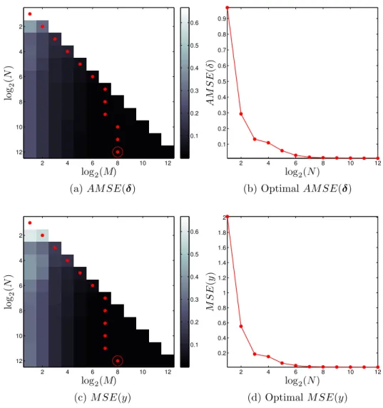
Figure 14 – The smoothed parity function: Figures of merit. . . 60
Figure 15 – The smoothed parity function: Output estimation with N = 212 and M = 28. . . . 61
Figure 16 – Synthetic example: MLM results. . . 62
Figure 17 – Synthetic example: MLM estimates. . . 62
Figure 18 – Synthetic example: MLM static behavior. . . 63
Figure 19 – Illustration of the regional modeling approach. . . 67
Figure 20 – Synthetic example: steps for the partitioning of the input space via regional modeling. . . 70
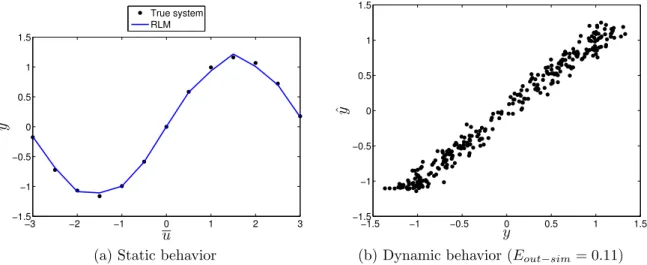
Figure 21 – Synthetic example: RLM results. . . 71
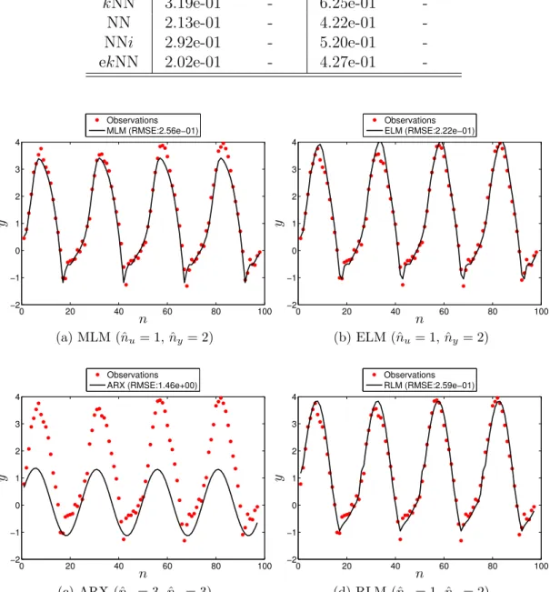
Figure 25 – Narendra’s plant: residual analysis for the MLM. . . 81
Figure 26 – Narendra’s plant: residual analysis for the ELM. . . 81
Figure 27 – Narendra’s plant: static behavior. . . 82
Figure 28 – pH dynamics: estimation/training data. . . 83
Figure 29 – pH dynamics: simulations on the validation set. . . 85
Figure 30 – pH dynamics: residual analysis for the MLM. . . 86
Figure 31 – pH dynamics: residual analysis for the RLM. . . 86
Figure 32 – Hydraulic actuator plant. . . 87
Figure 33 – Actuator plant: RMSE values on cross-validation per number of reference points. . . 88
Figure 34 – Actuator plant: simulations on the validation set. . . 89
Figure 35 – Hydraulic actuator: residual analysis for the MLM. . . 90
Figure 36 – Hydraulic actuator: residual analysis for the RLM. . . 90
Figure 37 – Heater system: input and output time-series. . . 91
Figure 38 – Heater: simulations on the validation set. . . 93
Figure 39 – Heater: residual analysis for the RBF. . . 94
Figure 40 – Heater: residual analysis for the RLM. . . 94
Figure 41 – The Tai Chi symbol: Data. . . 116
Figure 42 – The Tai Chi symbol: Figures of merit. . . 117
Figure 43 – The Tai Chi symbol: Output estimation, with N = 212 and M = 28. . . 118
Figure 44 – MLM cross-validation performance on classification. Legends also con-tain the total number of training samples. . . 120
List of Tables
Table 1 – Averages on validation performance (RMSE): Narendra’s plant. . . 80
Table 2 – Averages on validation performance (RMSE): pH dynamics. . . 84
Table 3 – Averages on validation performance (RMSE): Actuator. . . 88
Table 4 – Averages on validation performance (RMSE): Heater. . . 92
Table 5 – Description of the datasets: input/output dimensionality and number of training/test samples. . . 118
Table 6 – Test performance: accuracies (%), the corresponding standard deviations and Wilcoxon signed-ranks test results (X: fail to reject,×: reject). For each dataset, the best performing models are in boldface. . . 119
Table 7 – Description of the datasets: input/output dimensionality and number of training/test samples. . . 121
AMSE Averages on Mean Squared Error
ANFIS Artificial Neuro-Fuzzy Inference System
APRBS Amplitude Pseudo Random Binary Signal
ARX AutoRegressive with eXogenous input
DB Davies-Bouldin
ekNN Enclosing k Nearest Neighbors
ELM Extreme Learning Machine
GP Gaussian Processes
ITL Information Theoretic Learning
KDE Kernel Dependency Estimation
kNN k Nearest Neighbors
KS Kolmogorov-Smirnov test
LL Lazy Learning
LLM Local Linear Map
LLR Local Linear Regression
LMS Least Mean Squares
LOO Leave-One-Out
LS Ordinary Least Squares
MIMO Multiple-Input Multiple-Output
MLM Minimal Learning Machine
MLP Multi-layer Perceptrons
MSE Mean Squared Error
NARX Nonlinear AutoRegressive with eXogenous input
NN Natural Neighbors
NNi Natural Neighbors Inclusive
OPELM Optimally Pruned Extreme Learning Machine
RBF Radial Basis Functions
RLM Regional Linear Models
RLS Recursive Least Squares
RM Regional Modeling
RMSE Root Mean Squared Error
SLFN Single-hidden Layer Feedforward network
SVM Support Vector Machines
SVR Support Vector Regression
SISO Single-Input Single-Output
SOM Self-Organizing Map
TS Takagi-Sugeno
VQ Vector Quantization
X Set of input data points used for estimation.
Y Set of output data points used for estimation.
N Number of data points used for estimation.
x(n) Input vector at sampling time n.
y(n) Output observation at sampling time n.
X Input space.
Y Output space.
β Parameters of linear models.
wi i-th weight vector in Self-Organizing Maps.
rm m-th reference input point (MLM).
tm m-th reference output point (MLM).
ml l-th hidden unit (SLFN).
pi i-th k-means prototype
M Number of reference points (MLM).
L Number of hidden units (SLFN).
Q Number of SOM prototypes.
❈♦♥t❡♥ts
✶ ■♥tr♦❞✉❝t✐♦♥ ✳ ✳ ✳ ✳ ✳ ✳ ✳ ✳ ✳ ✳ ✳ ✳ ✳ ✳ ✳ ✳ ✳ ✳ ✳ ✳ ✳ ✳ ✳ ✳ ✳ ✳ ✳ ✳ ✳ ✳ ✳ ✳ ✳ ✳ ✶✾
1.1 The system identification problem . . . 19
1.1.1 Data acquisition . . . 21
1.1.2 Model structure selection . . . 22
1.1.3 Parameter estimation . . . 23
1.1.4 Model validation . . . 24
1.1.5 A synthetic example . . . 26
1.2 Objectives of the thesis . . . 27
1.3 Chapter organization and contributions . . . 28
1.4 Publications . . . 29
✷ ●❧♦❜❛❧ ❛♥❞ ▲♦❝❛❧ ▲❡❛r♥✐♥❣ ▼♦❞❡❧s ❢♦r ❙②st❡♠ ■❞❡♥t✐✜❝❛t✐♦♥ ✳ ✳ ✳ ✳ ✳ ✸✶ 2.1 Global modeling . . . 31
2.1.1 Least Squares and ARX models . . . 32
2.1.2 Single-hidden layer feedforward networks . . . 34
2.1.2.1 MultiLayer Perceptrons . . . 35
2.1.2.2 Extreme Learning Machines . . . 36
2.1.2.3 Radial Basis Function Networks . . . 37
2.2 Local modeling . . . 38
2.2.1 Modular architectures . . . 40
2.2.1.1 The Self-Organizing Map . . . 40
2.2.1.2 The Local Linear Map . . . 41
2.2.2 Local approximating models . . . 42
2.2.2.1 The VQTAM Approach . . . 42
2.2.2.2 The kSOM Model . . . 43
2.2.2.3 Local Linear Regression . . . 44
2.3 Conclusions . . . 46
✸ ❚❤❡ ▼✐♥✐♠❛❧ ▲❡❛r♥✐♥❣ ▼❛❝❤✐♥❡ ✳ ✳ ✳ ✳ ✳ ✳ ✳ ✳ ✳ ✳ ✳ ✳ ✳ ✳ ✳ ✳ ✳ ✳ ✳ ✳ ✳ ✳ ✹✼ 3.1 Basic formulation . . . 49
3.2 Parameters and computational complexity . . . 52
3.3 Links with Multiquadric Radial Basis Functions and Kernel Dependency Estimation . . . 55
3.6.1 The smoothed parity . . . 59
3.6.2 Synthetic example . . . 61
3.7 Concluding remarks . . . 62
✹ ❘❡❣✐♦♥❛❧ ▼♦❞❡❧✐♥❣ ✳ ✳ ✳ ✳ ✳ ✳ ✳ ✳ ✳ ✳ ✳ ✳ ✳ ✳ ✳ ✳ ✳ ✳ ✳ ✳ ✳ ✳ ✳ ✳ ✳ ✳ ✳ ✳ ✳ ✳ ✻✺ 4.1 Regional modeling by clustering of the SOM . . . 66
4.1.1 Illustrative example . . . 69
4.2 Outlier Robust Regional Models . . . 72
4.3 Related works . . . 73
4.4 Closing remarks . . . 74
✺ ❊①♣❡r✐♠❡♥ts ✳ ✳ ✳ ✳ ✳ ✳ ✳ ✳ ✳ ✳ ✳ ✳ ✳ ✳ ✳ ✳ ✳ ✳ ✳ ✳ ✳ ✳ ✳ ✳ ✳ ✳ ✳ ✳ ✳ ✳ ✳ ✳ ✳ ✳ ✼✼ 5.1 Methodology . . . 77
5.2 Example: Narendra’s plant . . . 78
5.3 Example: pH dynamics . . . 83
5.4 Identification of a hydraulic actuator . . . 87
5.5 Identification of a heater with variable dissipation . . . 91
5.6 Closing remarks . . . 92
✻ ❈♦♥❝❧✉s✐♦♥s ❛♥❞ ❋✉t✉r❡ ❉✐r❡❝t✐♦♥s ✳ ✳ ✳ ✳ ✳ ✳ ✳ ✳ ✳ ✳ ✳ ✳ ✳ ✳ ✳ ✳ ✳ ✳ ✳ ✳ ✳ ✾✺ 6.1 Future Directions on the Minimal Learning Machine . . . 97
6.2 Future Directions on Regional Modeling . . . 98
❇✐❜❧✐♦❣r❛♣❤② ✳ ✳ ✳ ✳ ✳ ✳ ✳ ✳ ✳ ✳ ✳ ✳ ✳ ✳ ✳ ✳ ✳ ✳ ✳ ✳ ✳ ✳ ✳ ✳ ✳ ✳ ✳ ✳ ✳ ✳ ✳ ✳ ✳ ✳ ✳ ✳ ✶✵✶ ❆PP❊◆❉■❳ ❆ ❈❧✉st❡r✐♥❣ ❛❧❣♦r✐t❤♠s ✳ ✳ ✳ ✳ ✳ ✳ ✳ ✳ ✳ ✳ ✳ ✳ ✳ ✳ ✳ ✳ ✳ ✳ ✳ ✳ ✶✶✶ A.1 k-means algorithm . . . 111
A.2 k-medoids algorithm . . . 112
A.3 Cluster validity indexes . . . 113
A.3.1 Davies-Bouldin index . . . 113
❆PP❊◆❉■❳ ❇ ▼✐♥✐♠❛❧ ▲❡❛r♥✐♥❣ ▼❛❝❤✐♥❡ ❢♦r ❈❧❛ss✐✜❝❛t✐♦♥ ✳ ✳ ✳ ✳ ✳ ✳ ✶✶✺ B.1 Formulation . . . 115
B.2 Illustrative example . . . 116
B.3 Experiments . . . 117
B.3.1 Results . . . 119
❆PP❊◆❉■❳ ❈ ▼✐♥✐♠❛❧ ▲❡❛r♥✐♥❣ ▼❛❝❤✐♥❡ ❢♦r ❘❡❣r❡ss✐♦♥ ✳ ✳ ✳ ✳ ✳ ✳ ✳ ✳ ✶✷✶ C.1 Experiments . . . 121
16
Chapter 1
Introduction
Modeling takes a central role in engineering and science in general. Almost all systems that someone can think of or imagine can be approximately described by a mathematical model (BILLINGS, 2013). Knowing a model that describes the diversity of behaviors that a dynamic system can reveal — particularly the nonlinear ones — is essential, not only for theoretic or applied research fields, but also for the process or control engineer who is interested in understanding better the dynamics of the system under investigation. The resulting model must approximate the actual system as faithfully as possible so that it can be used for several purposes, such as simulation, predictive control or fault detection.
This is an introductory chapter where we state the system identification problem to be addressed in this thesis in Section 1.1. In Section 1.2, we describe the objectives and motivations of the thesis. The structure of the thesis and contributions are reported in Section 1.3. Finally, in Section 1.4, the main scientific production during the Ph.D. course is presented.
✶✳✶ ❚❤❡ s②st❡♠ ✐❞❡♥t✐✜❝❛t✐♦♥ ♣r♦❜❧❡♠
An alternative way of describing dynamic systems is by finding a mathematical description of a dynamic system from empirical data or measurements in the system. This is usually referred to as the black-box modeling approach (SJ ¨OBERG et al., 1995), and it is the topic of this thesis. In cases where some partial a prior knowledge about the system is available while modeling it, such an approach stands between white-box and black-box modeling and it is said to be gray-box modeling (SOHLBERG, 2003).
A system is dynamic when its output at any time depends on its history, and not just on the current inputs. Thus, a dynamic system has memory and is usually described in terms of difference or differential equations. A single-input single-output dynamic system can be denoted by a set O= {u(n), y(n)}N
n=1 of inputs u(n) ∈R and outputs y(n)∈R
collected at sampling time n, and its input-output discrete time representation1 is given
by
y(n) = f(x(n)) +ǫ(n), (1.1) where x(n) represents the regression vector at sampling time n and its components are given as a function of the relevant variables of the system at previous time. Usually, x(n) encompasses past inputs and/or outputs and/or measurable disturbance observations. The additive term ǫ(n) accounts for the fact that the output observations y(n) may not be an exact function of past data.
The functionf :X→Yis the unknown, usually nonlinear, target function, whereX
denotes the input space, and Yis the output space. The ultimate goal in black-box system identification consists in finding a regression model h∈ H:X→Y that approximatesf in its entire domain, based on a finite set of measurements in the systemO. SetHdenotes the candidate models or hypotheses. Over the last decades, a number of learning models have been proposed to approximate or learn f, such as piecewise affine models (PAPADAKIS; KABURLASOS, 2010), neural networks (NARENDRA; PARTHASARATHY, 1990), fuzzy local models (TAKAGI; SUGENO, 1985; REZAEE; FAZEL ZARANDI, 2010), kernel-based methods (GREGORCIC; LIGHTBODY, 2008; ROJO-ALVAREZ et al., 2004), hybrid models (HABER; UNBEHAUEN, 1990; LIMA; COELHO; VON ZUBEN, 2007) and polynomial models (BILLINGS; CHEN; KORENBERG, 1989). Some of them will be discussed later in this thesis.
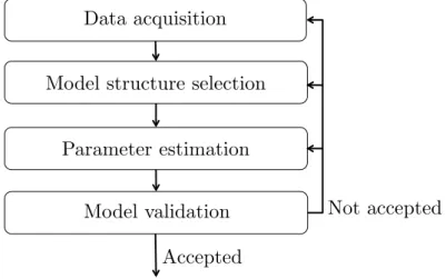
A common pipeline for identifying a dynamic system is illustrated in Figure 1. Basically, it includes: i) data acquisition; ii) model structure selection; iii) parameter estimation, and iv) model validation. The going backwards in Figure 1 occurs when the model is not appropriate, and then re-execution of previous stages is sometimes necessary to make a model adequate. In what follows, a brief description of each task within the system identification procedure is reported.
Chapter 1. Introduction 18
Model structure selection Data acquisition
Parameter estimation
Model validation
Accepted
Not accepted
Figure 1 – The system identification pipeline.
The algorithms used for black-box modeling of dynamic systems have mainly evolved in both automation/control and machine learning areas. Due to that, different nomenclatures are used as synonyms in many cases. Therefore, in order to avoid confusion with the nomenclature used in this thesis, we provide a glossary of equivalence between terms:
• estimate = train, learn;
• validate = test, generalize;
• estimation data = training data/set;
• validation data = generalization set, test set;
• in-sample error = training error;
• out-of-sample error = test error, generalization error.
✶✳✶✳✶ ❉❛t❛ ❛❝q✉✐s✐t✐♦♥
The first step consists of collecting data from the system with the objective of describing how the system behaves over its entire range of operation. It includes decisions on the sampling time and the input signal. The data acquisition procedure is usually done by applying an input control signal, u(n) ∈ R, to the system, and then observing the corresponding generated output, y(n)∈R. As a result of this process, we have a set of corresponding input and output observations O = {u(n), y(n)}N
n=1, where n denotes a
estimation step, since ill-conditioning regression matrices may be involved. Guidelines about the choice of the sampling rate of nonlinear systems are given by Aguirre (2007).
The quality of the model obtained is intimately related to the choice of the input signal used to excite the system. Ideally, the input-output time series should contain as much information as possible on the dynamics of the system. If nonlinearities are not present in the collected samples, it is impossible to learn the dynamics without any prior information about the system. The more complete and diverse the data is, the more feasible, from a learning point of view, the identification of the underlying system becomes. With respect to that, not only the frequency bands are important, but also amplitude information. The identification experiment which yields the data for the training set must be designed so that the input sequence excites the process dynamics as completely and uniformly as possible (BITTANTI; PIRODDI, 1996). To achieve this, white noise and amplitude pseudo random binary signal (APRBS) are commonly used.
There are many issues related to preliminary identification steps, such as pre-processing, normalization, nonlinearity detection, the choice of relevant variables in the system, etc. For a comprehensive discussion about such issues, we recommend the following texts: Nelles (2001) and Aguirre (2007).
✶✳✶✳✷ ▼♦❞❡❧ str✉❝t✉r❡ s❡❧❡❝t✐♦♥
Selecting the model structure is concerned with defining a class of models that may be considered appropriate for describing the system. For this task, two steps are necessary:
• Select the dynamic structure of the model, which includes the definition of the regressors x(n).
• Define a model class H such that h∈ H :X→Y approximates the unknown static nonlinear mapping f.
Chapter 1. Introduction 20
A wide class of nonlinear dynamic systems can be described in discrete time by the NARX model (NORGAARD et al., 2000), that is
y(n) = f(y(n−1), . . . , y(n−ny), u(n−1), u(n−2), . . . , u(n−nu)) +ǫ(n), (1.2)
= f(x(n)) +ǫ(n), (1.3)
where x(n) = [y(n−1), . . . , y(n−ny);u(n−1), u(n−2), . . . , u(n−nu)]T, nu ≥ 1 and
ny ≥1 are the input-memory and output-memory orders, respectively. The functional form
f denotes the unknown target function. The term ǫ(n) is often assumed to be white noise. The predictor associated with the NARX model, which we are interested in, is given by
ˆ
y(n) = h(y(n−1), . . . , y(n−nˆy), u(n−1), u(n−2), . . . , u(n−ˆnu)), (1.4)
= h(x(n)), (1.5)
whereh∈ His a static nonlinear mapping that aims at approximating the “true” mapping
f that generated the observations u(n) and y(n). The terms ˆny and ˆny are estimates of
the system memory. Clearly, the regressors x(n), and consequently the model h(·), depend on ˆny and ˆnu, but we omit these dependencies in order to simplify the notation. As seen in
Eq. (1.2), the choice of the NARX model only defines the relationship between variables in the dynamic system. In that sense, we need to refine our model class H by specifying the structure of the mapping h(·), which is the main topic of this thesis.
Model selection consists of picking a final hypothesis g(·) from the set of candidate models H, using a finite set of observations O. We are interested in models which produce good performance on data that have not been used for fitting/training the models, i.e., we are interested in thegeneralization orout-of-sample performance of a model. In general, we can assess generalization performance using only the available training examples. We can do this either analytically by means of optimization criteria — which combine model complexity and performance on estimation/training data, like the Akaike information criterion(AIC) (AKAIKE, 1974) and the Bayesian information criterion (BIC) (KASHYAP, 1977) — or by re-sampling methods, such as cross-validationand bootstrap (HASTIE; TIBSHIRANI; FRIEDMAN, 2009).
Re-sampling methods, such asleave-one-out (LOO) cross-validation, are of great importance for model selection. The idea of these approaches consists in using a separated part of the available samples in order to estimate the expected out-of-sample performance directly. The one which achieves the best performance on the fresh out-of-sample points is selected as the final model. Additionally, criteria like AIC and BIC can be used in combination with re-sampling methods (HONG et al., 2008).
✶✳✶✳✸ P❛r❛♠❡t❡r ❡st✐♠❛t✐♦♥
representing the dynamic system. Despite the large number of different models, in order to provide an estimate ˆθ of the parametersθ of the modelh(x,θ), we may consider a criterion such that the optimal estimate arises from an optimization procedure by minimizing or maximizing the chosen criterion. Many of the models approached in this thesis use the residual sum of squares (RSS) between the observations y(n) and h(x(n),θ) as a criterion, that is
ˆ
θ = argmin
θ N X
n=1
y(n)−h(x(n),θ)2. (1.6)
IfH is the class of linear-in-the-parameters mappings, then Eq. (1.6) leads to the well-knownordinary least square(LS) estimator (RAO; TOUTENBURG, 1999). We denote the final model choice by the mapping g(.). The final model is the one whose structure is defined and its parameters estimated. In general, g(x(n)) =h(x(n),θˆ), or
ˆ
y(n) = h(x(n),θˆ)
= g(x(n)). (1.7)
Commonly, the variable ˆy(n) represents the one-step-ahead predictions (or simply predic-tions) of the final model. Finally, good generalization performance is also a core issue in parameter estimation. It is usually achieved by providing regularized solutions.
✶✳✶✳✹ ▼♦❞❡❧ ✈❛❧✐❞❛t✐♦♥
There are two main approaches to validating the modelg(·) in terms of its prediction capability: i) one-step-ahead predictions and ii) free-run simulation. On the one hand, one-step-ahead predictions use input and output observations at previous time as regressors in order to predict the current output. On the other hand, free-run simulation uses previous predictions rather than observations as regressors to predict the output. The free-run simulation case corresponds to the use of the model in parallel mode, whereas the one-step-ahead predictions correspond to a series-parallel mode of operation, as suggested by Narendra and Parthasarathy (1990). Figure 2 illustrates the series-parallel and parallel modes of operation. The term q−1 represents the unit-delay operator, in which
u(n)q−1 =u(n−1). The term ξ(n) is called residual, and it is given by ξ(n) =y(n)−yˆ(n).
It is well-known in the system identification literature that model evaluation based on one-step-ahead predictions solely can result in wrong conclusions about the system dynamics (AGUIRRE, 2007; BILLINGS, 2013). Essentially, the one-step-ahead predictions will be close to the observed outputs when the sampling rate is high relative to the system dynamics (NORGAARD et al., 2000).
Chapter 1. Introduction 22 .. . .. . System
h(·)
u(n) y(n)
model
ˆ y(n) ξ(n) q−1
q−1
q−1 q−1
q−1
q−1
−
(a) Series-parallel mode
.. .
.. .
System
h(·)
u(n) y(n)
model
ˆ y(n) ξ(n) q−1
q−1
q−1 q−1
q−1
q−1
−
(b) Parallel mode
Figure 2 – The two configurations for model’s operation.
question:
RM SE(g) =
v u u t 1 Nt Nt X n=1
(y(n)−g(x(n)))2, (1.8)
whereNtrepresents the number of test samples used for model validation. In principle, the
smaller the RMSE, the better the reconstruction of the system dynamics. In this thesis, we use the termout-of-sample error to refer to the RMSE calculated over test/validation samples, while in-sample erroris the RMSE for training/estimation samples.
In cases where it is not possible to take some samples out for validation, we can still validate our models by statistical residual analysis. The rationale for applying residual analysis is to verify if the residuals achieved by the final model on the estimation set are unpredictable. One of the most well-known approaches consists of the correlation tests proposed by Billings and Voon (1986) for validating nonlinear models:
ρξξ = E{ξ(n−τ)ξ(n)}=δ(τ),
ρuξ = E{u(n−τ)ξ(n)}= 0,∀τ,
ρu2
ξ = E{(u2(n−τ)−u2(n))ξ(n)}= 0,∀τ,
ρu2ξ2 = E{(u2(n−τ)−u2(n))ξ2(n)}= 0,∀τ,
ρξ(ξu) = E{ξ(n)ξ(n−1−τ)u(n−1−τ)}= 0,∀τ > 0,
where δ(0) is the Dirac delta function, x denotes the mean ofx and ξ(n) corresponds to the residual sequence y(n)−yˆ(n) in the estimation set.
dynamics (AGUIRRE; BILLINGS, 1995). This is especially the case for polynomials and neural networks, where a poor design can easily lead to a high number of degrees of freedom. Equally, model validation only based on visual inspection between time series of the free-run simulation and the actual system has to be carried out carefully. This is especially true when a low signal-to-noise ratio is present, since the amount of noise tends to corrupt the free-run simulation over time and predictions can look quite different from measurements on the system.
In this thesis, we occasionally evaluate models in terms of their capability in reconstructing static nonlinearities. The static behavior of a dynamic system in this thesis is represented bystable fixed points. In order to determine the stable fixed points, we adopt a simulation procedure. It consists in keeping the input constant (with outputs set to zero) and running the system until the variation on the outputs is less than a predefined threshold. For the interested reader, a review of different validation approaches can be found in Aguirre and Letellier (2009).
✶✳✶✳✺ ❆ s②♥t❤❡t✐❝ ❡①❛♠♣❧❡
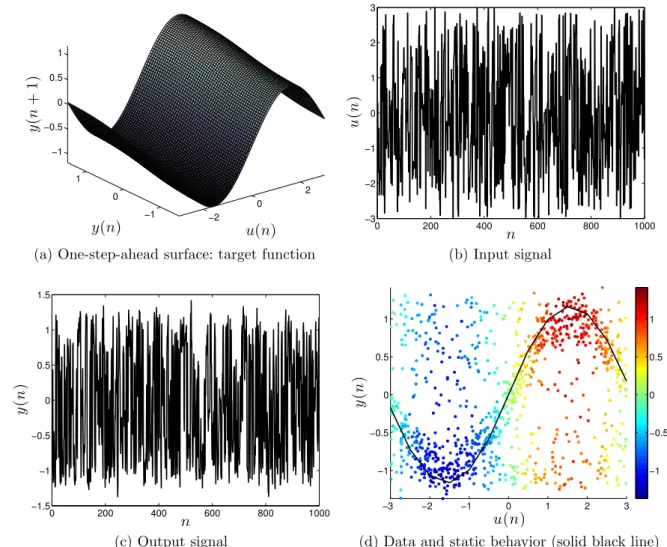
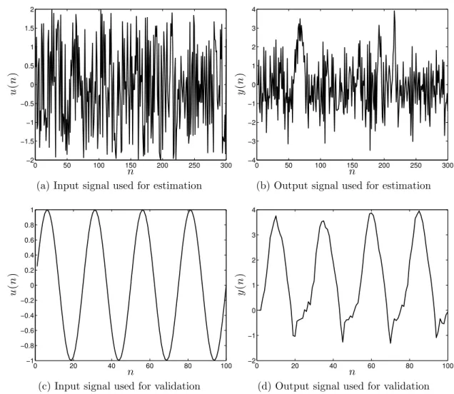
In order to illustrate the advantages and drawbacks of the methods proposed in this thesis, an artificial plant will be used repeatedly as a running example. This artificial plant has been evaluated by Gregorcic and Lightbody (2008). It consists of a discrete-time SISO system corrupted by additive noise given by
y(n+ 1) = 0.2 tanh(y(n)) + sin(u(n)) +ǫ(n). (1.9)
The artificial plant is a nonlinear dynamic system whose outputs depend on previous input and output. It corresponds to a NARX system withnu = ny = 1 and Figure 3a shows
the target function, i.e. the deterministic part of Eq. (1.9). For experimental evaluation, we generated a dataset which contains 1,000 samples with a uniformly distributed random input signal, u(n)∼ U[−3,3], and ǫ(n)∼ N(0,0.01). The input and output signals are illustrated in Figures 3b and 3c, respectively. For all experiments, we use 70% of the samples for training (model selection) and the remaining samples for testing (model validation) purposes. We have not carried out any normalization or pre-processing steps over the data samples.
Figure 3d depicts the data where colors denote the response (y(n+ 1)) along with the static equilibrium curve of the system, which represents its static behavior. To estimate the static behavior of the system, the input signal was kept constant until the convergence of the system. A set of such collections, with u(n) varying from −3 to 3, were performed and the static behavior is shown by the solid black line in Figure 3d.
Chapter 1. Introduction 24 −2 0 2 −1 0 1 −1 −0.5 0 0.5 1 u(n) y(n) y ( n + 1 )
(a) One-step-ahead surface: target function
0 200 400 600 800 1000
−3 −2 −1 0 1 2 3 n u ( n )
(b) Input signal
0 200 400 600 800 1000
−1.5 −1 −0.5 0 0.5 1 1.5 n y ( n )
(c) Output signal
−3 −2 −1 0 1 2 3
−1 −0.5 0 0.5 1 u(n) y ( n ) −1 −0.5 0 0.5 1
(d) Data and static behavior (solid black line)
Figure 3 – Artificial data created from Eq. (1.9).
✶✳✷ ❖❜❥❡❝t✐✈❡s ♦❢ t❤❡ t❤❡s✐s
The overall objective of this thesis is to propose novel approaches for nonlinear system identification using machine learning methods, which aims to produce accurate models at a low computational cost. As a consequence, we expect the novel proposals to represent feasible alternatives to classic reference methods in black-box modeling. In order to accomplish that, we shall specifically follow the next steps:
• evaluate the use of learning models based on neural networks to SISO nonlinear system identification;
• propose a novel distance-based regression approach for supervised learning and evaluate its application on system identification tasks;
• compare the different methods and paradigms on synthetic and real-world bench-marking system identification problems.
✶✳✸ ❈❤❛♣t❡r ♦r❣❛♥✐③❛t✐♦♥ ❛♥❞ ❝♦♥tr✐❜✉t✐♦♥s
In Chapter 2, global and local learning approaches that have been applied to system identification are described. It includes linear and nonlinear methods, such as a global linear method that uses ordinary least square (LS) for parameter estimation, and neural network architectures: Multilayer Perceptrons, Extreme Learning Machines and Radial Basis Functions networks. Also, a number of local approaches for system identification are discussed, such as Local Linear Regression approaches, and methods based on the Self-Organizing Map(SOM).
In Chapter 3, a novel distance-based regression method for supervised learning, called Minimal Learning Machine (MLM), is described and its application for system identification is illustrated. Original contributions of this chapter include:
• formulating a completely novel method called the Minimal Learning Machine. It includes the basic formulation and a comprehensive discussion on computational complexity and hyper-parameters.
• discussion on the links between MLM and classic methods, such as radial basis function networks;
• the proposal of supervised alternatives to the random selection of reference points in MLM.
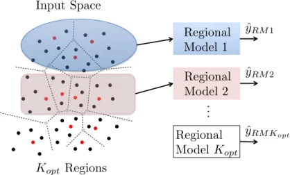
In Chapter 4, we introduce a new modeling paradigm that stands between global and local approaches and it is calledregional modeling. We describe the main characteristics of regional models and how we can use learning methods in the regional framework. Original contributions of this chapter include the following ones:
• the proposal of a new method for system identification via the clustering of the Self-Organizing Map.
• a robust extension of the proposed regional models through M-estimation (HUBER, 2004).
Chapter 1. Introduction 26
In Chapter 6, we provide concluding remarks and discuss directions for future research on topics related to this thesis.
In Appendix A, we briefly describe the clustering algorithms used in this thesis.
In Appendix B, we extend the Minimal Learning Machine to classification prob-lems, while evaluating its performance against standard classification methods. A binary classification example and four real-world problems are used for performance assessment.
In Appendix C, we evaluate the performance of the Minimal Learning Machine on eight regression problems and compare it against the state-of-the-art methods in machine learning.
✶✳✹ P✉❜❧✐❝❛t✐♦♥s
During the development of the thesis, a number of articles have been published by the author. It includes articles which relate directly to thesis topics, as well as articles related to cooperation on projects between different research groups. Despite of that, all the articles are contributions on either Machine Learning/ Computational Intelligence or System Identification areas. The published articles related to the thesis are:
1. A. H. de Souza Junior, F. Corona, G. Barreto, Y. Miche and A. Lendasse, Min-imal Learning Machine: A novel supervised distance-based method for regression and classification. Neurocomputing, to appear, 2014.
2. A. H. de Souza Junior, F. Corona and G. Barreto, Regional models: A new approach for nonlinear dynamical system identification with the Self-Organizing Map. Neurocomputing, vol. 147, n. 5, 36-45, 2015.
3. A. H. de Souza Junior, F. Corona and G. Barreto, Minimal Learning Machine and Local Linear Regression for Nonlinear System Identification. In Proc. 20th Congresso Brasileiro de Autom´atica, 2066-2073, 2014.
4. A. H. de Souza J´unior, F. Corona, Y. Miche, A. Lendasse and G. A. Barreto,
Extending the Minimal Learning Machine for Pattern Classification. In Proc. 1st BRICS Countries Congress on Computational Intelligence - BRICS-CCI 2013, 236-241, 2013.
5. A. H. de Souza J´unior, F. Corona, Y. Mich´e, A. Lendasse, G. Barreto and O. Simula,
6. F. Corona, Z. Zhu, A. H. de Souza J´unior, M. Mulas, G. A. Barreto, and R. Baratti,
Monitoring diesel fuels with Supervised Distance Preserving Projections and Local Linear Regression. InProc. 1st BRICS Countries Congress on Com-putational Intelligence - BRICS-CCI 2013, 422-427, 2013.
7. A. H. de Souza J´unior, F. Corona and G. Barreto, Robust regional modelling for nonlinear system identification using self-organising maps. InAdvances in Intelligent Systems and Computing: Advances in Self-Organizing Maps, P. A. Est´evez, J. P. Pr´ıncipe and P. Zegers Eds., vol. 198, 215-224, 2013.
8. A. H. de Souza J´unior and G. Barreto, Regional Models for Nonlinear System Identification Using the Self-Organizing Map. In Lecture Notes in Computer Science: Intelligent Data Engineering and Automated Learning - IDEAL 2012, H. Yin, J. A. F. Costa and G. A. Barreto Eds., vol. 7435, 717-724, 2012.
Also, the following papers were produced during the thesis period as a result of research collaborations:
1. F. Corona, Z. Zhu, A. H. Souza J´unior, M. Mulas, E. Muru, L. Sassu, G. Barreto, R. Baratti. Supervised Distance Preserving Projections: Applications in the quantitative analysis of diesel fuels and light cycle oils from spectra. Journal of Process Control, to appear, 2014.
2. R. L. Costalima, A. H. de Souza Junior, C. T. Souza and G. A. L. Campos,MInD: don’t use agents as objects. In Proc. 7th Conference on Artificial General Intel-ligence (Lectures Notes in Computer Science), vol. 8598, 234-237, 2014.
3. F. Corona, Z. Zhu, A. H. de Souza J´unior, M. Mulas and R. Baratti,Spectroscopic monitoring of diesel fuels using Supervised Distance Preserving Projec-tions. In Proc. IFAC 10th International Symposium on Dynamics and Control of Process Systems - DYCOPS 2013, 63-68, 2013.
4. C´esar L. C. Mattos, Amauri H. Souza J´unior, Ajalmar R. Neto, Guilherme Barreto, Ronaldo Ramos, H´elio Mazza and M´arcio Mota,A Novel Approach for Labelling Health Insurance Data for Cardiovascular Disease Risk Classification. In: 11th Brazilian Congress on Computational Intelligence, 1-6, 2013.
28
Chapter 2
Global and Local Learning Models
for System Identification
Although several techniques for nonlinear dynamic system identification have been proposed, they can be categorized into one of the two following approaches: global and local modeling. On the one hand, global modeling involves the utilization of a single model structure that approximates the whole mapping between the input and the output of the system being identified. On the other hand, local modeling utilizes multiple models to represent the input-output dynamics of the system of interest (LAWRENCE; TSOI; BACK, 1996). In this chapter we briefly overview global and local strategies for nonlinear system identification. The emphasis of this chapter is on a basic understanding of the approaches that will be further used for comparison. In Section 2.1 we discuss global models and their application to the identification of nonlinear dynamic systems. Section 2.2 introduces local modeling techniques. Section 2.3 gives the closing remarks of the chapter.
✷✳✶ ●❧♦❜❛❧ ♠♦❞❡❧✐♥❣
AMARAL, 2004) comprise classical global modeling attempts. In fact, global models constitute the mainstream in nonlinear system identification and control (YU, 2004; LI; YU, 2002; NARENDRA, 1996).
Due to the large number of global models, the focus of this thesis is on approaches from machine learning and computational intelligence fields, particularly, neural network based models. The field of machine learning abounds in efficient supervised methods and algorithms that can be equally applied to regression and classification tasks (BISHOP, 1995), and whose application in system identification is straightforward. An exhaustive and fair list of such methods would be hard to present here, but one can certainly mention as state-of-the-art methods the multilayer perceptron (MLP) (RUMELHART; HINTON; WILLIAMS, 1986), radial basis functions networks (RBF) (POGGIO; GIROSI, 1990; WU et al., 2012) support vector regression (SVR) (VAPNIK, 1998; SMOLA; SCHOLKOPF, 2004), as well as more recent approaches, such as those based on extreme learning machine (ELM) (HUANG; ZHU; ZIEW, 2006), Gaussian processes (RASMUSSEN; WILLIAMS,
2006) and information-theoretic learning(ITL) (PRINCIPE, 2010).
This section describes global approaches for nonlinear system identification, includ-ing the well-known ordinary least square (LS) estimation method, which is commonly used for estimating part of the nonlinear model’s parameters. In Section 2.1.2, we briefly report neural network architectures and their application to system identification.
✷✳✶✳✶ ▲❡❛st ❙q✉❛r❡s ❛♥❞ ❆❘❳ ♠♦❞❡❧s
As previously mentioned, the ordinary least squares method (RAO; TOUTEN-BURG, 1999) is an estimation method applied to linear-in-the-parameter models. Despite its early proposal, it is still one of the most used methods in machine learning and related areas.
We are interested in approximating a target function f : X→ Y from empirical input and output observations {(xn, yn)}Nn=1, with xn ∈ RD and yn ∈ R, following the
model in Eq. (1.1). For this task, one can use the linear model/hypothesis
h(x) =βTx, (2.1)
where h : RD → R, β = {β
j}Dj=1 is the vector of parameters and x = {xj}Dj=1 is the
regression vector (or regressors).
As usual, we need to quantify how wellh approximates f. A reasonable choice to ensure approximation quality is the squared error e(f(x), h(x)) = (h(x)−f(x))2, which
can be summed over the whole set of observations: PNn=1(h(xn)−f(xn))2. Unfortunately,
Chapter 2. Global and Local Learning Models for System Identification 30
approximation to f. In doing so, we define the least square loss function JLS by
JLS(β) = N X
n=1
(h(xn)−yn)2, (2.2)
By minimizing (2.2) using the model (2.1), we have that the least squares estimator is
ˆ
β= XTX−1XTy. (2.3)
where the matrix X= [x1,x2, . . .xN]T is an N×D matrix whosen-th row corresponds to
the n-th regression vector xT
n. Similarly, the column vector y encompasses the N output
observations in its rows.
We may assume that the dynamic SISO system we are working with can be described mathematically by the ARX (AutoRegressive with eXogenous input) model (LJUNG, 1999):
y(n) = a1y(n−1) +· · ·+anyy(n−ny) +b1u(n−n0−1) +· · ·+bnuu(n−n0−nu) +ǫ(n),
=
ny X
j=1
ajy(n−j) + nu X
l=1
blu(n−n0−l) +ǫ(n), (2.4)
where u(n)∈Rand y(n)∈R denote, respectively, the input and output of the model at time step n, while nu ≥1 and ny ≥1 are the input-memory and output-memory orders,
respectively. The error termǫ(n) is assumed to follow a white noise process. The parameter
n0 (n0 ≥0) is a delay term, known as the process dead-time. Without lack of generality,
we assumen0 = 0 in this thesis, thus obtaining the following ARX model:
y(n) =
ny X
j=1
ajy(n−j) + nu X
l=1
blu(n−l) +ǫ(n). (2.5)
By defining the input vector x(n) ∈ Rnu+ny at time step n and the vector of parameters β ∈Rnu+ny as
x(n) = [y(n−1) · · · y(n−ny)|u(n−1) · · · u(n−nu)]T, (2.6) β = [a1 · · · any |b1 · · · bnu]T, (2.7)
we can write the output of the ARX model in Eq. (2.5) simply as
y(n) = βTx(n) +ǫ(n) (2.8)
with ˆβgiven by Eq. (2.3). Under the assumption that ǫ(n) is white noise, the LS estimator is unbiased and equivalent to the maximum likelihood estimator (AGUIRRE, 2007).
Since the LS estimation solution will be used extensively throughout the thesis, important remarks are necessary. An important issue is that the regression matrix X must be full-rank. Otherwise, XTX does not have an inverse. Also, the number of rows N of X
must exceed (or equal) the number of columns D in Eq. (2.3). If not, XTXis not full-rank
and it may not correspond to the LS estimator. In those cases where N < D, a least-norm solution is usually preferred and it represents a regularized solution. Clearly, situations in which N < D are undesired for estimation and data fitting purposes since an infinity number of solutions is possible. From now on, in the context of system identification,
D=ny+nu.
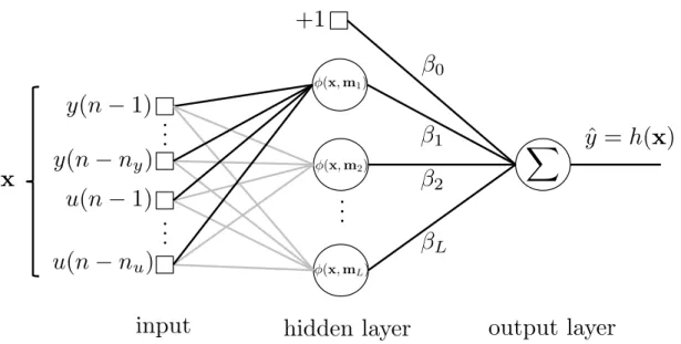
✷✳✶✳✷ ❙✐♥❣❧❡✲❤✐❞❞❡♥ ❧❛②❡r ❢❡❡❞❢♦r✇❛r❞ ♥❡t✇♦r❦s
In this section, we briefly discussartificial neural networks (ANN), specifically a special type of ANN called single-hidden layer feedforward networks (SLFN). The term “artificial neural networks” was originally motivated by the way that biological structures process information in the brains of humans and other animals. However, eventually, most artificial neural networks used in engineering are at least as closely related to mathematics, statistics and optimization as to the biological model (NELLES, 2001). ANNs are based on processing units called neurons or nodes which are combined to form a network. An SLFN has one hidden layer of neurons that work in parallel. These neurons are connected to other neurons in the output layer. The layers may be organized in such a way that the input vector enters the hidden layer and then reaches the output layer. The mathematical representation of SLFN is given by
h(x) =
L X
l=1
βlφ(x,ml) +β0 =βTz, (2.9)
whereL denotes the number of neurons in the hidden layer, β∈RL+1 is the weight vector
of the linear output unit, φ(·) : R → R is a nonlinear mapping, also called activation function, which depends on the input vector x∈Rny+nu and the vector of parameters ml
of the l-th hidden unit. The notation φ(x,ml) stands for the fact that the fixed univariate
mapping φ(·) depends on the input vector and the parameters of the hidden units, and we can simplify the notation by expressing φ(x,ml) =φl(x). An alternative interpretation
for Eq. (2.9) is that the vector z results of a nonlinear transform Φ : X→ Z on x such that z= [1, φ1(x), . . . , φL(x)]T. Thus, we can write z= Φ(x). In other words, the SLFN
Chapter 2. Global and Local Learning Models for System Identification 32
y
(
n
−
1)
y
(
n
−
n
y)..
.
..
.
u
(
n
−
1)
u
(
n
−
n
u)x
..
.
input
hidden layer
output layer
ˆ
y
=
h(x)
+1
�
φ(x,m1)
φ(x,m2)
φ(x,mL)
β
0β
1β
Lβ
2Figure 4 – General structure of single-hidden layer feedforward networks.
The SLFN approaches differ in the way they define φ(·) and the parameters ml,
how they combine x and ml to provide a single variable as input for φ, and how they
compute β. In the following, we present the particularities of the Radial Basis Functions Networks, Multilayer Perceptrons and Extreme Learning Machines. For an overview of most neural network architectures, we recommend Haykin (2009). Bishop (2006) discusses the use of neural networks for pattern classification, including Bayesian approaches. For a review of neural networks for system identification, we suggest the books by Nelles (2001) and Norgaard et al. (2000), and the seminal paper by Narendra and Parthasarathy (1990).
✷✳✶✳✷✳✶ ▼✉❧t✐▲❛②❡r P❡r❝❡♣tr♦♥s
Themultilayer perceptrons (MLP) (HAYKIN, 2009) is the most widely known and used neural network architecture. In the literature, the MLP is even used as a synonym for neural networks. The operation of MLPs is based on units or neurons called perceptrons. The operation of these neurons can be split into two parts. The first part consists of projecting the input vector xon the weights ml through the inner product mTl x. Second,
the nonlinear activation function φ transforms the projection result. If several perceptron neurons are used in parallel and connected to an output neuron, the MLP network with one hidden layer is obtained. The MLP can be mathematically formulated as
h(x) =
L X
l=1
βlφ(mTl x) +β0 =βTz, (2.10)
where Lis the number of hidden neurons, x∈Rny+nu+1 is the input vector added a bias term x0 = 1, ml ∈ Rny+nu+1 is the weight vector of the l-th hidden neuron, β ∈ RL+1
is the weight vector of the output unit and, z = [1, φ(mT
1x), . . . , φ(mTLx)]T represents
the projection of x in the space of the hidden layer. Common choices for the activation function φ(·) :R→Rare the logistic function φ(mT
tangentφ(mT
l x) = tanh(mTl x). The two functions share the interesting property that their
derivative can be expressed in terms of the function itself (NELLES, 2001).
The estimation of the parameters of an MLP, e.g.βand{ml}Ll=1, is usually achieved
by minimizing the difference between the network output h(x(n)) and the measured output
y(n) from the estimation samples {(x(n), y(n))}N
n=1. The typical approach to MLP training
is the error back-propagation algorithm (RUMELHART; HINTON; WILLIAMS, 1986). Essentially, this procedure applies chain rule for derivative calculations with respect to the parameters, which corresponds to a steepest descent algorithm. In fact, many nonlinear optimization techniques can be used to estimate the MLP parameters. A description of strategies for MLP training is beyond the scope of this thesis, and can be found in Haykin (2009), Nelles (2001) and Bishop (1995).
The MLP network, as described by Eq. (2.10), represents only the most commonly applied MLP type. Different variants exist. Sometimes the output neuron is not of the pure linear combination type but is chosen as a complete perceptron. This means that an additional activation function at the output is used. Another possible extension is the use of more than one hidden layer. In fact, it can be used as many hidden layer as necessary. SLFNs with several hidden layers have gained special attention from the machine learning community recently, under the general name of deep networks, since efficient learning algorithms for training such networks have been derived (BENGIO, 2009).
✷✳✶✳✷✳✷ ❊①tr❡♠❡ ▲❡❛r♥✐♥❣ ▼❛❝❤✐♥❡s
The Extreme Learning Machine (ELM) is a class of SLFNs, recently proposed by Huang, Zhu and Ziew (2006), for which the weights from the inputs to the hidden neurons are randomly chosen, while only the weights from the hidden neurons to the output are analytically estimated. The hidden layer does not need to be tuned, and its parameters are independent of training data. According to Huang, Wang and Lan (2011), ELM offers significant advantages, such as a fast learning speed, ease of implementation, and less human intervention than more traditional SLFNs, such as the MLP network.
In general, the structure of ELM is the same as MLP, including the choice for the activation function φ. The difference between MLP and ELM relies on the learning algorithm, i.e., how the model parameters are estimated. Whereas the MLP is usually trained using nonlinear optimization techniques, the ELM training consists of two steps:
1. Random initialization of the weights in the hidden layer{ml}Ll=1. Usually, the weight
vectorsml are randomly sampled from a uniform (or normal) distribution.
2. Estimation of the output weights by the LS algorithm.
Chapter 2. Global and Local Learning Models for System Identification 34
N ×(L+ 1) matrix whose N rows are the hidden-layer output vectors z(n) ∈ RL+1,
n = 1, ..., N, where N is the number of available training input patterns, and z(n) = [1, φ(mT
1x(n)), . . . , φ(mTLx(n))]T. Similarly, let y = [y(1) y(2) · · · y(N)]T be a N ×1
vector whose then-th row is the output observationy(n) associated with the input pattern
x(n). Since the ELM is linear in the parameters β, the weight vector β can be easily computed by means of the LS method as follows
ˆ
β= ZTZ−1ZTy. (2.11)
✷✳✶✳✷✳✸ ❘❛❞✐❛❧ ❇❛s✐s ❋✉♥❝t✐♦♥ ◆❡t✇♦r❦s
TheRadial Basis Function network (RBF) (BUHMANN, 2003) is also an SLFN, with the difference being that the activation function φ, also called radial basis function, depends on a distance metric. A radial basis function approximation of a function f :
Rny+nu →R takes the form
h(x) =
L X
l=1
βlφ(kx−mlk2) +β0, (2.12)
where φ : [0,∞) → R is a fixed univariate function, β = [β0, β1, β2, . . . , βL]T denotes a
vector of coefficients usually estimated by the LS method andml ∈Rny+nu corresponds to
the centers of the radial basis functions φ(.). In other words, the RBF approximation is a linear combination of translates of a fixed function φ(·) of a single real variable. In system identification applications, it is common to add an autoregressive and moving average linear terms to Eq. (2.12) (ALVES; CORREA; AGUIRRE, 2007).
Historically, radial basis functions were introduced in the context of exact function interpolation. Thus, usually the number of centers equals the number of learning points,
L= N, and the centers are the learning points, mn =x(n), forn = 1, . . . , N. In this case,
the RBF approximation (Eq. 2.12) may fit the training examples perfectly. However, in machine learning applications, the output observations are noisy, and exact interpolation is undesirable because it may lead to overfitting.
The design of RBF models encompasses four basic decisions:i) The choice of radial basis functions φ(·); ii) How to compute the coefficients{βl}Ll=0;iii) How to determine the
number of radial basis function L; and iv) How to locate the centers ml and dispersion σl.
Among a variety of radial basis functions, some well-known functions are listed below:
• Linear: φ(kx−mlk) = kx−mlk.
• Cubic: φ(kx−mlk) = kx−mlk3.
• Multiquadric: φ(kx−mlk) = p
• Gaussian: φ(kx−mlk) = exp
−kx−mlk2
σ2
l
, whereσl ∈R is a constant.
The coefficients of the linear output unitβ are generally computed using the LS algorithm. In doing so, let us define the matrix Z={znl}, withzn0 = 1 for alln= 1, . . . , N,
and
znl =φ(kx(n)−mlk), n = 1, . . . , N;l = 1, . . . , L.
where N again represents the number of training points. In addition, let us collect the output observations y(n),n = 1, . . . , N in a column vector y. Thus, the LS estimation of
β ∈RL+1 is
ˆ
β= ZTZ−1ZTy. (2.13)
The number of radial basis function L, as well as the hyper-parameters σl, are
usually optimized using sampling methods, like k-fold cross-validation. Regarding the choice of the centers of the radial basis functions ml, many approaches are feasible.
The simplest strategy would be to select the center randomly from the training points
{x(n)}. Another possibility is through clustering on the input space, which constitutes the standard approach. Normally, the k-means algorithm (MACQUEEN, 1967) is used to provide prototypes as centers of the radial functions. The drawback of these methods is that the center location depends only on training data distribution in the input space. Thus, the complexity of the underlying function that has to be approximated is not taken into account. Supervised techniques that use output information to locate the centers where the underlying function to be approximated is more complex are usually desired. An efficient supervised learning approach for choosing centers is proposed by Chen, Cowan and Grant (1991). For an overview of different strategies for center placement in RBF networks, we recommend Sarra and Kansa (2009) and Nelles (2001).
✷✳✷ ▲♦❝❛❧ ♠♦❞❡❧✐♥❣
Local modeling consists in a divide-and-conquer approach where the function approximation problem is solved by dividing it into simpler problems whose solutions can be combined to yield a solution to the original problem. These approaches have been a source of much interest because they have the ability to locally fit the shape of an arbitrary surface. This feature is particularly important when the dynamic system characteristics vary considerably throughout the input space. Regarding learning models, there are two main different local modeling approaches: i) modular architectures, and
Chapter 2. Global and Local Learning Models for System Identification 36
Model Network (LMN) (MURRAY-SMITH, 1994; HAMETNER; JAKUBEK, 2013), the Local Linear Mapping (LLM) (WALTER; RITTER; SCHULTEN, 1990), the Adaptive-Network-Based Fuzzy Inference System (ANFIS) (JANG, 1993), Takagi-Sugeno (TS) models (TAKAGI; SUGENO, 1985), and Mixture of Experts (MEs) (JACOBS et al., 1991; LIMA; COELHO; VON ZUBEN, 2007).
Local Model 1
Local Model 2
Local
Model Q
.. . Input Space
Q Partitions
ˆ yLM1
ˆ yLM2
ˆ yLM Q
Figure 5 – Illustration of a local modeling approach: modular architectures.
Local approximating approaches turn the problem of function estimation into a problem of value estimation. In other words, they do not aim to return a complete description of the input/output mapping but rather to approximate the function in a neighborhood of the point to be predicted. Examples of local approximating methods are Lazy Learning (LL) (BONTEMPI; BIRATTARI; BERSINI, 1999), Locally Weighted Learning (LWL) (ATKESON; MOORE; SCHAAL, 1997), Local Linear Regression (LLR) (GUPTA; GARCIA; CHIN, 2008), and the kSOM model (SOUZA; BARRETO, 2010).
MEs ANFIS
LMN
LLM
LL LWL
kSOM
LLR TS
Divide-Conquer Approaches
SOM-based Fuzzy Inference
Figure 6 – Taxonomy of divide-and-conquer approaches. Blue circles denote local approxi-mating methods whereas green circles represent modular architectures.
to represent a comprehensive list of methods. In what follows, we discuss local modeling approaches, including both modular architectures and local approximating strategies.
✷✳✷✳✶ ▼♦❞✉❧❛r ❛r❝❤✐t❡❝t✉r❡s
In this section, we describe classic modular approaches to the system identification problem. We focus on methods based on the Self-Organizing Map (SOM) (KOHONEN, 2013). First, we briefly introduce the Self-Organizing Map algorithm. Second, we explore an alternative for using the Self-Organizing Map to build regression models for system identification, the Local Linear Map (LLM) model.
✷✳✷✳✶✳✶ ❚❤❡ ❙❡❧❢✲❖r❣❛♥✐③✐♥❣ ▼❛♣
TheSelf-Organizing Mapis a well-known competitive learning algorithm. The SOM learns from examples a mapping (projection) from a high-dimensional continuous input space Xonto a low-dimensional discrete space (lattice)AofQneurons, which are arranged in fixed topological forms, e.g., as a rectangular 2-dimensional array. The mapi∗(x) : X→A,
defined by the set of prototypes or weight vectors W = {w1,w2, . . . ,wQ},wi ∈ Rnu+ny,
assigns to an input vector x∈Rnu+ny awinning neuron i∗ ∈A, determined by
i∗ = arg min
∀i kx−wik, (2.14)
wherek · k denotes the Euclidean distance.
During SOM iterative training, at each training step j, one sample vector x(n(j)) is randomly chosen from the input data set X. The winning neuron and its topological neighbors are moved closer to the input vector by the following weight update rule:
wi(j+ 1) =wi(j) +α(j)η(i∗, i;j)[x(n(j))−wi(j)] (2.15)
where 0< α(j)<1 is the learning rate and η(i∗, i;j) is a weighting function which limits
the neighborhood of the winning neuron. A usual choice for η(i∗, i;j) is given by the
Gaussian function:
η(i∗, i;j) = exp
−ki(j)−i
∗(j)k2
2σ2(j)
(2.16)
where i(j) and i∗(j) are respectively, the coordinates of the neuronsi and i∗ in the output
array at time j, and σ(j)>0 defines the radius of the neighborhood function at time j. The variablesα(j) and σ(j) should both decay with time to guarantee convergence of the weight vectors to stable steady states. In this thesis, we adopt an exponential decay for both variables α(j) and σ(j).
Chapter 2. Global and Local Learning Models for System Identification 38
are mapped into adjacent regions on the map. Due to this topology-preserving property, the SOM is able to cluster input information and spatial relationships of the data on the map. Despite its simplicity, the SOM algorithm has been applied to a variety of complex problems (VAN HULLE, 2010; YIN, 2008; KOHONEN et al., 1996) and has become one of the most popular artificial neural networks.
✷✳✷✳✶✳✷ ❚❤❡ ▲♦❝❛❧ ▲✐♥❡❛r ▼❛♣
The first local modeling approach to be described has been calledLocal Linear Map (LLM) (WALTER; RITTER; SCHULTEN, 1990) by its proponents, and was originally applied to nonlinear time series prediction. The basic idea of the LLM is to associate each neuron in the SOM with a linear finite impulse response (FIR) filter trained with the least mean squares (LMS) adaptation algorithm (WIDROW, 2005). The SOM array is used to quantize the input space in a reduced number of prototype vectors (hence, Voronoi regions), while the filter associated with the winning neuron provides a local linear estimate of the output of the mapping being approximated.
For modeling purposes, the input vectorx(n) is built at each time stepn by sliding through the input-output time series. Vector quantization of the input spaceXis performed by the LLM as in the usual SOM algorithm, with each neuron i owning a prototype vector
wi, i= 1, . . . , Q. In addition, associated with each weight vectorwi, there is a coefficient
vector βi ∈Rnu+ny of the i-th local model.
The output value of the LLM-based local model is computed as
ˆ
y=βiT∗x, (2.17)
where βi∗ is the coefficient vector associated with the winning neuron i∗ for x. From
Eq. (2.17), one can easily note that the coefficient vector βi∗ is used to build a local linear
approximation of the unknown global input-output mapping or target function.
Since the adjustable parameters of the LLM algorithm are the set of prototype vectorswi and their associated coefficient vectors βi, i= 1,2, . . . , Q, we need two learning
rules. The rule for updating the prototype vectors wi follows exactly the one given in
Eq. (2.15). The learning rule of the coefficient vectorsβi(j) is an extension of the normalized
LMS algorithm, that also takes into account the influence of the neighborhood function
η(i∗, i;j):
βi(j+ 1) =βi(j) +α′(j)η(i∗, i;j)∆βi(j), (2.18) where 0< α′(j)<1 denotes the learning rate of the coefficient vector, and ∆β
i(j) is the
error correction rule of Widrow-Hoff, given by
∆βi(j) =
y(n(j))−βiT(j)x(n(j)) x(n(j))
where x(n(j)) and y(n(j)) are randomly chosen input sample and corresponding output from the training sets X andY. After trained for a large number of iterations, the weight vectors wi(j) of the SOM and the associated coefficient vectors βi(j) are “frozen”.
The basic idea behind the SOM-based local approaches is the partitioning of the input space into non-overlapping regions, called Voronoi cells, whose centroids correspond to the weight vectors of the SOM. Then an interpolating hyperplane is associated with each Voronoi cell or a small subset of them, in order to estimate the output value of the target function.
✷✳✷✳✷ ▲♦❝❛❧ ❛♣♣r♦①✐♠❛t✐♥❣ ♠♦❞❡❧s
Local approximating strategies have been proposed in the literature of system identification and machine learning under many different names, such as just-in-time models, prototype-based or memory-based methods, lazy learning, and look-up tables. In this section, we focus on the SOM-based approaches and we discuss the recently proposed local linear regression methods with enclosing neighborhood.
✷✳✷✳✷✳✶ ❚❤❡ ❱◗❚❆▼ ❆♣♣r♦❛❝❤
The Vector-Quantized Temporal Associative Memory (VQTAM) (BARRETO; ARA´UJO, 2004) approach aims to build an input-output associative mapping using the Self-Organizing Map. It is a generalization to the temporal domain of a SOM-based asso-ciative memory technique that has been used by many authors to learn static (memoryless) input-output mappings, especially within the domain of robotics.
According to the VQTAM framework for system identification, during the training process, the training set X has its elements x(n) augmented by incorporating output information y(n). In doing so, the augmented input vector xaug(n)∈Rnu+ny+1 is given by
xaug(n) = [x(n), y(n)] = [y(n−1), . . . , y(n−ny), u(n−1), . . . , u(n−nu), y(n)].
As expected, the augmented prototypes of the SOM networkwaugi ∈Rnu+ny+1 can be decomposed into two parts as well. The first part, denoted by wi ∈ Rny+nu, carries
information about the original input space. The second part, denoted wouti ∈R, represents
the coordinate associated with output information, such that waugi = [wi, wouti ].
The VQTAM learning algorithm differs slightly from the basic SOM algorithm. The winning neuron is determined based only on the original input space, such that
i∗ = argmin
∀i∈A {k
x−wik}. (2.20)
In the iterative weight updating step, the augmented vectors are used: