3D CATENARY CURVE FITTING FOR GEOMETRIC CALIBRATION
Ting On Chan and Derek D. Lichti
Department of Geomatics Engineering, University of Calgary
2500 University Dr NW, Calgary, Alberta, T2N1N4 Canada
(ting.chan, ddlichti)@ucalgary.ca
Commission V, WG V/3
KEY WORDS: 3D catenary model, least square fitting, parameter correlation, hanging power cables ABSTRACT:
In modern road surveys, hanging power cables are among the most commonly found geometric features. These cables are catenary curves that are conventionally modelled with three parameters in 2D Cartesian space. With the advent and popularity of the mobile mapping system (MMS), the 3D point clouds of hanging power cables can be captured within a short period of time. These point clouds, similarly to those of planar features, can be used for feature based self calibration of the system assembly errors of an MMS. However, to achieve this, a well defined 3D equation for the catenary curve is needed. This paper proposes three 3D catenary curve models, each having different parameters. The models are examined by least squares fitting of simulated data and real data captured with an MMS. The outcome of the fitting is investigated in terms of the residuals and correlation matrices. Among the proposed models, one of them could estimate the parameters accurately and without any extreme correlation between the variables. This model can also be applied to those transmission lines captured by airborne laser scanning or any other hanging cable like objects.
1. INTRODUCTION
Hanging power cables (Figure 1) are very commonly found geometric features in modern cities. A hanging power cable is in a chain structure loaded only by its own weight and therefore its 3D shape can be classified as a catenary feature. These features have been investigated intensively in terms of their 3D point clouds captured with airborne LiDAR and mobile mapping systems (MMSs) for various applications by a number of researchers. Some examples include: the detection and segmentation of transmission lines using airborne LiDAR data (Mclaughlin 2006); the reconstruction of transmission lines with airborne LiDAR data by Jwa and Sohn (2009); the estimation of the height of hanging cables for road safety purposes with the StreetMapper system developed by Kremer and Hunter (2007); and the assessment of LiDAR accuracy of the Optech System using transmission wires (Ussyshkin and Smith 2007).
Figure 1. Hanging power cables in a road corridor in Canada
Among the above applications, Ussyshkin and Smith (2007), for instance, modelled the transmission lines with a two step process. In the first step, the azimuth of the power line was determined by fitting a straight line to the x and y coordinates. Then, the transformed x and the z coordinates were used to solve the conventional 2D equation of the catenary curve. Jwa
and Sohn (2009) first estimated the orientation of the transmission lines using the 2D line equation augmented with θ and ρ, followed by the reconstruction based on the 2D catenary model. In both cases, the 3D modelling process was broken down into two 2D processes. Whilst sufficient for the respective applications, such an approach is not as geometrically rigorous as a 3D model that considers the geometric contribution of x, y, and z simultaneously.
As a result, a 3D catenary equation is desired, particularly for geometric calibration of the boresight parameters of an MMS. This paper formulates three different mathematical models for a 3D catenary curve for conditioning the points lying on the curve during a least square adjustment of calibration. Similar ideas using planar features for calibration have been successfully implemented for airborne systems (Skaloud and Lichti 2006) and also the MMSs (Glennie and Lichti 2010; Rieger et al 2010). With a 3D equation, the catenary curves can serve as extra conditions in addition to the planar features used in the calibration.
2. 2D CATENARY MODEL
The most basic form of the 2D catenary curve can be expressed with the following equation (Lockwood 1961):
⋅
c
x
cosh
c
=
y
(1)where c is a scaling factor that is governed by the ratio between the tension at the cable’s vertices and the weight of the cable per unit length. Equation 1 can be further extended to include two translation parameters (a and b) as given in the following equation (Levinson and Kane 1993):
⋅
+
c
b
x
cosh
c
a
=
y
(2)where a and b are the translation parameters from the origin along the y and x axis respectively.
When Equation 2 is used to model a catenary curve in 3D space, the following two equations can be used:
⋅
+
1 1 1
1
c
b
x
cosh
c
a
=
z
(3)
⋅
+
2 2 2
2
c
b
y
cosh
c
a
=
z
(4)Figure 2 shows that the point cloud of a real hanging power cable in catenary shape can be viewed in either z x plane or z y plane. For more about the catenary and its history, please see Chatterjee and Nita (2010).
Figure 2. Real catenary point cloud (x y z, z x, z y)
3. THE AZIMUTH AND DISTANCE FROM THE ORIGIN OF THE CATENARY
The projection of a 3D catenary onto the x y plane should be a straight line. Instead of using the slope and y intercept, the azimuth (θ) and distance from the origin (ρ) can be used to parameterize the straight line. In this section, the relation between the catenary curve parameters (a, b, c), θ and ρ is investigated prior to the formulation of the 3D catenary models. Figure 3 illustrates the relationship between θ and ρ, and the position of two catenary curves in the x y plane.
Figure 3. Catenary positions with θ and ρ
Figure 4. Simulated catenary curves (x y z)
Figure 5. Simulated catenary curves (x y)
The geometric relationships between the two sets of parameters of Equations 3 and 4 (total of six parameters: a1, b1, c1; a2, b2,
c2) with θ and ρ were examined with 30 simulated 3D catenary
curves (Figures 4 and 5). The first six catenary curves are parallel to the x axis and symmetric around the y axis. The distance between any two of the catenary curves is constant. Their azimuths are 0˚. The remaining 24 catenaries were generated by rotating the first 6 catenaries by 30˚, 45˚, 60˚ and 90˚.
Equations 3 and 4 were then used as the models for least squares fitting to estimate the parameters. Table 1 shows that parameters estimation results of the first catenary curve (marked with * in Figure 5) and its rotated conjugates. The two sets of parameters (a1, b1, c1; a2, b2, c2) vary in a very systematic
manner as a function of the rotation angle θ. When θ equals 45˚, the two sets of parameters are equal to each other. All six parameters are functions of θ.
Table 1. Parameters of the first catenary curve (marked with * in Figure 5)
a1 b1 c1 a2 b2 c2
0˚ 20.0 0 100
30˚ 43.2 1062.5 77 91.2 1840.3 29.6
45˚ 66.7 1502.6 53.7 66.7 1502.6 53.7
60˚ 91.2 1840.3 29.6 43.2 1062.5 77
90˚ 20 0 100
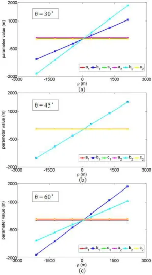
When θ is constant, the a1, a2, c1and c2 parameters will remain
constant as ρ varies as shown in Figure 6. When θ equals 30˚, the slope of b1 is less than that of b2, but this is opposite when θ
equals 60˚. When θ equals 45˚, b1 and b2 are equivalent. In fact,
only the b parameter will vary when a catenary is translated in
the direction of its orientation. However, all three parameters will vary if the catenary is translated in other directions.
Figure 6. Values of a1, b1, c1; a2, b2, c2 vs ρ for constant θ
4. PROPOSED MODELS
In this section, the following three 3D mathematical models for the catenary are presented and will be evaluated in the next section:
• Model with a, b, c and θ • Model with a, c, θ and ρ
• Model with a, b, c and centroid of (x,y) 4.1 Model 1: a, b, c and θ
This model comprises four parameters: a, b, c and θ. First, a new x coordinate is defined by the clock wise rotation of the original xy coordinates (Equation 5).
θ
θ
θ
−
θ
=
′
′
y
x
cos
sin
sin
cos
y
x
(5)This relationship is then substituted into Equation 3, we have:
−
θ
−
θ
⋅
+
1
c
b
sin
y
xcos
cosh
c
a
=
z
(6)The subtraction of 1 from the hyperbolic cosine term was employed by Sugden (1994). Subsequent evaluation testing has shown that this measure helps de correlate a from the other model parameters.
4.2 Model 2: a, c, θ and ρ
Figure 7 shows the relationship between b1, b2, θ and ρ. In order
to reduce the correlation between b and other model variables, the b term can be replaced by ρsinθ, which still leaves four parameters in comparison to Equation 6. The model is given as:
−
θ
−
θ
ρ
θ
⋅
+
1
c
sin
sin
y
xcos
cosh
c
a
=
z
(7)Figure 7. Relationship between b1, b2, θ and ρ
4.3 Model 3: a, b, c and centroid of (x,y)
In Section 3, it was shown that a, b and c are functions of θ and that b is a function of ρ. Thus, θ and ρ can be eliminated. In this model, the catenary orientation implicitly modelled with the distance, u, from the centroid of the xy coordiantes of the set of points on the curve. It is known from regression that the centroid position lies on the best fit straight line. The centroid, (xm, ym) is not estimated in the least squares process, but is
updated in each iteration as the observations are updated in the Gauss Helmert adjustment model.
−
−
⋅
+
1
c
b
u
cosh
c
a
=
z
(8)(
) (
)
2m 2
m
y
y
x
x
=
u
±
−
+
−
(9)5. MODELS EVALUATION RESULTS
5.1 Model Evaluation with Simulated Data
First, a noise free, symmetric catenary with 25 points and parameters (a1=43.2 m, b1=1062.5 m, c1=77.1 m, θ =30˚ and ρ =
2125 m) was simulated to evaluate each of the models. Each of the three models was able to estimate the parameters accurately, but with different degrees of correlation between the parameters. The z residuals of the three models proposed are shown in Figure 8. The z residuals of Model 3 are higher than the other two models but their magnitudes are still insignificant (in order of 1012), which, indicates the model fitting is
appropriate. Therefore, Model 1, 2 and 3 are effectively the same in terms of fit.
Figure 8. z residuals from the 3D catenary model least squares fitting with the simulated data.
5.1.1 Model 1: a, b, c and θ
Table 2 shows that b, c and θ are very highly correlated with each other. This is an expected outcome given the results from Section 3, i.e. the a, b and c parameters are functions of θ and therefore they are expected to have very high correlations.
Table 2. Correlation coefficients of Model 1: a, b, c and θ
a b c θ
a 1 0.59 0.58 0.59
b 0.59 1 0.99 0.99
c 0.58 0.99 1 0.99
θ 0.59 0.99 0.99 1
5.1.2 Model 2: a, c, θ and ρ
The objective of replacing b with θ and ρ is to determine whether the high correlation that exists between b and the other parameters can be removed. From Table 3, it can be seen that this measure was only partly successful. High correlation still exists between c and θ even though ρ is not correlated with other parameters.
Table 3. Correlation coefficients of Model 2
a c ρ θ
a 1 0.59 0 0.6
c 0.58 1 0 0.99
ρ 0 0 1 0
θ 0.6 0.99 0 1
5.1.3 Model 3: a, b, c and centroid of (x,y)
Table 4 gives the correlation coefficients of the simulated curves shown in Figure 9. Clearly, no extreme correlations among the parameters exist when the catenary is symmetric. In order to aid the interpretation of the results, the normalized height difference between the two ends of the catenary is defined as:
L H =
Hn (10)
where L is the length of the catenary projected onto the horizontal plane and IH is the height difference between the two ends of the catenary.
Table 4. Correlation coefficients of Model 3
a b c a b c
a 1 0 0.74 1 0.15 0.73
b 0 1 0 0.15 1 0.35
c 0.74 0 1 0.73 0.35 1
a 1 0.2 0.59 1 0.3 0.02
b 0.2 1 0.75 0.3 1 0.91
c 0.59 0.75 1 0.02 0.91 1
Catenary in Figure 9(a) Catenary in Figure 9(b)
Catenary in Figure 9(c) Catenary in Figure 9(d)
Figure 9. Height difference and symmetry of the catenary curve
The correlation between the b and c parameters is a function of both IHn and L. It can be seen in Figure 10 that as IHn
increases, the correlation between b and c increases (as does the catenary asymmetry). However, increasing L has the effect of lowering the correlation.
Figure 10. Correlation coefficient of b and c vs. ΔHn
5.2 Model Evaluation with Real Data
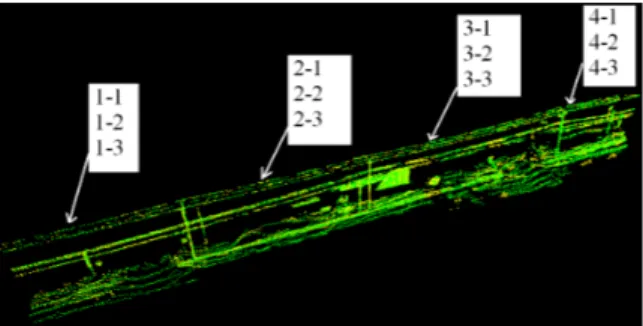
Model 3 (a, b, c, xm and ym) has been evaluated with real data.
Twelve hanging power cables (4 sets of cables; 3 nearly parallel catenary curves in each set) have been manually extracted from a point cloud captured with the TITAN System developed by Terrapoint Inc. (Figure 11).
Figure 11. Hanging power cables point cloud for testing the model
The data was collected in an urban area of Montreal, Canada in 2008. The data density is 1000 – 8000 points/m2. For more
about the TITAN, please see Glennie (2009). The estimated paramters are summarized in Table 5.
Table 5: Estimated parameters of Model 3 from the real power cables point cloud dataset.
a b c a b c
1?1 8.6 0.9 516.3 2?1 8.6 2.5 489.3
1?2 8.6 1 344.7 2?2 8.4 2.5 379.7
1?3 8.6 0.7 385.9 2?3 8.4 1.6 438.4
3?1 9.1 3.1 468.5 4?1 7.8 13.2 435.4
3?2 9.1 0.9 371.9 4?2 7.7 10.6 412.1
3?3 8.9 2.7 332.3 4?3 7.6 15.5 485.3
All the twelve catenary curves (hanging power cables) have distinguishable estimated parameters. The high correlation between b and c of catenary 4 1 (Table 6) exists because this cable (as well as 4 2 and 4 3) all are extremely asymmetric. The height difference between two ends (IH) is approximately 1.3 m and the length of the curve projected on the horizontal plane (L) is approximately 38 m (IHn = 0.034). This result is
consistent with the high correlation values of the simulated data (the red curve of Figure 10). Therefore, depending on L, the degree of symmetry has to be considered seriously and extremely asymmetric catenary curves should not be used. The z residuals of the four hanging power cables are shown in Figure 12.
Figure 12. Residuals of the least square fitting of the real power cable point cloud using Model 3
No systematic trends are apparent in the z residuals (Figure 12) from any of the four catenary fits using Model 3, regardless of asymmetry, including curve 4 1. This suggests along with the simulation results that Model 3 is indeed a valid model for 3D catenary curves. The RMS of the z residuals (Table 7) shows that all four catenaries have been fit with a precision on the order of 8 10 cm. This magnitude might be attributed to residual systematic errors of the system assembly and also the systematic errors inherent to the scanners, but additional investigation is required to confirm this.
Table 6. Correlation coefficients of Model 3 with real data
a b c a b c
a 1 0.14 0.77 1 0.2 0.76
b 0.14 1 0.11 0.2 1 0.4
c 0.77 0.11 1 0.76 0.4 1
a 1 0.25 0.64 1 0.56 0.35
b 0.25 1 0.73 0.56 1 0.94
c 0.64 0.73 1 0.35 0.94 1
C ate n ary 1?1 C ate nary 2?1
C ate n ary 3?1 C ate nary 4?1
Table 7. RMS of z residuals of Model 3
Catenary RMSz (m)
1?1 0.086
2?1 0.099
3?1 0.084
4?1 0.091
6. CONCLUSTION
Three 3D catenary curve models have been proposed and examined with both simulated and real data. The results showed that the three parameter model (Model 3) could effectively model catenary curves having different orientations and shapes in 3D space without high correlation between the variables. The proposed model can therefore be used as a condition for self calibration of mobile LiDAR systems. However, since the high correlations existed between parameters when solving highly
asymmetric catenaries, extremely asymmetric cables should be avoided.
ACKNOWLEDGEMENTS
This work is supported by Natural Sciences and Engineering Research Council of Canada (NSERC) and Terrapoint Inc., who provided the MMS point cloud data.
REFERENCES
Chatterjee, N. and Nita B. G., 2010. The Hanging cable problem for practical applications.
, 4(1), pp. 70 77.
Glennie, C., 2009. A kinematic terrestrial LiDAR scanning system.
, Washington D.C., Paper No. 09 0122. Glennie, C. and Lichti, D. D., 2010. Static calibration and analysis of the Velodyne HDL 64E S2 for high accuracy mobile scanning. , 2 (6), pp. 1610 1624.
Jwa, Y. and Sohn, G., 2009 Automatic 3D powerline reconstruction using airborne LiDAR data.
!" # Vol. XXXVVIII. Part 3/W8, pp. 105 110.
Kremer J. and Hunter G., 2007. Performance of the StreetMapper mobile LiDAR mapping system in “real word” projects. In: $ % & ', pp. 215 225.
Levinson, D. A. and Kane, T. R., 1993. A usable solution of the hanging cable problem. ( ) , Vol. 46, No. 5, pp. 821 844.
Lockwood, E. H., 1961. * % of curves, Cambridge University Press, England, pp. 119 – 124.
Mclaughlin, R., 2006. Extracting transmission lines from airborne LIDAR data'. +
, Vol. 3, No. 2, pp. 222 226.
Rieger, P., Studnicka, N., Pfennigbauer, M. and Zach, G., 2010. Boresight alignment method for mobile laser scanning systems.
+ ,, Vol 4, pp. 13–21.
Skaloud, J. and Lichti D. D., 2006. Rigorous approach to bore sight self calibration in airborne laser scanning.
, , 61 (1), pp. 47 59.
Sugden, S. J., 1994. Construction of transmission line catenary
from survey data. " Vol 18, pp.
274 – 280.
Ussyshkin, R. V. and Smith, R. B., 2007. A new approach for assessing lidar data accuracy for corridor mapping applications.
In: ( " - ,
* ,, Padua, Italy.