RESEARCH ARTICLE
Integration of Attributes from Non-Linear
Characterization of Cardiovascular
Time-Series for Prediction of Defibrillation
Outcomes
Sharad Shandilya1*, Michael C. Kurz2, Kevin R. Ward4,5, Kayvan Najarian3,4,5
1Virginia Commonwealth University, Richmond, Virginia, United States of America,2Department of Emergency Medicine, University of Alabama School of Medicine, Birmingham, Alabama, United States of America,3Department of Computational Medicine and Bioinformatics, University of Michigan, Ann Arbor, Michigan, United States of America,4Department of Emergency Medicine, University of Michigan, Ann Arbor, Michigan, United States of America,5Michigan Center for Integrative Research in Critical Care, Department of Emergency Medicine, University of Michigan, Ann Arbor, Michigan, United States of America
Abstract
Objective
The timing of defibrillation is mostly at arbitrary intervals during cardio-pulmonary resuscita-tion (CPR), rather than during intervals when the out-of-hospital cardiac arrest (OOH-CA) patient is physiologically primed for successful countershock. Interruptions to CPR may negatively impact defibrillation success. Multiple defibrillations can be associated with decreased post-resuscitation myocardial function. We hypothesize that a more complete picture of the cardiovascular system can be gained through non-linear dynamics and inte-gration of multiple physiologic measures from biomedical signals.
Materials and Methods
Retrospective analysis of 153 anonymized OOH-CA patients who received at least one defi-brillation for ventricular fidefi-brillation (VF) was undertaken. A machine learning model, termed Multiple Domain Integrative (MDI) model, was developed to predict defibrillation success. We explore the rationale for non-linear dynamics and statistically validate heuristics
involved in feature extraction for model development. Performance of MDI is then compared to the amplitude spectrum area (AMSA) technique.
Results
358 defibrillations were evaluated (218 unsuccessful and 140 successful). Non-linear prop-erties (Lyapunov exponent>0) of the ECG signals indicate achaoticnature and validate the use of novel non-linear dynamic methods for feature extraction. Classification using MDI yielded ROC-AUC of 83.2% and accuracy of 78.8%, for the model built with ECG data only. Utilizing 10-fold cross-validation, at 80% specificity level, MDI (74% sensitivity) OPEN ACCESS
Citation:Shandilya S, Kurz MC, Ward KR, Najarian K (2016) Integration of Attributes from Non-Linear Characterization of Cardiovascular Time-Series for Prediction of Defibrillation Outcomes. PLoS ONE 11 (1): e0141313. doi:10.1371/journal.pone.0141313
Editor:Alena Talkachova, University of Minnesota, UNITED STATES
Received:September 3, 2014
Accepted:October 7, 2015
Published:January 7, 2016
Copyright:© 2016 Shandilya et al. This is an open access article distributed under the terms of the
Creative Commons Attribution License, which permits unrestricted use, distribution, and reproduction in any medium, provided the original author and source are credited.
Data Availability Statement:All relevant data are within the paper and its Supporting Information file.
Funding:The authors have no support or funding to report.
outperformed AMSA (53.6% sensitivity). At 90% specificity level, MDI had 68.4% sensitivity while AMSA had 43.3% sensitivity. Integrating available end-tidal carbon dioxide features into MDI, for the available 48 defibrillations, boosted ROC-AUC to 93.8% and accuracy to 83.3% at 80% sensitivity.
Conclusion
At clinically relevant sensitivity thresholds, the MDI provides improved performance as com-pared to AMSA, yielding fewer unsuccessful defibrillations. Addition of partial end-tidal car-bon dioxide (PetCO2) signal improves accuracy and sensitivity of the MDI prediction model.
Background and Significance
Sudden cardiac death remains one of the most challenging conditions to treat. In the United States, approximately 360,000 individuals suffer out of hospital cardiac arrest (OOH-CA) each year [1]. Despite the fact that a majority of these patients are treated by Emergency Medical Services (EMS) providers within minutes of collapse, survival to discharge remains dismal, varying regionally from 3% to greater than 16% [2]. Even though ventricular fibrillation (VF) is encountered in a minority of OOH-CA, it represents a significant, independent predictor of survival [1].
Since its first human use was described by Beck in 1947, defibrillation has been the accepted treatment for VF cardiac arrest [3]. VF is representative of a highly dynamic and deteriorating physiologic system. Typical quantitative analysis methods based on P, R and T waves cannot be applied to the VF Electrocardiogram (ECG), which depicts highly irregular morphology, changing periodicity and no recognizable P, Q, R, S, and T points. The timing of defibrillation has been controversial beyond the immediate cessation of coordinated mechanical cardiac activity in the setting of ongoing cardio-pulmonary resuscitation (CPR) [4]. Defibrillation attempts are generally timed at intervals that are arbitrary or defined by CPR algorithms a-pri-ori, rather than at intervals defined by the physiological system’s current condition as opti-mized for success. Defibrillation when the OOH-CA patient is not physiologically“primed”for conversion to a perfusing rhythm can cause interruptions to CPR, which can subsequently impact countershock success in a negative manner [5–7]. In addition, it increases the number of unnecessary countershocks provided and cumulative electrical burden. Increases in the mag-nitude of electrical energy delivered are associated with decreased post-resuscitation myocar-dial function [8,9] and ultimately death.
Quantitative waveform measures (QVM) have demonstrated promise in differentiating response to defibrillation in animal models and retrospective human analyses [10]. Such QVM methods would potentially allow attending providers to rapidly predict shock success in real-time, reducing interruptions in CPR and defibrillation attempts with a low chance of success. Amplitude Spectrum Area (AMSA), which is a metric calculated from the frequency spectrum obtained by the Fourier Transform, is one such method that is currently commercially available but not in widespread use. AMSA may lack robust sensitivity and specificity because of severe limitations of the Fourier Transform in characterizing non-stationary biomedical signals [10]. Independent studies have found significant overlap of AMSA values within a single standard deviation of the mean among survivors and non-survivors [11,12]. While statistically signifi-cant, more robust computational testing of the AMSA measure may prove it to be a weak dis-criminator for decision support.
Different signal processing techniques that are capable of taking advantage of both fre-quency and time elements of signals coupled with advanced computational artificial intelli-gence (machine learning) techniques may offer advantages in developing more robust decision tools where the biologic signal and physiologic process under study are likely to be highly non-linear in nature. The goal of this investigation was to develop a unique real-time machine learning (ML) method using multiple QVM and signals to predict VF defibrillation success, evaluate the underlying quantitative assumptions, and compare its performance in context of other available technologies. The methods would form the basis of a technology that delivers recommendations to the interventionist in real-time, utilizing information from ECG segments of short duration.
Materials and Methods
Study Design
The study was a retrospective analysis of anonymized cardiac arrest data including continuous ECG and partial end-tidal carbon dioxide (PetCO2) measurements and electronic medical rec-ords generated by pre-hospital providers. This investigation was approved by the Institutional Review Board at Virginia Commonwealth University in Richmond, Virginia.
Data for 153 out-of-hospital cardiac arrest (OOH-CA) patients whose resuscitation involved a period of ventricular fibrillation (VF) for which they received at least one attempt at conversion to a perfusing rhythm via defibrillation was provided by the Richmond Ambulance Authority (Richmond, VA) and Zoll Medical Corp. (Chelmsford, MA). Any other individually identifiable data was removed to prevent direct or indirect linkage to specific individuals by the investigators. Prior to computational analysis, shocks were manually confirmed and classified as either successful or unsuccessful by both an emergent cardiac care specialist M.C.K. (coau-thor) and by an emergency medicine specialist K.R.W. (coau(coau-thor), based on the post-defibrilla-tion ECG segments and data from the pre-hospital care record. Successful defibrillapost-defibrilla-tion was defined as a period of greater than 15 seconds with narrow QRS complexes under 150 beats per minute with confirmatory evidence that return of spontaneous circulation (ROSC) had occurred. Such evidence included lack of CPR resumption over next minute, mention of ROSC in the electronic record, and/or rapid elevation in PetCO2levels. A total of 358 countershocks were deemed usable for analysis (218 unsuccessful and 140 successful).
Python was used for parsing and manipulating data, Matlab1software was used for signal processing, and open source Weka1[13] was used for machine learning.
Pre-Processing
Signals were filtered by utilizing an adaptive method [14] as follows. The method is geared toward preserving high-frequency end of the signal while focusing on significant baseline drifts.
Step 1: Reduce high frequency noise using Savitzky-Golay low-pass (smoothing) filter. 11thdegree polynomials are fitted to frames of 25 samples.
Step 2: De-Trending
>Step 2a: Successively smooth the signal until only baseline shifts and drifts, caused by
noise and interference, remain. 3rddegree polynomials are fitted to frames of 499 samples or less. The number of samples must be odd.
>Step 2b: Subtract the new signal (from step 2) from the signal (from step 1)
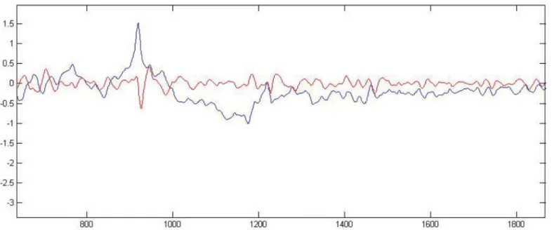
Raw and filtered signals are plotted inFig 1. Filter parameters have remained unchanged and adequate since their first use on a much smaller dataset reported in 2011 [14]. A supervised dataset was built with 9 second pre-countershock signal segments and corresponding
outcomes.
Testing the Basis for Non-Linear Dynamic Methods
Decomposing a short-term/non-stationary, pathological system requires assumptions of lin-earity and periodicity, such as that of the FT, to be relaxed. Limitations of a Fourier based anal-ysis have also been discussed in other studies [15,16]. The Quasi Period Density—Prototype Distance (QPD-PD) method is based on non-linear time-series analysis, which helps in bridg-ing the gap between deterministic chaos theory [16,17] and observed“randomness”of a sys-tem. Methods of non-linear time-series analysis arise from the theory of deterministic dynamical systems [16]. The‘embedding’theorem [18,19] can be used to construct a multidi-mensional phase space from a single variable. Dimensions of the phase space P correspond to multiples of the delayτ.
P¼ ½pn;pn t;. . .;pn ðm 1Þt ð1Þ
The value of each dimension (fromEq 1) at timetcorresponds to the value of the signal at times:t = iΔt,t= (i+τ)Δt,. . .,t ={i+(m-1)τ}Δt, whereiis the sample index. HereΔtserves as
an operator and represents the time between each sample, i.e. (sampling rate)-1of the signal. For afixedm(optimized at 4 dimensions for the given dataset),
1. τhas to be large enough so that the information ati+τis significantly different from the
information ati. Once a properτ(optimized at 8 samples for the given dataset) is chosen it
will give us enough information to construct the phase space.
2. On the other hand, the system may appear not to have any memory ifτis chosen to be too
large.
Based on the optimized parameters, QPD is constructed for each signal. Depending on the actual amount of information (about the system) present in the signal segment (which may partly be a function of the length of the segment),‘loss of memory’is also a characteristic of chaotic systems, where a small change in initial conditions produces a large divergence in tra-jectory in the phase space. It is important to note that the effect of incomplete information about a complex dynamic system (such as the cardiac system in arrest) may produce properties that are similar to that of a chaotic system. In both cases, the system will appear to lose the memory of its initial state and may therefore become unpredictable in time. The Lyapunov exponent [20] quantifies the rate of divergence of two trajectories in the phase space, and would serve to form rationale for non-linear methods used. If the initial separation of two tra-jectories is given byΔS0, they diverge according to the rule
jDSðtÞj ¼elT
jΔS0j ð2Þ
For a discrete time system, whereS0is the starting point of the orbit, andS(t+1) is a function of
S(t), the Lyapunov exponent can be expressed as
l¼lim
n!1 1
n Xn 1
i¼0 lnj
dxiþ1
dxi
j
ð3Þ
chaotic non-linear dynamic characteristics. Additionally, topological mixing is a necessary property of a chaotic system [21], but proving this property is not necessary for our proposed model. The quasi-period plots (Fig 3) can represent deterministic/stochastic, non-dynamical/ dynamical, stable/unstable (chaotic) properties of a system.
Contrastingly, Fourier transform (FT) [22] performs a linear transformation of a function space such that the original signal (function) is decomposed into multiple sinusoids. A tradeoff exists between signal length and frequency resolution. In other words, for a given fixed-dura-tion segment, the Fourier basis is not localized in space/time. Previous studies havenotutilized the above mentioned non-linear dynamic methods for the purpose of predicting defibrillation outcomes. Since QPD’s have a non-linear non-deterministic basis for characterization of ECG’s, the features extracted from them are hypothesized to be strong predictors. This hypoth-esis is proven through statistical testing as well as the relatively strong discriminative perfor-mance of the MDI model as compared to the leading method AMSA.
Feature Extraction and Statistical Analyses
Decomposition and non-linear methods enable us to define and extract characteristics (fea-tures) of a system that may be predictive of the outcomes (success/failure of a shock delivered) and can be used to induct a machine learning model that is predictive of such outcomes. Wave-let Transform (WT) based methods [12] augmented by a dual-tree decomposition algorithm [22] were used to overcome limitations inherent to FT based methods [23] and eliminate shift-variance, which leads to large changes in wavelet coefficients due to small shifts in the signal. Since the signal segments are extracted by windowing, the latter presents a significant problem.
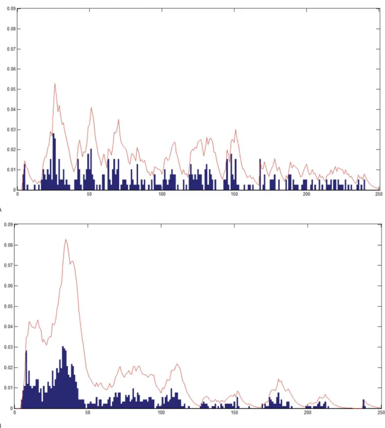
Quasi Period Density—Prototype Distance (QPD-PD): The previously described QPD-PD method [24] was used to characterize chaotic signals from their phase space while allowing for stochasticity/non-determinism. The method's focal point is the Probability Density Function (PDF) of the quasi-period. As illustrated inFig 3, the PDF is calculated by convolving the quasi-period density with the exponential function (Eq 4below). The PDF helps quantify the
Fig 1. Filtering.Blue: Original signal with a sudden jump around sample 900 and then a drift till sample 1200. Red: Filtered signal displaying physiologic morphology around sample 900 and no drift till sample 1200. y-axis::mV, x-axis::samples.
doi:10.1371/journal.pone.0141313.g001
difference in densities between the two classes, 'successful' versus 'unsuccessful'. In the follow-ing convolution,qis the quasi period density andexprepresentse-t/4.
½expqðtÞ ¼
ðþ1
0
expðtÞqðt tÞdt ð4Þ
QPD-PD’s parameter selection and feature calculation are geared for discrimination between classes. Four post-defibrillation signals exhibiting regular sustaining sinus rhythms, with narrow complexes, were used to select the corresponding pre-defibrillation signals as suc-cessful prototypes. Similarly, signals preceding four countershocks that induced minimal change in the ECG or were immediately followed by smooth VF, with no conversion, were selected as unsuccessful prototype signals. The resulting set of (8) pre-countershock signals is termed the Prototype Set (PS). The quantitysep, defined below, is then utilized as the maximi-zation criterion for selection of QPD-PD’s parameters by discriminating successful prototypes from unsuccessful prototypes.
sep¼
X
L
i
KDB
i KDWi
maxð
ffiffiffiffiffiffiffiffiffiffiffiffiffiffiffiffiffiffiffiffiffiffiffiffiffiffiffiffiffiffiffiffiffiffiffiffiffiffiffiffiffiffiffiffiffiffiffiffi
1 CB
X
CBj¼1ðKD j
i KDBiÞ 2
s
;
ffiffiffiffiffiffiffiffiffiffiffiffiffiffiffiffiffiffiffiffiffiffiffiffiffiffiffiffiffiffiffiffiffiffiffiffiffiffiffiffiffiffiffiffiffiffiffiffiffiffiffi
1 CW
X
CWj¼1ðKD j
i KDWi Þ 2
s
Þ ð5Þ
Fig 2. Maximal Lyapunov Exponent of VF.Two boxplots, one for each class, representing distributions of maximal Lyapunov exponent (y-axis) for all signals. x-axis: "0" signifies "unsuccessful" class, while "1" signifies "successful" class.
Fig 3. Quasi-Period Density Function.QPD for (A) a successful shock and (B) an unsuccessful shock. Bars represent the normalized amplitude for each pseudo period: The line curve on top of the histogram represents QPD convolved with the exponential function. If most of the Quasi-Periods are clustered within a small subset of values, as is (B), the convolution helps quantify that fact.
doi:10.1371/journal.pone.0141313.g003
Here,Lis total number of signals from both classes in PS. For a given signali,KDBand
KDWin the numerator are means of distances from PS signals in opposite-class and within-own-class, respectively.CBis the total number of prototype signals in the opposite class while
CWis one less than the number of prototype signals ini’s own class. The distance measureKD
is calculated by comparing the PDFs of quasi-periods [12].KDrepresents the distance of the given signal’s QPD from the QPD of a signal in the prototype set.sepserves to separate the sig-nals in‘successful’PS as far as possible from signals in‘unsuccessful’PS [12]. WhileKDis used for parameter selection,sepcan be used as a general discriminant heuristic that does not neces-sarily need to be defined in terms ofKD.
Sep(Eq 5) is also utilized to calculate the final set of extracted features or explanatory vari-ables. Each scalar value of a feature is representative of one signal segment. We comparesep
with other traditional, well-established parametric and non-parametric heuristic and hypothe-sis tests, namely theFstatistic, analysis of variance (ANOVA) and Mann-Whitney-Wilcoxon (MWW) rank-sum test (Fig 4).
With each unique combination of parameter values for a QPD representation of the signal, one feature-set is constructed. The outcome variable (class) is appended to the vector of fea-tures (explanatory variables) representing a snapshot of the cardiovascular system preceding each countershock. Explanatory variables serve as input to a trained ML model (MDI) which then classifies the corresponding instance to a given class (prediction). To facilitate hypothesis testing, the relationship between outcome and explanatory variables was inverted. Specifically, the class variable can be considered a treatment with two factor levels, successful versus unsuc-cessful, while each explanatory variable would be a measured response.
As the number of features (equivalently, the feature space dimensionality) grows, chances of finding variables that spuriously correlate to outcomes for the given (finite) sample set also grow. This leads to overfitting while training, potentially yielding a seemingly high-performing (on sample set) machine learning model [25]. Additionally, feature and parameter selection on a large number of features become sub-optimal or computationally infeasible [26]. The follow-ing processes and techniques undertaken durfollow-ing the study tackle problems associated with high dimensionality:
• Statistical validation of features through parametric and non-parametric methods, as well as throughmultivariateanalysis of variance.
• Dimensionality reduction
• Parameter selection and feature selection within a nested cross-validation setup
ANOVA assumes a normal distribution for a feature with respect to each class, while KW test is the non-parametric equivalent of ANOVA. KW test can therefore assess features that are non-normally distributed with respect to each factor level (class). Additionally, KW test may serve to be more conservative than ANOVA since our design is not balanced, i.e. class member-ships are imbalanced (218 unsuccessful versus 140 successful). Some loss of information is incurred because continuous feature values are converted to ranks. For the two class case, KW test amounts to a MWW rank-sum test. About 20% of the features extracted showed non-nor-mal skewed histograms for both groups. ANOVA yielded a larger probability of false positives
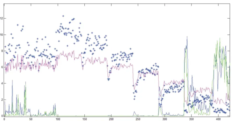
P(fp) where KW test also showed an increasedP(fp) for the corresponding QPD. Each QPD representation corresponds to one unique combination of parameter values. KW test resulted in a higherP(fp) than ANOVA for very few QPD representations (Fig 4), while ANOVA yielded higher P(fp) otherwise.SepandFmeasures agree with each other for all cases, whilesep
shows a greater amount of proportional variance (variance normalized by the mean value) as compared toF. BothFandSepmeasures show a relatively high variance for models 0 through 50. In contrast, for models 300 through 330, the heuristics show smaller variance but also a smaller mean value. Yet, the first 50 representations yield features that lead to large P(fp), even though the values of the heuristics are relatively large. Therefore, increased relative variance within a‘neighborhood’of parameter values may be indicative of spuriously inducted models. This indication is being explored further in a separate study.
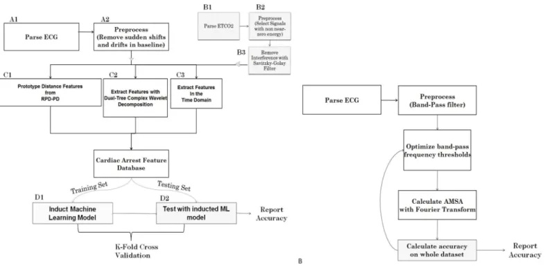
Dual-tree complex wavelet transform and other time-series features were also calculated and incorporated into the feature set [14]. An overview of the system is displayed inFig 5A. QPD-PD and Wavelet-based decomposition constitute data characterization and feature/
Fig 4. Heuristics and Test Statistics.X-axis: Different combinations of parameter values for the QPD-PD method. Y-axis: Scaled Probability of False Positive (for Blue and Green lines) or Values of Measure (for Blue Stars and Pink Line). Blue Stars:Fmeasure, Pink Line:Sepmeasure, Blue Line: ANOVA Probability of False Positive, Green Line: Kruskal-Wallis Probability of False Positive.
doi:10.1371/journal.pone.0141313.g004
information extraction components of the overall MDI system (Fig 5). The final machine learning model that is capable of performing predictions is termed the MDI model here.
Dimensionality Reduction
Projecting the feature space onto a new set of orthogonal axesZis a common technique utilized in many fields ranging from social sciences to microbiology. The technique is used with the hope that the first few dimensions of the new coordinate spaceZwill represent a large majority of the total variance, and that the rest of the dimensions/features can be discarded by making the assumption that the variance represented in them is spurious [25].
The feature set, consisting of distances calculated with QPD-PD, various statistical proper-ties of the wavelet coefficients, and time-series features [12], was first projected onto a new orthogonal set. Each new dimension has a corresponding eigenvalue that quantifies the pro-portion of total variance in the feature set covered by that dimension [25]. Starting from the new feature with the largest eigenvalue and continuing till a cumulative variance close to 99% was reached, the rest (about 40%) of the features from the new set could be discarded [12]. As such, by discarding about 1% of the total variance, a significant reduction in dimensionality was achieved. This makes the subsequent task of feature selection significantly more optimal as well as computationally feasible (data provided inS1 Data).
Prior to dimensionality reduction/orthogonalization, ANOVA served to test each feature with respect to outcomes. Multivariate Analysis of Variance (MANOVA) on the now orthogo-nal feature set provides a holistic answer to the question:‘Is the extracted feature-set signifi-cantly different across classes?’. MANOVA can be seen as an extension of ANOVA for
Fig 5. A. Overview of the MDI system.Components labeled A and B represent pre-processing and filtering. C represent non-linear modeling, decomposition, and feature extraction. D represent machine learning model induction and testing. Additional statistical analyses such as KW test and MANOVA were performed with the feature database created by C.B. AMSA feature/method.Flowchart represents the sequence of steps involved in the AMSA method, with the two major methodological components being the filtering (low-pass and band-pass) and the Fourier Transform.
multiple dependent variables that are preferably uncorrelated, since collinearity can lead to unstable estimate of discriminant function coefficients and an increasing number of (corre-lated) responses results in loss of degrees of freedom, thereby limiting benefit. Additionally, reduced dimensionality results in increased robustness to heterogenous variance-covariance matrix. In order to conduct MANOVA, dimensions from the uncorrelated feature set were treated as responses and the class was treated as a factor. Notably, MANOVA for two factor levels reduces to a multivariate T-squared test.
Comparing ML Paradigms and Algorithms
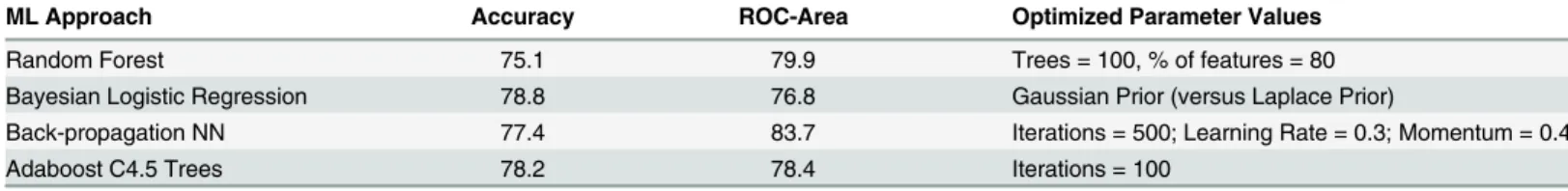
Inductive ML algorithms can create a mathematically expressible function, as demonstrated in numerous decision rules in medicine derived from logistic regression [26]. For example, a number of risk scores, such as TIMI, have been developed for predicting the risk for cardiovas-cular complications [27]. The‘No Free Lunch’theorem [28] establishes that no specific algo-rithm can be guaranteed to provide the highest performing model for a given finite dataset. Multiple ML methods, including back-propagating neural networks,19Random Forest Tree Induction [29], and traditional Bayesian logistic regression [30] were utilized to induct models with the supervised feature sets. We selected algorithms that are well-known in the field of machine learning, have been researched thoroughly for several years. All performance metrics for the inducted MDI models are presented inTable 1.
Receiver Operating Characteristic (ROC) analysis was used to evaluate reliability of all mod-els by calculating the area under the curve (AUC). Accuracy was calculated as the average per-centage, over all cross-validation runs, of instances correctly classified. Allaccuracy,sensitivity
andspecificityvalues are reported for the best decision threshold found for the given test and/ or algorithm. These statistical measures are reported at both 80% and 90% sensitivity levels. Conservative nested ten-fold cross-validation, in which parameters are selected inside the training sets to avoid overfitting, was used for all tests so as to obtain an unbiased estimate of accuracy, sensitivity and specificity. In this validation process, data is randomly divided into ten partitions (folds). During each step of validation process (i.e. each outside loop), a combi-nation of nine partitions is used for training the MDI model while the last partition is used for testing the trained model. This process is repeated ten times, each time using a previously unused fold for testing.
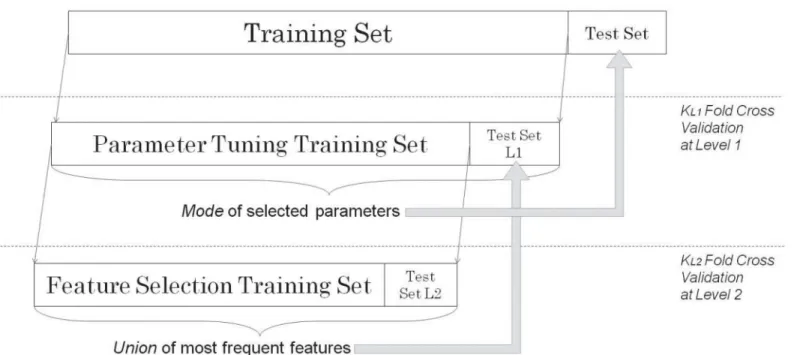
In nested architecture (Fig 6), for each outside loop, a subset of data inside the combined nine training sets is used for selection of features for the model. As such, the selected features vary for each outermost test fold, while the global set of features (as well as feature extraction and selection algorithms) stay constant. This feature selection process significantly reduces the chances of overfitting (positive bias on reported accuracy) with respect to parameter selection process [11]. In contrast, the AMSA (Fig 5B) method does not employ cross-validation or nested cross validation in order to select parameters (such as frequency sub-band, filtering threshold) or to estimate performance metrics.
Table 1. Results of each compared Machine Learning Approach.
ML Approach Accuracy ROC-Area Optimized Parameter Values
Random Forest 75.1 79.9 Trees = 100, % of features = 80
Bayesian Logistic Regression 78.8 76.8 Gaussian Prior (versus Laplace Prior)
Back-propagation NN 77.4 83.7 Iterations = 500; Learning Rate = 0.3; Momentum = 0.4
Adaboost C4.5 Trees 78.2 78.4 Iterations = 100
doi:10.1371/journal.pone.0141313.t001
Results and Discussion
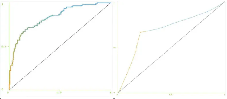
Classification using MDI with additive logistic regression [31] as a classifier, with up to 20 fea-tures, yielded an ROC AUC of 83.2% for the model built with ECG data only (Fig 7A). Multiple comparisons of MDI and previously reported AMSA method [23] were performed. AMSA yielded an ROC AUC of 69.2% (Fig 7B).
Specificity can be calculated at desired levels of sensitivity by adjusting the decision thresh-old of a classifier. If the classifier’s output is continuous, this threshthresh-old can be set anywhere within the range of the output. For logistic regression, continuous values between 0 and 1 rep-resent the probability of a successful shock according to the model. At 80% sensitivity (thresh-old of .41), MDI provided an accuracy of 74% and specificity of 70.2%. At the same level of sensitivity (80%), AMSA provided an accuracy of 53.6% and specificity of 36.7%. While increasing that sensitivity to 90% (threshold of .22) yielded an accuracy of 68.4% and specificity of 54.6% with MDI, performance of AMSA dropped dramatically to 43.3% and 13.3% respec-tively (Table 2).
Integrating PetCO2 features into MDI boosted ROC AUC to 93.8% for a total of 48 shocks with usable CO2 signal segments. At 90% sensitivity, the large ROC AUC allowed for 83.3% accuracy and 78.6% specificity.
MANOVA was carried out on the resulting orthogonal (uncorrelated) feature set, yielding (p<0.05), and thus rejecting the null hypothesis that the class (outcome) is not associated with
different pre-countershock cardiac states as represented by the set of features.
Predicting the success of defibrillation would minimize interruptions in CPR and unneces-sary shocks, both of which can reduce chances of ROSC and ultimate survival to discharge. Physiologic changes during CPR take place over short intervals as the compressions and
Fig 6. Framework for Wrapper Based Hyper-Parameter Selection.Twice-nested cross-validation setup. Parameter tuning is performed at Level 1 (L1), where an optimal feature subset has already been selected by cross-validation at Level 2 (L2). k = kL1= kL2= 10 folds; same for all levels.
pharmacotherapy attempt to improve myocardial perfusion. In the study presented, the MDI model was able to discriminate with high accuracy those defibrillations that effectively con-verted VF to a perfusing rhythm and those that did not. Predictions are computed in real-time (<.08 second delay per prediction) and are based on information gathered from signal seg-ments 9 seconds in duration.
A few predictors of successful resuscitation exist. These include physiologic parameters such as coronary perfusion pressure (CPP) [31], central venous oxygen saturation (Scvo2) [32], PetCO2[33,34], and QVM of the ECG waveform [35,36]. While directly correlated to cardiac output and highly sensitive for ROSC, CPP and Scvo2are mostly impractical to measure during cardiac arrest outside of the intensive care unit (ICU) setting. Waveform capnography to mea-sure PetCO2is practical in most settings, including the pre-hospital environment, and is highly correlated with CPP [37], cerebral perfusion pressure [38], and ROSC [39,40]. However, its ability to predict defibrillation success has not been established.
Without an ideal monitoring technique to predict the success of defibrillation that is practi-cal in all cardiac arrest settings, QVM has emerged as a technology that can be integrated into existing defibrillator units. The most prominent, AMSA, relies upon a single feature of VF derived from the Fourier Transform to predict defibrillation success. In certain animal [41,42] and human [23,43] investigations, AMSA has been shown to predict defibrillation success with
Fig 7. Receiver Operating Characteristic curves.For (A) MDI model built using all 358 shocks, (B) AMSA method. X-axis = 1-Specificity, Y-axis = Sensitivity. Threshold ranges from 0 to 1 as the color transitions from orange to blue from one end to the other.
doi:10.1371/journal.pone.0141313.g007
Table 2. Performance of the MDI model in comparison with AMSA.
Accuracy Proposed Model AMSA Feature
Overall 78.8% 73.9%
80% Sensitivity 74% 53.6%
90% Sensitivity 68.4% 43.3%
ROC-Area 83.2% 69.2%
doi:10.1371/journal.pone.0141313.t002
greater than 90% sensitivity and specificity. However, these studies did not employ cross-vali-dation in their analyses, which yields an unbiased and significantly more conservative estimate of performance for unseen data while utilizing the entire dataset available. Although statisti-cally significant, generalization performance of AMSA as a discriminator has been found to be much lower in recent studies [11]. The feature and parameter selection framework for MDI allows us to judge the success of current research efforts and to provide the right foundation for potential translational research.
In the field of artificial intelligence, the technique of ML is capable of utilizing numerous features extracted from a signal(s) to identify significant patterns, which match a classification of interest. In this case the classification of successful versus unsuccessful defibrillation is used. Each one of the features can contain information that is complementary to the information present in other features. All such discriminative information is integrated into a predictive model using ML. As such, the models may provide higher power of discrimination, measured through ROC curves and accuracy [12,14]. These techniques can be particularly useful in pro-cesses deemed to be nonlinear in nature.
Methods of feature extraction represent another link in the computational chain of steps involved. The dual-tree complex wavelet transform used in this study provides both time and frequency localization for non-stationary signals. In contrast, FT decomposes a signal into sinusoids that are globally averaged. Therefore, information that is transiently present over a limited period (i.e. time resolution) is lost. Furthermore, the field of non-linear dynamics pro-vides appropriate methods for characterizing chaotic data. QPD-PD method is able to capture the non-linear dynamical nature of VF signal in order to extract features. In contrast, FT is severely limited in its capabilities to properly decompose non-stationary biomedical signals due to its linear and deterministic assumptions, in order to extract the features.
A QVM approach that relies solely upon one ECG feature to predict defibrillation success may suffer from random effects [44]. In contrast to the single feature AMSA technique, the ML approach is able to integrate multiple features in order to construct a more complete/robust model capable of predicting shock success for cardiac arrest victims with greater accuracy. The approach described allows for integration of information from multiple signals, not just multi-ple features from one signal.
Introduction of other independent but temporally related signals, in this case PetCO2, may also help to significantly offset the random effects inherent to ECG features as demonstrated by the increase in sensitivity, specificity, and ROC AUC in the combined signal model. It is not surprising that PetCO2 is helpful in this regard given its relationship to cardiac output and CPP during CPR [45]. Thus, this and other indicators of perfusion may further enhance the performance of an ML based approach to real-time predictive clinical decision-support.
Whenever cross-validation is employed with feature selection or parameter tuning, a twice-nested implementation is requisite for obtaining results that are unbiased by information in the test set. This follows the assumption that field application will produce previously unseen data, providing a true test for the model. Additionally, there is usually a tradeoff between complexity of the predictive model and its generalization performance. As complexity is partly a function of the number of features, type of ML learning algorithm, and its parameters, nested cross-vali-dation also provides a way to optimize this tradeoff.
post-countershock period (such as 90 seconds for AMSA) confounds the cause of an outcome for decision support model development purposes. On the other hand, not being able to resume CPR for observational sake would be even more problematic. Defibrillation success is also influenced by post-shock pauses, thereby supporting the use of shorter, clinically relevant, definition of ROSC [47,48].
The authors recognize some important limitations to our findings presented here. This anal-ysis was conducted retrospectively upon 358 defibrillation attempts of 153 victims of VF car-diac arrest and our measured outcome, initial ROSC, does not include survival to hospital discharge. Pre-shock pauses and“no-flow”time before defibrillation were not controlled for and have been shown to influence defibrillation success [49]. Additional factors such as certain drugs in the bloodstream, ischemic cardiomyopathy may confound defibrillation success. Cases presenting electromechanical dissociation would not benefit from the proposed model. PetCO2, while shown to dramatically improve the sensitivity and specificity of the model, was not available for all ECG tracings.
Conclusion
For a given desired sensitivity, MDI provides a significantly higher accuracy and specificity than AMSA in yielding far fewer futile defibrillations (i.e. false positives). Various assumptions underlying feature extraction survive validation through multivariate statistical and non-linear methods. Addition of PetCO2improves the ROC and sensitivity of MDI prediction model. A combined use of appropriate nonlinear modeling techniques, multiple physiologic signals, and machine learning techniques that integrate information from multiple features should facilitate more robust performance when creating predictive physiologic indices for use during cardiac arrest resuscitation.
Supporting Information
S1 Data. Sample dataset with Shock Outcome coded as the last column labeled‘SO’, and principal component predictive attributes/features represented by the rest of the columns. (CSV)
Author Contributions
Conceived and designed the experiments: SS KN. Performed the experiments: SS. Analyzed the data: SS. Wrote the paper: SS MCK KRW KN.
References
1. Go AS, Mozaffarian D, Roger VL. Heart disease and stroke statistics—2013 update: a report from the
American Heart Association. Circulation, 2013; e6–e245.
2. Nichol G, Thomas E, Callaway CW. Regional variation in out-of-hospital cardiac arrest incidence and outcome. J Am Med Assoc, 2008; 300:1423–31.
3. Beck CS, Pritchard WH, Feil HS. Ventricular fibrillation of long duration abolished by electric shock. J Am Med Assoc, 1947; 135:985. PMID:20272528
4. Stiell IG, Nichol G, Leroux BG. Early versus later rhythm analysis in patients with out-of-hospital cardiac arrest. N Engl J Med, 2011; 365:787–97. doi:10.1056/NEJMoa1010076PMID:21879896
5. Sato Y, Weil MH, Sun S. Adverse effects of interrupting precordial compression during cardiopulmo-nary resuscitation. Crit Care Med, 1997; 25:733–6. PMID:9187589
6. Steen S, Liao Q, Pierre L, Paskevicius A, Sjoberg T. The critical importance of minimal delay between chest compressions and subsequent defibrillation: a haemodynamic explanation. Resuscitation, 2003; 58:249–58. PMID:12969599
7. Yu T, Weil MH, Tang W. Adverse outcomes of interrupted precordial compression during automated defibrillation. Circulation, 2002; 106:368–72. PMID:12119255
8. Tang W, Weil MH, Sun S. The effects of biphasic waveform design on post-resuscitation myocardial function. J Am Coll Cardiol, 2004; 43:1228–35. PMID:15063435
9. Xie J, Weil MH, Sun S. High-energy defibrillation increases the severity of postresuscitation myocardial dysfunction. Circulation, 1997; 96:683–8. PMID:9244243
10. Firoozabadi R, Nakagawa M, Helfenbein ED, Babaeizadeh S. Predicting defibrillation success in sud-den cardiac arrest patients. J Electrocardiol, 2013; 46:473–9. doi:10.1016/j.jelectrocard.2013.06.007
PMID:23871657
11. Nakagawa Y, Sato Y, Kojima T. Amplitude spectral area: predicting the success of electric shock deliv-ered by defibrillators with different waveforms. Tokai J Exp Clin Med, 2013; 38:71–6. PMID:23868738 12. Shandilya S, Ward K, Kurz M, Najarian K. Non-linear dynamical signal characterization for prediction of defibrillation success through machine learning. BMC Medical Informatics and Decision Making, 2012; 12:116. doi:10.1186/1472-6947-12-116PMID:23066818
13. Hall Mark, Frank Eibe, Holmes Geoffrey, Pfahringer Bernhard, Reutemann Peter, Witten Ian H.; The WEKA Data Mining Software: An Update. SIGKDD Explorations, 2009, 11; Issue 1.
14. Shandilya S, Kurz M, Ward KW, Najarian K. Predicting defibrillation success with a multiple-domain model using machine learning. IEEE/ICME International Conference on Complex Medical Engineering (CME). Harbin, China 2011:9–14.
15. Watson JN, Uchaipichat N, Addison PS, Clegg GR, Robertson CE, Eftestol T. et al. Improved prediction of defibrillation success for out-of-hospital VF cardiac arrest using wavelet transform methods. Resusci-tation, 2004; 63: 269–275. PMID:15582761
16. Kantz H, Schreiber T. Nonlinear Time Series Analysis. new edition Cambridge, New York: Cambridge University Press; 1999.
17. Werndl Charlotte. "What are the New Implications of Chaos for Unpredictability?". The British Journal for the Philosophy of Science, 2009; 60 (1): 195–220.
18. Takens F. Detecting Strange Attractors in Turbulence. Lecture Notes in Mathematics. 898: 366–1981. 19. Sauer T, Yorke J A, Casdagli M. Embedology. J. Stat. Phys, 1991. 65: 579–616.
20. Brown R, Bryant P, Abarbanel H. "Computing the Lyapunov spectrum of a dynamical system from an observed time series". Physical Review A, 1991; 43(6): 2787. PMID:9905344
21. Vellekoop M, Berglund R. On Intervals, Transitivity = Chaos. The American Mathematical Monthly, 1994; 101(4): 353–5.
22. Ristagno G, Gullo A, Berlot G, Lucangelo U, Geheb E, Bisera J. Prediction of successful defibrillation in human victims of out-of-hospital cardiac arrest: a retrospective electrocardiographic analysis. Anaesth Intensive Care, 2008; 36: 46–50. PMID:18326131
23. Kingsbury NG. The dual-tree complex wavelet transform: A new efficient tool for image restoration and enhancement. Rhodes: Proc European Signal Processing Conf, 1998; 319–322.
24. Shandilya S, Qi X, Najarian K, Ward K, Hargraves R. Finding an Optimal Model for Prediction of Shock Outcomes through Machine Learning. The Eighth International Multi-Conference on Computing in the Global Information Technology, Nice, France; 2013: 214–8.
25. Duda RO, Hart PE, Stork DG. Pattern Classification. Wiley; 2001.
26. Quinlan R. Programs for Machine Learning. Morgan Kaufmann Publishers; 1993.
27. Antman EM, Cohen M, Bernink PJ, et al. The TIMI risk score for unstable angina/non-ST elevation MI: A method for prognostication and therapeutic decision making. J Am Med Assoc 2000; 284:835–42. 28. Wolpert D.H., Macready WG, "No Free Lunch Theorems for Optimization", IEEE Transactions on
Evo-lutionary Computation, 1997; 1: 67.
29. Brieman L. Random Forests. Machine Learning, 2001; 45: 5–32.
30. Genkin A, Lewis DD, Madigan D. Large-scale bayesian logistic regression for text categorization. Tech-nometrics, 2007; 49: 291–304.
31. Friedman J, Hastie T, Tibshirani R. Additive logistic regression: a statistical view of boosting. Annals of Statistics, 2000; 28: 337–407.
32. Paradis NA, Martin GB, Rivers EP, et al. Coronary perfusion pressure and the return of spontaneous circulation in human cardiopulmonary resuscitation. J Am Med Assoc, 1990; 263: 1106–13.
34. Levine RL, Wayne MA, Miller CC. End-tidal carbon dioxide and outcome of out-of-hospital cardiac arrest. N Engl J Med, 1997; 337: 301–6. PMID:9233867
35. Wayne MA, Levine RL, Miller CC. Use of end-tidal carbon dioxide to predict outcome in prehospital car-diac arrest. Ann Emerg Med, 1995; 25:762–7. PMID:7755197
36. He M, Chen B, Gong Y, Wang K, Li Y. Prediction of Defibrillation Outcome by Ventricular Fibrillation Waveform Analysis. Clinical & Experimental Cardiology, 2013:1–8.
37. Reynolds JC, Salcido DD, Menegazzi JJ. Correlation between coronary perfusion pressure and quanti-tative ECG waveform measures during resuscitation of prolonged ventricular fibrillation. Resuscitation, 2012; 83: 1497–502. doi:10.1016/j.resuscitation.2012.04.013PMID:22562057
38. Sanders AB, Atlas M, Ewy GA, Kern KB, Bragg S. Expired PCO2 as an index of coronary perfusion pressure. Am J Emerg Med, 1985; 3: 147–9. PMID:3918548
39. Lewis LM, Stothert J, Standeven J, Chandel B, Kurtz M, Fortney J. Correlation of end-tidal CO2 to cere-bral perfusion during CPR. Ann Emerg Med, 1992; 21: 1131–4. PMID:1514728
40. Callaham M, Barton C. Prediction of outcome of cardiopulmonary resuscitation from end-tidal carbon dioxide concentration. Crit Care Med, 1990; 18: 358–62. PMID:2108000
41. Sanders AB, Kern KB, Otto CW, Milander MM, Ewy GA. End-tidal carbon dioxide monitoring during car-diopulmonary resuscitation. A prognostic indicator for survival. J Am Med Assoc, 1989; 262: 1347–51. 42. Marn-Pernat A, Weil MH, Tang W, Pernat A, Bisera J. Optimizing timing of ventricular defibrillation. Crit
Care Med, 2001; 29: 2360–5. PMID:11801840
43. Povoas HP, Weil MH, Tang W, Bisera J, Klouche K, Barbatsis A. Predicting the success of defibrillation by electrocardiographic analysis. Resuscitation, 2002; 53: 77–82. PMID:11947983
44. Young C, Bisera J, Gehman S, Snyder D, Tang W, Weil MH. Amplitude spectrum area: measuring the probability of successful defibrillation as applied to human data. Crit Care Med, 2004; 32: S356–8.
PMID:15508659
45. Gundersen K, Kvaloy JT, Kramer-Johansen J, Eftestol T. Identifying approaches to improve the accu-racy of shock outcome prediction for out-of-hospital cardiac arrest. Resuscitation, 2008; 76: 279–84.
PMID:17767991
46. Wang H. Intra-arrest selective brain cooling improves success of resuscitation in a porcinemodel of pro-longed cardiac arrest. Resuscitation, 2010; 81: 617–621.
47. Sayre MR, Koster RW, Botha M. Part 5: Adult basic life support: 2010 International Consensus on Car-diopulmonary Resuscitation and Emergency Cardiovascular Care Science With Treatment Recom-mendations. Circulation, 2010; 122: S298–324.
48. Berg RA, Hemphill R, Abella BS. Part 5: adult basic life support: 2010 American Heart Association Guidelines for Cardiopulmonary Resuscitation and Emergency Cardiovascular Care. Circulation, 2010; 122: S685–705. doi:10.1161/CIRCULATIONAHA.110.970939PMID:20956221
49. Cheskes S, Schmicker RH, Christenson J. Perishock pause: an independent predictor of survival from out-of-hospital shockable cardiac arrest. Circulation, 2011; 124: 58–66.