A Work Project, presented as part of the requirements for the Award of a Master Degree in
Economics from NOVA – School of Business and Economics.
DEMOCRACY AS A
CURVE
Henrique Marques Ucha Meireles Alpalhão
#827
A project carried out on the Master in Economics Program, under the supervision of:
Professor Paulo Rodrigues
Democracy as a Curve
Abstract
This paper attempts to model the widely studied relationship between a country's economic
growth and its level of democracy, with an emphasis on possible non-linearities. We adopt the
concept of “political capital” as a measure of democracy, which is extremely uncommon in the
literature and brings considerable advantages both in terms of dynamic considerations and
plausibility. While the literature is not consensual on this matter, we obtain significant and robust
results that indicate that the impact of democratization on economic growth varies according to
the stage of democratic development each country is in.
Keywords
Democracy, Economic Growth, Political Capital, Political Economy
Acknowledgements
The author is deeply grateful to Professor Paulo Rodrigues (Nova SBE) for his guidance and
availability. This study has additionally benefitted from important suggestions from Professor
Pedro Magalhães (Institute of Social Sciences (ICS) – University of Lisbon). The author further
dearly acknowledges the input and concern of his fellow Nova SBE teaching assistants at office
1, as well as all remaining comments and suggestions by close and loved ones. A special thank
you goes to the author’s father, who is the reason why the author will most likely always be cited
I. Introduction
The concept of democracy is present across various dimensions of our civilization. The
institution and maintenance of democracy is one of the most defining plights of human society in
the last centuries, and a democratic way of rule is widely culturally regarded as a value in itself.
This is arguably mostly based on the value of equity, which is a main objective of democracy. In
economic terms, we could argue that it is an expression of the efficiency-equity trade-off – one
may suggest that centralization might bring about efficiency gains1, but it is most certainly equity
reducing.
Looking at the literature, however, one finds no clear consensus on whether democracy increases
or decreases economic performance. Assessing it objectively is made difficult for two reasons:
firstly, evaluating how democratic a country is will always be at least somewhat subjective;
secondly, one would expect the impact of democratization on economic performance to depend
on a country’s level of democratization itself, since a dictatorship’s first steps into democracy
and the improvement of an already democratic way of rule are unquestionably different
processes. This dynamic component has, as far as we are aware, been largely ignored in the
existing literature.
This paper will attempt to shed some light on this matter – to establish the economic
performance of a country as a function of its level of democratization, modeling the relationship
as a curve and allowing for inflexion points.
The use of a broad database encompassing more than 60 countries over several years
(approximately 2400 observations) means that we are not studying specific countries, but
modern society and its democracies – empowered by an extensive dataset, we attempt to better
understand how economy and democracy relate.
1
This paper is organized as follows: section II provides an overview of the existing literature on
this matter. Section III theoretically discusses the novelty of our approach. Section IV describes
the data we use, while section V presents and explains the model. Section VI details obtained
results. Section VII contains robustness checks to our results. Finally, section VIII concludes.
II. Literature review
The literature on the impact of democracy on economic growth or income, henceforth referred to
as economic performance, is extensive – the conclusions, however, are not consensual. The
existing research is divided between those who find that democratization decreases economic
performance (Barro, 1996; Tavares and Wacziarg, 2001), those that find that it increases
economic performance (Gerring et al., 2005; Acemoglu et al., 2014; Knutsen, 2015; Madsen et
al., 2015) and those that find that it has had no significant impact (Helliwell, 1994).
The avenues through which democratization could impact economic performance have,
similarly, been the topic of a large branch of literature. Increased human capital accumulation
(Tavares and Wacziarg, 2001; Corujo and Simões, 2012; Acemoglu et al., 2014), lower income
inequality (Tavares and Wacziarg, 2001), better protection of property rights (Leblang, 1996;
Clague et al., 2003; Knutsen, 2011), the fostering of technological growth (Coccia, 2010), the
elimination of the risk of “predatory rulers” (Krieckhaus, 2006; Knutsen, 2012), openness to
non-elites and the institutional flexibility that democracy implies (Acemoglu, 2008; Davis, 2010)
and finally the encouragement of investment, economic reforms, better public good provision
and reduced social unrest (Acemoglu et al., 2014) are the main reasons found for a positive
relationship. On the other hand, reduced physical capital accumulation and higher government
consumption in relation to GDP (Tavares and Wacziarg, 2001), increased vulnerability to
interest groups and lobbies (Olson, 1982; Wade, 1990; Doucouliagos and Ulubaşoğlu, 2006),
Krieckhaus, 2006) and the wealth redistribution from rich to poor that democracies tend to enact
(Barro, 1996) are some of the factors that suggest that democratization may reduce growth.
Finally, some studies with a dichotomous emphasis (autocracy vs. democracy) offer interesting,
more specific insight on the matter at hand. De Luca et al. (2015), building on Olson (1993),
show how an own-wealth maximizing capital-rich dictator may generate higher growth than
what would occur in a democracy. On this same issue, Doucouliagos and Ulubaşoğlu (2006)
argue that an autocracy could be superior to a democracy in terms of growth due to myopic
voting behavior – in a democracy, voters may prefer higher consumption today at the expense of
investment, which would bring about future welfare gains. Madsen et al. (2015), using a very
broad database (from 1500 to 2000), reach the conclusion that democracy did positively impact
income growth in their sample. Acemoglu et al. (2014) also make a very compelling argument
for a positive relationship (“Democracy does cause growth”), which is in line with the recent
academic tendency.
Since the construction of a variable that measures the level of democratization of each country
for a long time period seems a quite technical and daunting enterprise, papers such as this one
must either rely on existing variables for this purpose or face the challenge of creating a new
one. The literature offers several options – for this investigation, we have considered the Polity
IV project (Marshal et al., 2016), Tatu Vanhanen’s Polyarchy Index (Vanhanen, 2002), The
Democracy Ranking Association’s Democracy Ranking (Campbell, 2008), the Unified
Democracy Scores (UDS) (Pemstein et al., 2010) and the Latent Democracy Variable (LDV)
(Foldvari, 2014). The first two are the most widely used and accepted ones. The Polyarchy Index
is the simplest, factoring political competition and participation equally as a measure of
democracy. Polity IV’s polity2 variable offers, in our view, several advantages relatively to
Vanhanen’s data: it takes more factors into account (such as constraints on the executive, for
(negative values). Additionally, according to Pemstein et al. (2010), the Polity IV project offers
one of the top three higher reliabilities among existing democracy scales, while Vanhanen’s
measure often differs significantly from other scores. Further reading into Pemstein et al.,
however, allows us to identify some caveats with Polity IV’s data – notably, that the mid-section
of the ranking may be significantly overlapping (small differences in this range seem, as such,
potentially arbitrary). Treier and Jackman (2008) also discuss the issues with this index at length,
stressing the information loss that occurs in the aggregation of each partial score (so that quite
different regimes may be evaluated in the same way if their scores add up the same), the
arbitrary aggregation method and the presence of a measurement error within the variable (which
is usually overlooked when the index is applied in research). While we recognize its strengths,
we take these criticisms into account and therefore approach this variable with care.
The Democracy Ranking is the most particular measure we have found – it uses not only
political, but also economic and development indicators to build a “complete” measure of
democracy – democracy as societal evolution. While we regard the concept as quite interesting
and have considered using the ranking for our analysis, ultimately its small scope (little more
than 10 years), lack of presence in the literature and potential for endogeneity have made us opt
for different measures.
Treier and Jackman (2008) stress that democracy is a latent variable – it is not directly observed,
but rather has to be constructed from observed or theorized measures. A possible way to curb
this issue is to use a variable such as the LDV or UDS – measures extracted from several
existing indexes of democratization with the goal of minimizing measurement errors. Since LDV
is extracted only from the Polity IV and Polyarchy Index scales and UDS, conversely, takes 8
more existing measures into account (and both cover our 1960-2010 timeframe equally), the
Unified Democracy Scores seem a more attractive option. Pemstein et al. (2010), in order to
country-year, [our variable] is at least as reliable as the most reliable component measure”. Like the
polity2 variable, the UDS are also presented in a scale that encompasses positive and negative
values.
From our survey of the available democracy measures, we find two variables that seem adequate
for our estimation: Polity IV project’s polity2 due to its wide acceptance in the literature2 and the
UDS by Pemstein et al. due to its tackling of all major issues we find with the former index.
As has been mentioned before, our aim is to investigate the existence of a non-linear relationship
between economic growth and democratization. This has been studied in a small fraction of the
literature – specifically, Barro (1996) finds significance for an inverted-U-shaped relationship
(there is a level of democracy that maximizes growth), using a database of 100 countries from
1960 to 1990. We regard these conclusions as the basis of our study and intend to augment it via
a longer timeframe, the possibility of more than one inflexion point and the use of different
political data (notably, the use of a political capital variable). Alfano and Baraldi (2016) have
found the same relationship using data for political competition on 83 countries from 1979 to
2011. While we expect to back their results, we believe political competition to be an insufficient
measure to effectively characterize a country’s political system.
III. Theoretical discussion
As we have attempted to show with section II, the literature on the democracy/growth
relationship is extensive. We find, however, that estimations almost invariably take the form of a
regression or series of regressions using growth as the dependent variable and a lagged variable
that measures how democratic a country was in a specific year as the main independent variable.
This framework, in our opinion, presents two major caveats:
2 Gerring et al. (2005), Coccia (2010), Corujo and Simões (2012), Murtin and Wacziarg (2014), Madsen et al.
a) The use of a political measure for a specific year only (a “democracy flow”);
b) The assumption that the relationship should be linear.
Regarding a), the use of a lagged democracy flow ignores all previous democratic history, since
a just democratized country’s positive political index score and the score of a long-running
democracy are viewed by the model as the same. This seems overly simplistic – we will, as such,
attempt to use the more realistic formulation of a political stock: the accumulation of democratic
governance throughout the years. In our robustness section, we turn to the democracy flow
method to allow for comparisons.
Caveat b) is, in our opinion, equally as relevant – it gains, however, increased weight when we
model democracy as a stock rather than a flow. When we assume linearity, we are effectively
saying that a change in the level of democratization of a country will have the same impact on
economic growth, regardless of how democratic society was to start with. It is not difficult to
argue against this view – the many, potentially opposing effects detailed in section II could very
plausibly have different weights depending on the level of democratic evolution. Take, for
instance, the increased openness to non-elites that should increase growth when a country
becomes more democratic – a quite democratic country should have already taken measures with
such an objective in the past. As such, increased growth via this avenue should, from a certain
point onwards, cease to become substantial. Arguments such as this make it seem quite plausible
that there is a certain stock that maximizes growth – countries beyond that could, for various
reasons detailed in section II, sacrifice growth for other goals or simply stifle it.
To address a), we follow Gerring et al. (2005) and their political stock concept – the construction
of the stock variable will be detailed in section V. In regards to b), we adopt a model that
includes political stock as its main independent variable as well as political stock to the power of
2 to 6, so as to attempt to identify any existing non-linearities. The number of inflexion points is
significance for a quadratic formulation, but we find it plausible that at least a second inflexion
point occurs, especially since our scale encompasses both the level of autocracy (negative
values) and democracy (positive values), and these may relate to growth differently.
IV. Data
The polity23 variable from the Polity IV project endows us, before treatment, with 215 years
(1800-2015) of data on more than 150 countries – this makes it a quite powerful instrument. The
Unified Democracy Scores4, on the other hand, cover the 1946-2012 timeframe for more than
110 countries.
For economic and demographic data, we have used both World Bank’s and Clio-Infra project’s
online databases5. These have effectively reduced our database to the years of 1960-2010, and as
such nullified the longer timeframe advantage of polity2.
After treatment (in order to eliminate missing values of economic growth and political indexes),
we work with a yearly database of 51 years and 66 countries, amounting to 3366 observations.
Our choice of controls follows a simple method: we survey the literature for controls in growth
regressions and choose those that fit our purpose and do not display a non-stationary behavior.
They are the following:
• Electric power consumption in KWh per capita as a proxy for GDP per capita6;
• Natural logarithm of population growth (Mauro, 1995; Alfano and Baraldi, 2016);
3 For details on the construction of this variable, refer to Marshal et al. (2016). Data originate from
http://www.systemicpeace.org/inscrdata.html.
4
For details on the construction of this variable, refer to Pemstein et al. (2010). Data originate from http://www.unified-democracy-scores.org/uds.html. Missing UDS values for Jamaica have been obtained from the Clio-Infra project’s database (https://www.clio-infra.eu/).
5
Specifically, electric power consumption, GDP, population and trade data have been obtained from the World Bank (http://data.worldbank.org/indicator) and inflation from Clio-Infra (https://www.clio-infra.eu/).
6
• International trade (imports+exports) as a percentage of GDP (Gerring et al., 2005;
Acemoglu et al., 2014);
• Inflation rate (Gerring et al., 2005).
With these, we believe we strike the right balance between covering the main dimensions that
impact growth and parsimony. We purposely leave several common controls, such as human
capital, unaccounted for – we want all indirect avenues through which democracy impacts
growth to be included in our democracy variable’s impact7.
Electric power consumption is intended as a proxy for GDP per capita. It represents the
convergence theory – poorer countries tend to grow faster than rich ones, so that eventually
income levels should converge. Population growth, which could also be measured with fertility
rates, represents the idea that an economy will grow less if more resources are affected to
childbearing and extra capital is required to equip the new generations (whilst, with lower
population growth, capital per worker would grow more with investment). This is in line with
Barro (1996). International trade, on the other hand, is meant to measure trade openness, which
seems an important factor for economic growth and is not necessarily a characteristic of
democratic or autocratic societies. Tavares and Wacziarg (2001) discuss how protectionism may
occur both in democracies and autocracies, as agents who benefit from protection can generally
mobilize more easily than the remaining population regardless of the regime. Finally, Barro
(1995) has established a negative relationship between inflation and growth – we control, as
such, for the change in the general price level of the economy. This is again based in the notion
that inflation may affect countries regardless of their democratic development, especially when it
is due to international events, such as, for example, an oil shock.
The differing distributions of missing values along our control variables have brought upon us
the choice of either using an unbalanced panel or severely limiting the number of observations in
7
our study. We have opted for the former, in line with a significant part of our literature (such as
Acemoglu et al., 2014 or Madsen et al., 2015). The elimination of missing values brings our
database to its final version, with 2406 observations.
Below, we present a series of tables. Table 1 displays descriptive statistics for our used variables.
Table 2 reports the unit root test results, while table 3 displays the variance-covariance matrix
between our variables. Appendix A1 further presents a list of used countries, as well as their
respective polity2 and UDS scores in 1960 and 2010 – it shows that our sample is not only
adequately diverse geographically, but also in terms of democratic starting and finishing
“positions”. It further gives us some insight on the similarities and differences between polity2
and UDS8.
Table 1. Descriptive statistics
Variable Observations Mean Std. Dev. Min Max
GDP growth 3300 .020616 .0429822 -0.3086214 0.5704207
Electric consumption 2739 3352.337 4169.772 14.68682 25590.69
Population growth 3150 12.26891 1.63813 2.079442 16.94183
Trade openness 3149 55.51591 29.7706 4.920835 220.4073
Inflation 3162 38.27432 514.3589 -20.07576 23773.13
polity2 3366 3.116756 7.470499 -10 10
UDS 3366 0.3376526 1.043991 -2.112144 2.262576
Table 2. Results for the Im-Pesaran-Shin unit-root tests9
Variable p-value (demeaned)
GDP growth 0.0000
Electric consumption 0.0899
Population growth 0.0000
Trade openness 0.0915
Inflation 0.0000
polity2 1.0000
UDS 0.0000
Table 2 presents a surprising finding – the polity2 variable appears to be non-stationary. This
could impair inference from regressions that use this measure. Nonetheless, since we intend on
8 Only 8 out of the 132 presented cases differ in sign – we therefore believe it to be acceptable to interpret the sign
of the UDS variable in the same way as polity2’s (positive values for democracy, negative for autocracy).
9
building a political capital variable, this will not necessarily be an issue, as long as our
constructed variable is stationary. This issue does not affect the UDS, as the table further shows.
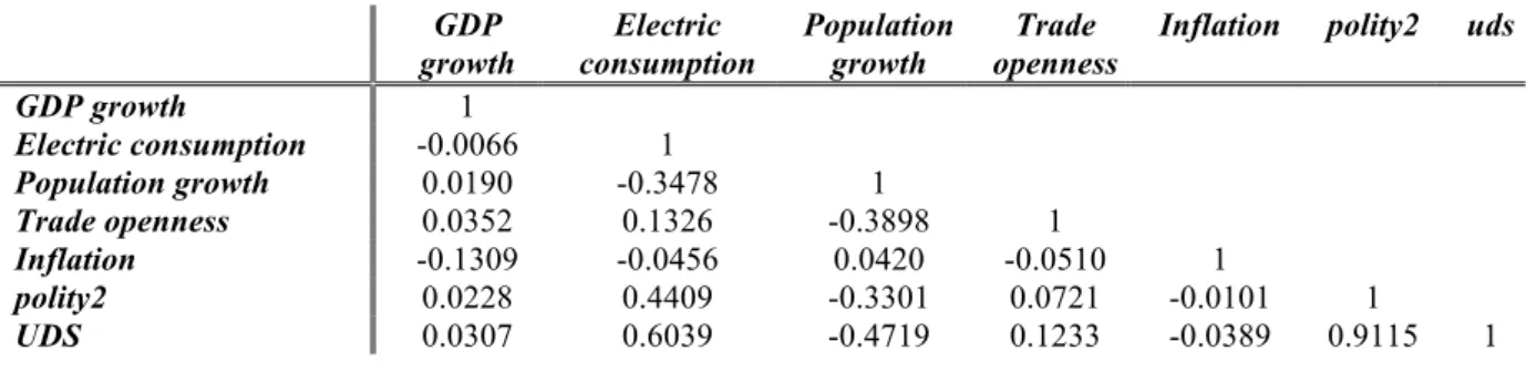
Table 3. Variance co-variance matrix
GDP growth
Electric consumption
Population growth
Trade openness
Inflation polity2 uds
GDP growth 1
Electric consumption -0.0066 1
Population growth 0.0190 -0.3478 1
Trade openness 0.0352 0.1326 -0.3898 1
Inflation -0.1309 -0.0456 0.0420 -0.0510 1
polity2 0.0228 0.4409 -0.3301 0.0721 -0.0101 1
UDS 0.0307 0.6039 -0.4719 0.1233 -0.0389 0.9115 1
From table 3, it is difficult not to take special notice of the very high correlation between polity2
and UDS – this should be a good sign, since they are meant to measure the same phenomenon.
Conclusions must be taken with care, however, since polity2’s non-stationarity could mean that
this correlation is spurious.
V. Methodology
According to the discussion in section III, we chose to follow Gerring et al. (2005) by using a
measure of “political stock” – henceforth defined as political capital (or pk) – as our indicator for
democracy. This variable is constructed as a stock of all “flows of democracy” (the polity2 and
UDS variables) up till time t, with a 1% yearly depreciation10. Since political capital depreciation
is a somewhat novel concept, the way we postulate it leaves room for discussion. We identify
three possibilities:
a) No depreciation (pk0);
b) Depreciation towards 0 (pk1) (“neutral”, neither democratic nor autocratic);
c) Depreciation towards -10 (pk2).
The three possibilities are detailed in table 4.
10
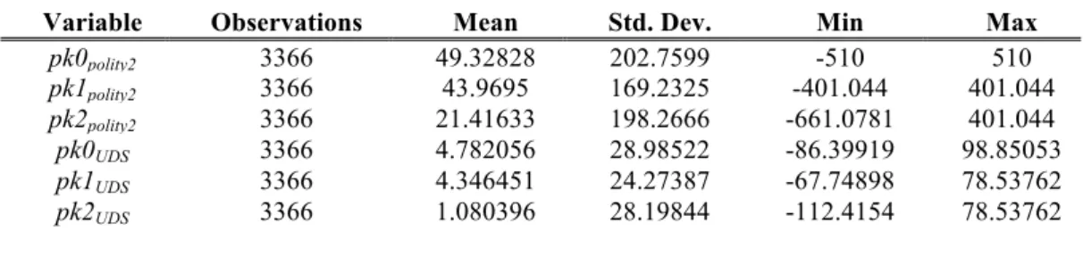
Table 4. Descriptive statistics for pk0, pk1 and pk2
Variable Observations Mean Std. Dev. Min Max
pk0polity2 3366 49.32828 202.7599 -510 510
pk1polity2 3366 43.9695 169.2325 -401.044 401.044
pk2polity2 3366 21.41633 198.2666 -661.0781 401.044
pk0UDS 3366 4.782056 28.98522 -86.39919 98.85053
pk1UDS 3366 4.346451 24.27387 -67.74898 78.53762
pk2UDS 3366 1.080396 28.19844 -112.4154 78.53762
For us to choose a), we would be assuming that a democracy flow would have the same impact
on all subsequent years. This does not seem a very realistic postulation – it makes sense that the
impact of an occurrence that increases the level of democracy subsides across time (democracy
requires sustained efforts). As such, we cast pk0 aside.
pk1 assumes that both democracies and dictatorships tend to converge to a “grey zone” – neither
democratic nor autocratic. pk2, on the other hand, assumes that any regime tends do degenerate
towards autocracy. The main difference between the two is the conceptualization of democracy:
while pk1 reveals the vision that dictatorship and democracy are different articles that both tend
to subside if not “renewed” (towards each other, due to the nature of our variable), pk2 rather
formulates dictatorship as the absence of democracy – depreciation, as such, is always negative.
Democratization (anti-autocratization) efforts are lost along time if not renewed. While we have
found it hard to choose between these two indicators, there is an obvious mathematical
advantage to pk1 – it converges to zero, while pk2 may decrease infinitely if a given country
accumulates too much negative political capital. This is not a very realistic situation – we would
effectively be condemning a country under a long dictatorship to ever-decreasing political
capital. Due to this and to the fact that Gerring et al. seem to follow the pk1 scheme11, we choose
this option as well (henceforth referred to simply as pk). Im-Pesaran-Shin unit root tests to both
the pk1 variables reject the null hypothesis of the existence of unit roots12.
We construct, as such, our political capital variable in the following manner:
11 It is not made absolutely clear. 12
When demeaned, p-values are 0.0000 for both polity2 and UDS. 𝑝𝑘1!"#$%&! and 𝑝𝑘1!"# display a correlation of
𝑝𝑘!,! = 0.99∗𝑝𝑘!,!!!+𝑝𝑓!,! (𝐼)
where 𝑝𝑘!,! is the stock of political capital of country i at time t and 𝑝𝑓!,! is the political flow of
country i at time t13.
Since our data start in 1960, our political capital accumulation begins in this year. Using a
broader timeframe (Gerring et al. start in 1900, although this choice is arbitrary) would imply
making assumptions on missing values of the flow variables, which could compromise our
estimation’s validity – we chose, as such, to stick with data that was entirely available.
It is worthy of notice how novel this approach is – other than Gerring et al., the concept political
capital has, as far as we could find, only been used by Persson and Tabellini (2006), who follow
a similar postulation, augmented with neighboring political effects.
As for the estimation itself, we follow a simple two-step process. Firstly, due to the structure of
our data (higher number of countries than number of years) and the presence of a lag of the
dependent variable on the right-hand side of the regression, we use the Arellano-Bond estimator
(Arellano and Bond, 1991), in line with literature such as Acemoglu et al. (2014), to run a
regression with our dependent variable, economic growth, and all controls:
𝑔𝑟𝑜𝑤𝑡ℎ!,!= 𝛼+𝛽𝑔𝑟𝑜𝑤𝑡ℎ!,!
!! +γX!,!+𝑇𝐷!+𝜀!,! (𝐼𝐼)
where 𝛼 is an intercept term, 𝑔𝑟𝑜𝑤𝑡ℎ!,! is the GDP growth of country i at time t, X!,! is a vector
of controls for country i at time t, 𝑇𝐷! is a full set of year dummies and 𝜀!,! are the residuals. This
error term represents “controlled” growth – since our objective is to build a graph that relates
growth to political capital, we then use the estimated residuals from (II) to perform a second
estimation, this time via OLS with fixed country effects and clustered standard errors, so as to
avoid concerns with heteroskedasticity:
𝜀!
,! =𝛼+𝛽𝑝𝑘!,!!!+𝛾𝑝𝑘!!,!!!+𝜂𝑝𝑘!,!!!
!
+𝜃𝑝𝑘!
,!!!
! +𝜙𝑝𝑘!,!
!!
! +
𝜓𝑝𝑘!,!!!
! +𝑢
!,! (𝐼𝐼𝐼)
where 𝑢!,! is the error term. With the inclusion of the pk term to the power of 1 to 614, we aim to
make sure that we do not miss any non-linearity. We intend on performing various estimations of
(III) with an increasing number of exponential terms, in order to evaluate which is the most
adequate. In line with Gerring et al. and the general literature, we use political capital with a
one-year lag. Finally, from (III) we predict 𝜀!,! and plot it against 𝑝𝑘!,!
!!, so as to obtain our curve.
The idea behind the separation of regressions (II) and (III) is to obtain a final function in only
two variables, in order to facilitate graphical depiction.
VI. Results
We begin this section by running and comparing several specifications, so as to ascertain which
one is the most adequate. We are aware that our method assumes orthogonality between the
political capital variables and all controls, effectively meaning that our estimated curves may not
be entirely precise. For this reason, the specification tests are made with a “complete” equation
(II), to which we add the political capital variables. Tables 5 and 6 present estimation results for
this model with the various possible numbers of exponential terms.
14
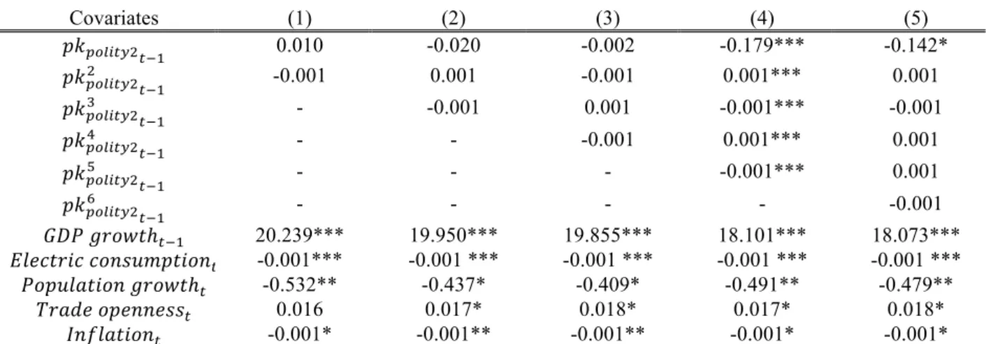
Table 5. Specification tests for polity2 (dependent variable: 𝑮𝑫𝑷𝒈𝒓𝒐𝒘𝒕𝒉𝒕)
Covariates (1) (2) (3) (4) (5)
𝑝𝑘!"#$%&!!!! 0.010 -0.020 -0.002 -0.179*** -0.142*
𝑝𝑘!"#$%&! !
!!! -0.001 0.001 -0.001 0.001*** 0.001
𝑝𝑘!"#$%&! !
!!! - -0.001 0.001 -0.001*** -0.001
𝑝𝑘!"#$%&! !!!! - - -0.001 0.001*** 0.001
𝑝𝑘!"#$%&! !
!!! - - - -0.001*** 0.001
𝑝𝑘!"#$%&!
!
!!! - - - - -0.001
𝐺𝐷𝑃𝑔𝑟𝑜𝑤𝑡ℎ!
!! 20.239*** 19.950*** 19.855*** 18.101*** 18.073*** 𝐸𝑙𝑒𝑐𝑡𝑟𝑖𝑐𝑐𝑜𝑛𝑠𝑢𝑚𝑝𝑡𝑖𝑜𝑛! -0.001*** -0.001 *** -0.001 *** -0.001 *** -0.001 ***
𝑃𝑜𝑝𝑢𝑙𝑎𝑡𝑖𝑜𝑛𝑔𝑟𝑜𝑤𝑡ℎ! -0.532** -0.437* -0.409* -0.491** -0.479**
𝑇𝑟𝑎𝑑𝑒𝑜𝑝𝑒𝑛𝑛𝑒𝑠𝑠! 0.016 0.017* 0.018* 0.017* 0.018*
𝐼𝑛𝑓𝑙𝑎𝑡𝑖𝑜𝑛! -0.001* -0.001** -0.001** -0.001* -0.001* Notes: this table reports estimates of the effect of each independent variable on GDP growth for the Arellano-Bond estimation of each model. Coefficients are multiplied by 100 and rounded to 3 decimal places. All estimations contain a full set of year dummies (omitted in this table). Number of observations: 2302. * denotes significance at a 10% level, ** at a 5% level and *** at a 1% level. Tests for autocorrelation of order 2, 4 and 5 show no evidence of autocorrelation. There is evidence for autocorrelation of order 3 at a 10% confidence level, meaning that our estimated standard errors may be biased downwards. To curb this issue, robust standard errors are employed.
Table 6. Specification tests for UDS (dependent variable: 𝑮𝑫𝑷𝒈𝒓𝒐𝒘𝒕𝒉𝒕)
Covariates (6) (7) (8) (9) (10)
𝑝𝑘!"#!!! 0.010 -0.258*** -0.236* -0.417*** -0.570*
𝑝𝑘!"#! !
!! -0.001 0.004*** 0.003 0.012 0.022
𝑝𝑘!"#! !
!! - -0.001*** -0.001 -0.001 -0.001
𝑝𝑘!"#!
!!! - - -0.001 0.001 0.001
𝑝𝑘!"# !
!!! - - - -0.001 -0.001
𝑝𝑘!"# !
!!! - - - - 0.001
𝐺𝐷𝑃𝑔𝑟𝑜𝑤𝑡ℎ!
!! 20.280*** 19.847*** 19.842*** 19.856*** 19.849***
𝐸𝑙𝑒𝑐𝑡𝑟𝑖𝑐𝑐𝑜𝑛𝑠𝑢𝑚𝑝𝑡𝑖𝑜𝑛! -0.001*** -0.001*** -0.001*** -0.001*** -0.001***
𝑃𝑜𝑝𝑢𝑙𝑎𝑡𝑖𝑜𝑛𝑔𝑟𝑜𝑤𝑡ℎ! -0.531** -0.455* -0.452* -0.490** -0.486**
𝑇𝑟𝑎𝑑𝑒𝑜𝑝𝑒𝑛𝑛𝑒𝑠𝑠! 0.016* 0.018* 0.018* 0.018* 0.018*
𝐼𝑛𝑓𝑙𝑎𝑡𝑖𝑜𝑛! -0.001** -0.001** -0.001** -0.001** -0.001**
Notes: this table reports estimates of the effect of each independent variable on GDP growth for the Arellano-Bond estimation of each model. Coefficients are multiplied by 100 and rounded to 3 decimal places. All estimations contain a full set of year dummies (omitted in this table). Number of observations: 2302. * denotes significance at a 10% level, ** at a 5% level and *** at a 1% level. Tests for autocorrelation of order 2, 4 and 5 show no evidence of autocorrelation. There is evidence for autocorrelation of order 3 at a 10% confidence level, meaning that our estimated standard errors may be biased downwards. To curb this issue, robust standard errors are employed.
Firstly, all but one instance of our used control variables display statistical significance, and
additionally they also present very similar estimated coefficients in all formulations (both for
polity2 and UDS). All signs are what we would expect: positive for the lag of GDP growth,
indicating some persistence; negative for electric consumption, in accordance with the theory of
IV; positive for trade openness, emphasizing the positive effects of trade on growth and finally
negative for inflation, in line with Barro (1995).
Table 5 shows estimation results for the various possible specifications using the polity2
variable. We find extremely high significance for specification (4), and basically no significance
for all other ones – it is, hence, quite easy to choose between them. We find, with these results,
our first concrete evidence that the relationship between democratic evolution in a society and its
economic growth should not be linear – the polity2 variable predicts the existence of four
inflexion points.
Table 6, on the other hand, displays results for the same specifications, using the UDS variable.
We again find full (and quite high) significance for only one specification – this dataset predicts
that (7) is the most adequate postulation, meaning 2 inflexion points. With this result, we add
robustness to our recent non-linearity conclusion. It is worthy of note that the inverted-U-shaped
relationship that some literature has found does not seem to occur with a political capital
variable.
The next step lies in the estimation of the actual curves, using the two-step process described in
section V. We omit the estimation results, since they should be less precise than the ones
presented. Below, we present the curves that correspond to specifications (4) (table 5) and (7)
(table 6), since these are the ones that display full significance. In appendix A2, all remaining
curves are presented, showing the sensitivity of the curve’s shape to differences in specification
– the UDS ones display high consistency, while the polity2 curves are somewhat more diverse in
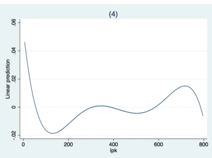
Figure 1. Graphical depiction of specification (4)
Notes: the y-axis measures the predicted residuals from equation (II), while the x-axis measures the stock of political capital (built with the polity2 variable).
Figure 2. Graphical depiction of specification (7)
Notes: the y-axis measures the predicted residuals from equation (II), while the x-axis measures the stock of political capital (built with the UDS variable).
Prior to any interpretation, it is useful to recall that the y-axis values are predicted residuals – as
such, a negative value does not necessarily imply negative GDP growth (simply lower than what
Both figure 1 and 2 add weight to the argument that the relationship we want to model is
non-linear. Actually, they are quite similar in broad terms and implications – they both imply that
maximum growth is attained with minimum democracy stock and that there is a “democracy
maximum”, a point that corresponds to a quite high level of political capital that maximizes
growth. Two main facts are worthy of notice about this point – firstly, it implies lower growth
than the total dictatorship point; secondly, it does not occur for the maximum observed value of
political capital. This not only backs the literature that argues that dictatorships may be growth
maximizing (“Growth-friendly dictatorships”, De Luca et al., 2015), it also says that
democratization does not always mean increased economic growth – from a certain point
onwards, when a society furthers its democratization process, it is sacrificing some growth.
Eventually, democracy becomes a “good-to-have”. If we assume agents know this relationship15,
it means that, at least from the democracy maximum onwards, people value their welfare above
economic growth.
While not as blatant as their similarities, these curves also display a few differences. The most
striking one is probably optimism – the UDS curve is expressively more optimistic on how close
the democracy maximum is to total dictatorship in terms of growth. Actually, it is nearly the
same, while polity2 predicts less than half the growth the economy would experience if it had
zero political capital.
Since these curves measure cumulative democratic experience along the x-axis, they depict the
democratization path of a theoretical country from complete autocracy to a developed democracy
status. Their conclusions are, in our opinion, both interesting and controversial – society has an
economically demanding path to tread in its democratization process. While we did not make
any effort to, our results somewhat support the theory that some poor countries may not be
15
economically ready for democracy – democratization could cripple their economy, possibly to
the point where regime reversals could occur.
It should be noted, to finalize, that all we see in the curve is the impact of democratization on
growth. It is entirely possible that, at any point, other factors (our controls, for example) offset
any growth gains or losses created by the political process. Although we believe this to be a quite
important relationship, one should be aware of its ceteris paribus environment.
VII. Robustness
Since we have estimated our section VI models with two different democracy measures, we have
already performed a significant robustness test to our main results. This section will, as such,
serve to perform an estimation that is more in line with the remaining literature – notably, using
democracy flows rather than a stock. We have, in section IV, found that the polity2 variable, as a
flow, displays a unit root – due to this and the fact that estimations akin to ours using variables
from the Polity IV project abound in the literature, we will use UDS for this section16. This will
both allow us to understand if conclusions change when we swap between formulations and how
UDS behaves when used as a flow (specifically, if it backs the conclusions the literature has
reached using the Polity IV project’s variables). It is important to notice, however, that the
specifications in this section do not measure the same as those in section VI – while political
capital measures the maturity of a country’s democracy, the following specifications measure the
impact on growth of the level of democracy of the country under analysis at a given year. We
have tested both 10-year and 5-year lags17 of the democracy variable in our specifications,
having obtained similar results. Since the latter are slightly more significant and it seems very
16
Were we to ignore this and use our database to perform this section’s estimation with the polity2 flows, we would find significance for one, two and three inflexion points, all obtaining the inverted-U-shaped curve Barro (1996) and Alfano and Baraldi (2016) estimate.
17
reasonable to us that democratization could impact economic growth in five years, we present
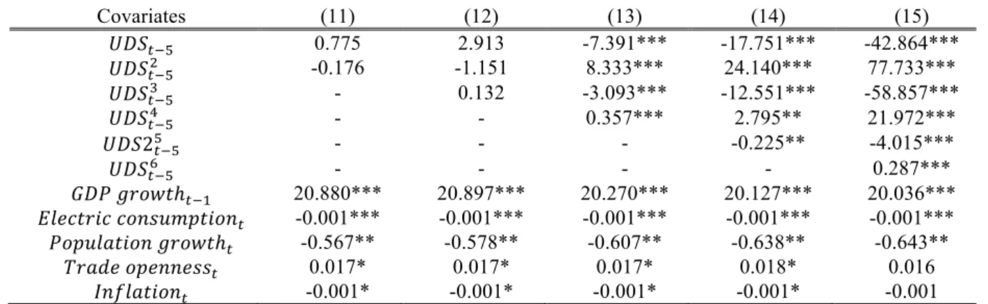
estimation results for the model with 5-year lagged democracy flows.
Table 7. Specification tests for UDS flows (dependent variable: 𝑮𝑫𝑷𝒈𝒓𝒐𝒘𝒕𝒉𝒕)
Covariates (11) (12) (13) (14) (15)
𝑈𝐷𝑆!
!! 0.775 2.913 -7.391*** -17.751*** -42.864***
𝑈𝐷𝑆! !!
! -0.176 -1.151 8.333*** 24.140*** 77.733***
𝑈𝐷𝑆! !!
!
- 0.132 -3.093*** -12.551*** -58.857***
𝑈𝐷𝑆! !!
! - - 0.357*** 2.795** 21.972***
𝑈𝐷𝑆2!
!!
! - - - -0.225** -4.015***
𝑈𝐷𝑆! !!
! - - - - 0.287***
𝐺𝐷𝑃𝑔𝑟𝑜𝑤𝑡ℎ!
!! 20.880*** 20.897*** 20.270*** 20.127*** 20.036***
𝐸𝑙𝑒𝑐𝑡𝑟𝑖𝑐𝑐𝑜𝑛𝑠𝑢𝑚𝑝𝑡𝑖𝑜𝑛! -0.001*** -0.001*** -0.001*** -0.001*** -0.001***
𝑃𝑜𝑝𝑢𝑙𝑎𝑡𝑖𝑜𝑛𝑔𝑟𝑜𝑤𝑡ℎ! -0.567** -0.578** -0.607** -0.638** -0.643**
𝑇𝑟𝑎𝑑𝑒𝑜𝑝𝑒𝑛𝑛𝑒𝑠𝑠! 0.017* 0.017* 0.017* 0.018* 0.016
𝐼𝑛𝑓𝑙𝑎𝑡𝑖𝑜𝑛! -0.001* -0.001* -0.001* -0.001* -0.001
Notes: this table reports estimates of the effect of each independent variable on GDP growth for the Arellano-Bond estimation of each model. Coefficients are multiplied by 100 and rounded to 3 decimal places. All estimations contain a full set of year dummies (omitted in this table). Number of observations: 2243. * denotes significance at a 10% level, ** at a 5% level and *** at a 1% level. Tests for autocorrelation of order 2, 4 and 5 show no evidence of autocorrelation. There is some evidence (not in all specifications) for autocorrelation of order 3 at a 10% confidence level, meaning that our estimated standard errors may be biased downwards. To curb this issue, robust standard errors are employed.
Table 7 is very suggestive of a complex non-linear relationship between democracy flows and
future growth – our fully significant specifications (13), (14) and (15) imply 3, 4 or 5 inflexion
points, respectively. Figure 3 depicts these three regressions:
Figure 3. Graphical depiction of specifications (13) (left), (14) (center) and (15) (right)
Notes: the y-axis measures the predicted residuals from equation (II), while the x-axis measures the stock of political capital (built with the UDS variable).
As figure 3 shows, the three possibilities are, graphically, very similar. It is striking how they
differ from the Barro (1996) and Alfano and Baraldi (2016) results – they display a U-shaped
curve rather than their inverted U. In terms of implications, they somewhat resemble figures 1
difference here is that now, with curves (13) and (14), from a certain, high-democracy point
onwards, democratization does increase growth. On average, the most “growth-unfriendly”
points are those in the middle of the spectrum, while very high or very low flows appear to
maximize economic growth. In a nutshell, we conclude that zero or close to zero democracy
should cause growth (again), and also that a democratic flow needs to be sufficiently high to
have the best impact on economic performance.
While it is undeniably true that this curve estimates something different from figures 1 and 2,
one conclusion is clearly backed by both sections’ estimations – the relationship between
economic growth and democracy should not be regarded as linear.
While this section has helped to draw further interesting conclusions, we emphasize that we do
not think this kind of specification (the use of democratic flows) is the most adequate to study
democracy and growth. In this section, we find that, on average, there is a level of democracy
flow that maximizes growth, but if our section VI estimation is to be trusted, this will, for each
country, depend on its current democratic position – if it is sufficiently low or past the
democracy maximum the flow that maximizes growth should be negative, and if it is sufficiently
close to (but before) the democracy maximum it should be positive. This is the reason why we
believe that performing this kind of flow analysis for this specific question is not the most
correct approach.
VIII. Concluding remarks
Along the course of this paper, we have shown that the relationship between a society’s
democratization level and its economic growth should be non-linear, meaning that the impact of
further democratization on economic performance should vary depending on each country’s
initial stock of democracy. We provide an in-depth discussion on the concept of democracy
and those similar. Our conclusions, however, are robust to the use of democracy flow analysis,
the approach that the large majority of the literature uses.
Via the use of two different measures of democracy, the widely used polity2 variable by the
Polity IV project and the Unified Democracy Scores by Pemstein et al. (2010), we have further
provided insightful comparison between these two measures, creating a new avenue through
which we add to the literature. We also coin the term “democracy maximum”, which represents
the level of democratic development that is enough to classify a country as an evolved
democracy and maximizes economic growth. Finally, we add some weight to the argument that
autocracies may maximize growth by finding that our maximum estimated economic growth
occurs with zero political capital.
Our work leaves, in our view, several open paths for improvement and further investigation,
notably the use of a larger timeframe (especially for the accumulation of the political stock) and
a more balanced panel, more sophisticated econometric techniques and alternative political
capital formulations. The crossing of these results with a measure of general population welfare,
so as to measure the net gains from democratization (economic versus social, potentially) could
also yield an interesting further research question. Finally, democracy stock and flow analysis
could be combined in a single regression framework to evaluate the impact of flows when
References
Acemoglu, Daron. 2008. “Oligarchic Versus Democratic Societies.” Journal of the European
Economic Association 6(1): 1-44.
Acemoglu, Daron; Naidu, Suresh; Restrepo, Pascual; Robinson, James A.. 2014.
“Democracy Does Cause Growth.” National Bureau of Economic Research: Working Paper 20004.
Alfano, Maria Rosaria; Baraldi, Anna Laura. 2016. “Democracy, Political Competition and Economic Growth.” Journal of International Development 28: 1199-1219.
Arellano, Manuel; Bond, Stephen. 1991. “Some Tests of Specification for Panel Data: Monte
Carlo Evidence and an Application to Employment Equations.” The Review of Economic
Studies 58(2): 277-297.
Barro, Robert J.. 1995. “Inflation and Economic Growth.” National Bureau of Economic
Research: Working Paper 5326.
Barro, Robert J.. 1996. “Democracy and Growth.” Journal of Economic Growth 1: 1-27.
Campbell, David F.J.. 2008. “The Basic Concept for the Democracy Ranking of the Quality of
Democracy.” Vienna: Democracy Ranking.
Campbell, David F.J.; Pölzbauer, Georg. 2008. “The Democracy Ranking 2008 of the Quality
of Democracy: Method and Ranking Outcome.” Vienna: Democracy Ranking.
Clague, Christopher; Keefer, Philip; Knack, Stephen; Olson, Mancur. 1996. “Property and
Contract Rights in Autocracies and Democracies.” Journal of Economic Growth 1: 243-276.
Coccia, Mario. 2010. “Democratization is the driving force for technological and economic change.” Technological Forecasting & Social Change 77: 248-264.
Corujo, Sara A.; Simões, Marta C. N.. 2012. “Democracy and Growth: Evidence for Portugal
(1960-2001).” Transition Studies Review 18: 512-528.
Davis, Lewis S.. 2010. “Institutional flexibility and economic growth.” Journal of Comparative
Economics 38: 306-320.
De Luca, Giacomo; Litina, Anastasia; Sekeris, Petros G.. 2015. “Growth-friendly
dictatorships.” Journal of Comparative Economics 43: 98-111.
Doucouliagos, Chris; Ulubaşoğlu, Mehmet Ali. 2006. “Economic freedom and economic growth: Does specification make a difference?” European Journal of Political Economy 22: 60-81.
Foldvari, Peter. 2014. “A latent democracy measure 1850-2000.” Centre for Global Economic
History: Working paper no. 59.
Gerring, John; Bond, Phillip; Barndt, William T.; Moreno, Carola. 2005. “Democracy and
Economic Growth: A Historical Perspective.” World Politics 57: 323-364.
Helliwell, John F.. 1994. “Empirical Linkages between Democracy and Economic Growth.” British Journal of Political Science 24(2): 225-248.
Knutsen, Carl Henrik. 2011. “Democracy, Dictatorship and Protection of Property Rights.”
The Journal of Development Studies 47(1): 164-182.
Knutsen, Carl Henrik. 2012. “Democracy and economic growth: A survey of arguments and results.” International Area Studies Review 15(4): 393-415.
Knutsen, Carl Henrik. 2015. “Why Democracies Outgrow Autocracies in the Long Run: Civil
Liberties, Information Flows and Technological Change.” KYKLOS 68(3): 357-384.
Krieckhaus, Jonathan. 2006. “Democracy and Economic Growth: How Regional Context
Influences Regime Effects.” British Journal of Political Science 36(2): 317-340.
Leblang, David A.. 1996. “Property Rights, Democracy and Economic Growth.” Political
Research Quarterly 49(1): 5-26.
Madsen, Jakob B.; Raschky, Paul A.; Skali, Ahmed. 2015. “Does democracy drive income in
Marshal, Monty G.; Gurr, Ted Robert; Jaggers, Keith. 2016. “Polity IV Project: Political Regime Characteristics and Transitions, 1800-2015. Dataset Users’ Manual.” Center for
Systemic Peace.
Mauro, Paolo. 1995. “Corruption and Growth.” The Quarterly Journal of Economics 110(3): 681-712.
Murtin, Fabrice; Wacziarg, Romain. 2014. “The democratic transition.” Journal of Economic
Growth 19: 141-181.
Olson, Mancur. 1993. “Dictatorship, Democracy, and Development.” American Political
Science Review 87(3): 567-576.
Pemstein, Daniel; Meserve, Stephen A.; Melton, James. 2010. “Democratic Compromise: A
Latent Variable Analysis of Ten Measures of Regime Type.” Political Analysis 18: 426-449.
Persson, Torsten; Tabellini, Guido. 2006. “Democratic Capital: The Nexus of Political and Economic Change.” National Bureau of Economic Research: Working Paper 12175.
Tavares, José; Wacziarg, Romain. 2001. “How democracy affects growth.” European
Economic Review 45: 1341-1378.
Treier, Shawn; Jackman, Simon. 2008. “Democracy as a Latent Variable.” American Journal
of Political Science 52(1): 201-217.
Vanhanen, Tatu. 2002. “Polyarchy Dataset Manuscript.” International Peace Research
Appendix
A1. Included countries and their respective polity2 and UDS scores, 1960 and 2010
1960 2010
Country polity2 UDS polity2 UDS
Albania -9 -1.16 9 0.47
Argentina -1 0.05 8 0.66
Australia 10 1.19 10 2.25
Austria 10 1.31 10 1.69
Belgium 10 1.3 8 1.35
Bolivia -3 -0.01 7 0.32
Brazil 6 0.44 8 0.92
Bulgaria -7 -0.98 9 0.81
Cameroon -6 -0.21 -4 -0.49
Canada 10 1.08 10 1.77
Sri Lanka 7 0.69 4 0.24
Chile 5 0.48 10 1.18
China -8 -1.08 -7 -0.77
Colombia 7 0.21 7 0.34
Congo, DRC 0 -0.44 5 -0.43
Costa Rica 10 0.96 10 1.41
Denmark 10 1.31 10 2.23
Dominican Republic -9 -1.17 8 0.61
Ecuador 2 0.33 5 0.3
Finland 10 1.3 10 2.24
France 5 0.45 9 1.09
Ghana -8 -0.77 8 0.67
Greece 4 0.36 10 1.26
Guatemala -5 -0.23 8 0.38
Hungary -7 -0.97 10 1.18
India 9 0.84 9 0.83
Ireland 10 1.09 10 1.48
Israel 10 1.18 10 1.17
Italy 10 1.59 10 1.17
Cote d'Ivoire -9 -0.91 0 -0.47
Jamaica 10 1.45 9 0.74
Japan 10 1.2 10 1.38
Jordan -9 -1.08 -3 -0.51
South Korea 8 0.21 8 1.07
Madagascar -1 0.14 0 -0.39
Malaysia 10 0.44 6 0.35
Mali -7 -0.67 7 0.42
Mexico -6 -0.3 8 0.56
Morocco -5 -0.76 -6 -0.47
Oman -10 -1.87 -8 -0.9
Netherlands 10 1.53 10 1.7
New Zealand 10 1.18 10 1.88
Niger -7 -0.67 3 -0.29
Nigeria 8 0.41 4 -0.15
Norway 10 1.18 10 2.26
Pakistan -7 -1.14 6 0.02
Peru 5 0.11 9 0.66
Philippines 5 0.48 8 0.56
Poland -7 -0.98 10 1.18
Portugal -9 -1 10 1.48
Romania -7 -0.98 9 0.71
Saudi Arabia -10 -1.62 10 -1.5
Senegal -1 -0.32 7 0.28
South Africa 4 -0.24 9 0.8
Spain -7 -1.2 10 1.55
Sweden 10 1.18 10 2.25
Switzerland 10 1.09 10 2.26
Thailand -7 -0.98 4 0.2
Tunisia -9 -0.62 -4 -0.64
Turkey 7 -0.39 7 0.33
Egypt -7 -0.8 -3 -0.51
United Kingdom 10 1.18 10 1.56
United States 10 1.08 10 1.56
Burkina Faso -7 -1 0 -0.29
Uruguay 8 0.85 10 1.56
A2. Tables 5 and 6: graphical depictions of specifications (1) to (10)
Notes: the y-axis measures the predicted residuals from equation (II), while the x-axis measures the stock of political capital (polity2 for the left-hand-side graphs and UDS for the right-hand-side ones).
-.
0
1
-.
0
0
5
0
.005
.01
.015
L
in
e
a
r
p
re
d
ict
io
n
0 200 400 600 800
lpk