ABSTRACT: Integrated pest management programs for soybean (Glycine max (L.) Merrill) must be based on efficient sampling plans for estimating the pest population. Based on the spatial distribution of the Neotropical brown stink bug Euschistus heros (Fabricius, 1794) found on soybean, it was possible to construct a sequential sampling plan for the survey of this insect found on soybean. The experiment was carried out during two growing seasons, 2010/2011 and 2011/2012, using the transgenic soybean cultivar M 7908 RR, in plots of 10,000 m2 subdivided into 100 plots of 100 m2 (10 m × 10 m). Nymphs > 0.5 cm (4th and 5th instars) plus adults were counted weekly from five drop cloth technique samplings per plot. To evaluate insect dispersion in the area, the following indices were used: variance/mean ratio, Morisita’s index, Green’s coefficient, the k exponent of the negative binomial distribution, and estimation of the common exponent k (kc). To study probabilistic models to describe the spatial distribution of the insects, adjustments of the Poisson and negative binomial distributions were tested. Two sequential sampling plans for separate fields, one for grain production and the other for seed production, were prepared.The data fitted a negative binomial distribution and a sampling plan was drawn up using the sequential likelihood ratio test (SLRT). The maximum sampling unit number expected for control-related decision making was six in grain production fields, and nine in seed production fields.
Keywords: Neotropical brown stink bug, sampling method
Introduction
The Neotropical brown stink bug Euschistus heros (Fabricius, 1794) (Heteroptera: Pentatomidae) is a prominent pest of soybean (Glycine max (L.) Merrill) in Brazil (Sosa-Gómez and Silva, 2010). This pentatomid is largely responsible for the reduction in quality and weight of seeds (Corrêa-Ferreira and Azevedo, 2002).
The distribution of E. heros has increased in the past five years and, due to its increased populations, most insecticide applications are designed accordingly to manage this pest (Sosa-Gómez and Silva, 2010). However, populations of this pentatomid are difficult to manage using organophosphates (methamidophos, acephate, chlorpyrifos, and monocrotophos) or cyclodiene endosulfan (Sosa-Gómez et al., 2009). Consequently, control strategies are based on spraying using a limited group of insecticides (Sosa-Gómez et al., 2001).
Management of arthropod populations requires quick and efficient sampling of pests and their natural enemies to ensure the success and efficiency of the control methods (Fernandes et al., 2003). The conventional sampling methods for pests are based on a fixed number of sampling units (Kogan and Herzog, 1980); nevertheless, sequential sampling is an alternative that has been considered faster and reliable (Fernandes et al., 2003).
In sequential sampling, the number of sample units per area is variable, which helps in reducing the time spent on sampling and decreasing production costs without losing the sampling reliability for decision making. Further, the units are examined in sequence until decisions can be made based on the accumulated data as
to whether the results should be accepted or rejected, or whether sampling should be continued (Barbosa, 1992). This study aimed to establish a sequential sampling plan for E. heros in soybean.
Materials and Methods
The experiment was carried out in Jaboticabal, in the state of São Paulo, Brazil (21°14'05" S 048º17'09" W; 615 m a.s.l.), for two growing seasons, 2010/2011 and 2011/2012. The soybean cultivar M 7908 RR (transgenic with tolerance to the herbicide glyphosate), which is an early-maturing cultivar, was used. Seeds were sown on Nov 24th 2010, and plants emerged on Nov 29th 2010.
For the second cropping season, seeds were sown on Nov 21st 2011, emerging on Nov 26th 2011, when the
applications of herbicide (Fomesafen+Fluazifop-p-butyl) and fungicide (azoxistrobina+ciproconazole) were administered. In both growing seasons, a commercial soybean field of 30 ha in area was chosen, in which a 10,000 m² area was defined and then subdivided into 100 plots of 100 m² each (10 × 10 m). Each plot was considered a sampling unit. The soybean was planted in 45-cm plant spacing, making 330,000 plants in total. Insecticides were not sprayed during the experiment to avoid any interference with the entomofauna.
Weekly samplings were conducted from day 86 on to day 115 after plant emergence (DAE), which corresponded to the early stages of seed filling (R5) to full maturity (R8) (Fehr and Caviness, 1977). Five sampling points per unit (100 m2) were randomly assessed using
the drop cloth technique, which is a method requiring a 1São Paulo State University/FCAV – Dept. of Phytosanitary,
Via de Acesso Prof. Paulo Donato Castellane s/n – 14884-900 – Jaboticabal, SP – Brazil.
2São Paulo State University/FCAV – Dept. of Exact Science. *Corresponding author <[email protected]>
Edited by: Richard V. Glatz
Sequential sampling of
Euschistus heros
(Heteroptera: Pentatomidae) in soybean
Leandro Aparecido de Souza1, José Carlos Barbosa2*, José Fernando Jurca Grigolli1, Diego Felisbino Fraga1, Lílian Cristina
Moraes2, Antonio Carlos Busoli1
white piece of cloth or plastic, 1 m in length and 0.5 m in width, to be attached to two wooden sticks that are placed in between two rows of soybean plants. Plants should be shaken so that the pests will fall down onto the cloth. Accordingly, 30 plants were sampled, since each row of plants contained approximately 15 plants. At each sampling point, the number of nymphs > 0.5 cm (4th and 5th instars) plus adults was recorded since
soybean seeds are susceptible to injury and damage caused during these stages of insect development, which in turn inform decisions on the application of pesticides (Hoffmann-Campo et al., 2000).
For data analysis, the average values and variance in the number of nymphs > 0.5 cm plus adults per plot were recorded for each sampling period. The dispersion indices for determining the degree of aggregation of E. heros were calculated, as follows:
Variance/mean ratio (I):The variance/mean ratio, also called the dispersion index (I = s2 m–1), is commonly
used to measure the deviation of an arrangement in ran-dom conditions, in which I = 1 indicates a ranran-dom spa-tial distribution; I < 1 uniform distribution; and I > 1 aggregated distribution (Rabinovich, 1980). The distance of randomness can be tested by using the chi-square test, with n-1 degrees of freedom [c2= (n-1) s2 m–1] (Elliott,
1979).
Morisita’s index (Id): This index is independent of the size of the sampling unit (Morisita, 1962). This index is given by the equation:
2
2
[ ( 1)]
( 1) ( )
− −
= =
− −
∑
∑
∑
∑ ∑
x x∑
x∑
xId n n
x x x x
where: n = number of sample units; x = number of nymphs or adults per plot.
The Morisita’s index is equal to one for random distributions; greater than one for contagious distributions; and lower than one for regular or uniform distributions. Departure from randomness can be tested by:
2 2
( 1)
( 1) ~ −
=
∑
− + −∑
cd d i i n
X I x n x
If 2 2 (−1 . .; 0,05)
≥ c
d n g l
X the hypothesis of randomness is rejected.
Green’s coefficient (Cx): The Green coefficient is generally used for describing different types of patterns. Negative values indicate a uniform distribution pattern, whereas positive values indicate an aggregate pattern (Green, 1966). It is based on the variance/mean ratio and is given by:
2
1
ˆ ( / ) 1
1
=
− =
−
∑
x n
i i
s m
C
x
where: s² = sampling variance; m = sampling mean; xi = number of nymphs or adults per plot.
The k exponent for negative binomial distribution (k): This index is an indicator of arthropod aggregation, and should only be used when the data fit the negative binomial distribution (Elliott, 1979). Negative values in-dicate a uniform distribution, low and positive values (0 < k < 2) indicate a highly aggregated distribution, val-ues ranging from 2 to 8 indicate a moderate aggregation, and values greater than 8 indicate a random distribution (Costa et al., 2010). Firstly, k values were obtained by the moment's method, which is given by:
2
2
= −
m k
s m,
and later by the maximum likelihood method:
1
ˆ ( )
ln(1 ) ˆ = ˆ
+ =
+
∑
nc ii i
m A x
N
k k x
,
where: N = number of sampling units; A(xi) = sum of frequencies of values greater than xi; nc = number of classes in the frequency distribution; and xi= number of nymphs > 0.5 cm plus adults per plot.
Estimation of the common exponent k (kc): To de-termine a common value of k that represented most of the sampling period, we used the method proposed by Bliss and Owen (1958), known as the “method of weighted regression”. To calculate kc of number of nymphs > 0.5 cm (4th and 5th instars) plus adults, the
samples from two growing seasons were analyzed to-gether.
Probabilistic models for studying the spatial distribution of pests: In each sample, the adjustment of the Poisson and negative binomial distributions was tested. The model shows good adjustment to the original data when the observed and expected frequencies are close. This proximity was tested by the chi-square test, given by:
2 2
1
( )
=
− =
∑
nc i ii i
FO FE
X
FE
,
where: FOi = observed frequency in class i; FEi = expected frequency in class i; nc = number of classes in the frequency distribution.
The number of degrees of freedom of c2 is given
by:
v = nc- np– 1,
Poisson distribution: The Poisson distribution best represents the random spatial distribution of insects and is characterized by presenting the variance equal to the average (s2 = m) (Southwood, 1978). The equations
for calculating the probabilities are given by:
( )
!
−l
l = x
x e P
x
where: P(x) = probability of occurring x individuals in the sampling unit; l = parameter of the distribution (l = m = s2); and e = base of the natural logarithm.
Negative binomial distribution: This index presents the variance as being greater than the average (s2 > µ)
and has two parameters, the average (m) and the expo-nent k (k> 0) (Taylor, 1984). The series of probabilities can be calculated for a sampling by using the following equation:
( 1). .( 1)
( )= P x− R k+ −x , =1, 2, 3, ...
P x x
x ,
in which:
(0) 1
−
= +
k m P
k ,
where: m = sampling mean; k = exponent of the nega-tive binomial distribution; P(x) = probability of occur-ring x individuals in the sampling unit.
The plan was based on the sequential likelihood ratio test (SLRT) proposed by Wald (1945).The plan is to test with the lowest expected number of samples possible in the hypothesis: H0: m = m0 vs. H1: m = m1, where m represents the means and m1 > m0. The rejection of H0 indicates the need to apply pest control methods, while acceptance of H0 means that control is not required (Allen et al., 1972).
The decision straight line equations, which deter-mine whether control is required or not, are called S1 and S0 and are represented by S1 = h1 + an and S0 = h0 + an, in which n indicates the number of sample units to be used, h0 and h1 values are the linear coefficients, and a is the angular coefficient.
Two sequential sampling plans were devised, one for fields of grain and the other for fields used for seed production. For the fields of grain, the control level (m1) at 4.0 nymphs > 0.5 cm plus adults per drop cloth sam-pling and the security level (m0) was set at 1.5 nymph > 0.5 cm plus adults, based on the hypothesis H0: m0 = 1.5 versus H1: m1 = 4.0, and for fields for seed produc-tion the control level (m1) was set at 2.0 nymphs > 0.5 cm plus adults per drop cloth sampling. The security level (m0) was set at 0.75 nymphs > 0.5 plus adults based on the hypothesis H0: m0 = 0.75 versus H1: m1 = 2.0.
The control level (m1) was used in this experi-ment (Hoffmann-Campo et al., 2000) and the security level (m0) was obtained based on the lowest average
found in sampling periods (lower limit) from the seed production field. In the field of grain production, this value was doubled since the level of control was also duplicated. Type I and II errors were determined as a = b = 0.05 which is the most suitable for studies in-volving insects (Young and Young, 1998).
The values of h0, h1 and a were determined ac-cording to the type of spatial distribution of the pest, in this case based on the negative binomial model, using the equations below (Young and Young, 1998):
0
1 0
0 1
1
( )
( )
b
− a
=
+
+
ln h
m m k
ln
m m k
( 0 )
1
1
0 1
1
( )
+
− b
a
=
+
m k
ln h
m ln
m m k
(
)
(
)
1
0
1 0
0 1
+
+
=
+
+
m k
ln
m k
a k
m m k
ln
m m k
where: m0 = security level; m1 = control level; a = type I error; b = type II error; h = auxiliary variable de-pendent p; a = angular coefficient; k = index kc (Com-mon k) calculated by the method proposed by Bliss and Owen (1958).
The test consisted of:
a) Rejection of H0 when the sample size was N* such
that:
aN + h0 < S < aN + h1, for N = 1, 2... N*-1, and
S
≥
aN* + h1b) Acceptance of H0 when the sample size was N*, such
that:
aN + h0 < S < aN + h1, for N = 1, 2, ..., N*-1, and
S
≤
aN* + h0where: N = number of sampling units to be used; S = sum of countings.
In addition to the straight lines, it is convenient to express the characteristic operation curve OC(m), which provides the probability of accepting H0 as a function of the mean m for pre-established values of a and b. In the deduction, Wald (1945) used an auxiliary variable h depending on m, resulting in:
[(1 ) / ] 1
( ) = , 0 [(1 ) / ] [ / (1 )]
− b a − ≠
− b a − b − a
h
h h
OC m h
[(1 ) / ]
( ) = , = 0, = [(1 ) / ] [ / (1 )]
− b a
− b a − b − a
ln
OC m h m a
ln ln
where: a = type I error; b = type II error; h = auxiliary variable dependent p;m = average; a = angular coefficient.
In the negative binomial distributions with k in common, the ratio between h and m is given by:
0 1
1 0 0 1
1 ( / )
= , 0. [( ) / ( ) 1]
− ≠
−
h
h c
q q
m
h
p q p q
k
where: k = exponent k of the negative binomial distribution;h = auxiliary variable dependent p; m = average.
This relationship allows for expressing OC(m) as a function of m, arbitrating h, where k = exponent k of the negative binomial distribution obtained by the maximum likelihood method or the method of moments;
p0 = m0/k; p1= m1/k; q0 = 1 + p0; q1 = 1 + p1.
The curve of the expected size E [N] that provides the mean expected sample size for the decision to accept or reject H0 was calculated for the plan by the expression (Young and Young, 1998):
( ) ( ) [ ] b1 + . OC mb0 b1
E N = , h 0.
m - a
− ≠
where: h = auxiliary variable dependent p;m = average; a = angular coefficient.
By using this function, the expected number of samples can be expressed as a function of m. On the other hand, if in practice it is desirable to fix the sample size, the maximum expected value is recommended for E [N], in the corresponding SLRT.
Results and Discussion
Values for the spatial distribution of nymphs > 0.5 cm plus adults of E. heros for both cropping seasons were greater than one for the variance/mean ratio (I) on six sampling dates, where values were close to one on the other four dates. Thus, the distribution pattern
of the pest ranged from moderately aggregated to random (Table 1). Values for Morisita’s index (Id) are in accordance with those obtained for the variance/mean ratio (Table 1).
Green’s coefficient (Cx) values were positive for all sampling dates and in both cropping seasons (Table 1), indicating aggregated distribution of the pest’s population (Green, 1966). Values for the exponent of negative binomial distribution (k), estimated using the maximum likelihood method, ranged from 0 to 2, which indicates an aggregated pattern; values higher than eight indicate a random distribution (Costa et al., 2010). Immature forms of Nezara viridula (L.) and Piezodorus guildinii (Westw.) at their late stages of development (fourth and fifth instars) are the most important stages for the dispersion of these species in the field (Panizzi et al., 1980).
Initially, data were tested to observe whether they fitted a Poisson distribution; later, since the means were lower than the variances for most of the sampling periods, we tested the data to see if they fitted the negative binomial distribution. Sampling periods demonstrated that their distribution is not random, when chi-square test values were significant at 1 % (114 DAE in growing season 2010/2011 and 115 DAE in growing season 2011/2012) or 5 % probability (94 DAE in growing season 2011/2012) when fitting Poisson’s distribution, (Table 2). When we attempted to fit the sampling periods to the negative binomial distribution, the values were non-significant and lower than the Poisson distribution, confirming that the spatial distribution was aggregated (Table 2).
As the test of adhesion of the observed frequencies showed a good fit to the negative binomial distribution, the option was to set this type of distribution with a common k (kc) which represented the majority of samples. The chi-square value of kc was significant and in the analysis of variance, the F test for inclination (1/k) was significant and non-significant for intersection, which met the necessary conditions for obtaining a common k according to Bliss and Owen (1958) (Table 3).
Sampling tables were drawn up (Tables 4 and 5) based on the data provided by the equations for superior (S1) and inferior (S0) lines to be used in the field, since this is the most practical method to be used in field experiments,
Table 1 – Means, variances, and dispersion indices for the number of nymphs larger than 0.5 cm plus adults of Euschistus heros in soybean. Jaboticabal – SP, Brazil, in the growing seasons 2010/2011 and 2011/2012.
Growing seasons Index Sampling period
86 DAE 93 DAE 100 DAE 107 DAE 114 DAE
2010/2011
m 0.8200 1.3500 1.6100 1.9500 1.6500
s2 0.6339 1.3005 1.5332 1.8662 2.8965
I = s2 m–1 0.7730 0.9633 0.9523 0.9570 1.7554
Id 0.7227 0.9729 0.9705 0.9781 1.4560
X2 Id 76.5366NS 95.3704NS 94.2795NS 94.7436NS 173.7879**
Cx 0.0028 0.0002 0.0002 0.0002 0.0046
k mom - - - - 2.1842
k max.ver - - - - 2.4596
Index Sampling period
87 DAE 94 DAE 101 DAE 108 DAE 115 DAE
2011/2012
m 1.0100 1.5000 1.6500 3.2800 5.0400
s2 1.1413 2.3737 2.7551 4.3451 12.1196
I = s2 m–1 1.1300 1.5824 1.6697 1.3247 2.4046
Id 1.1287 1.3870 1.4043 1.0983 1.2765
X2 Id 111.8713NS 156.6667** 165.3030** 131.1463* 238.0635**
Cx 0.0013 0.0039 0.0040 0.0009 0.0027
k mom 7.7685 2.5751 2.4671 10.1013 3.5880
k max.ver 8.5698 2.4567 2.8699 11.2345 3.3567
m = sample mean; s2= sample variance; I = variance to mean ratio; Id = Morisita’s index; X2Id = distance of randomness test for the Id; Cx = Green coefficient; k mom = k by the method of moments; kmáx.ver = k by the maximum likelihood method; **Significant at 1 %; *Significant at 5 %; NSNon-significant; DAE = days after plant emergence.
Table 2 – Chi-square (X2) test adjusting the Poisson and negative binomial distributions for nymphs larger than 0.5 cm plus adults of Euschistus
heros in soybean. Jaboticabal – SP, Brazil, in the growing seasons 2010/2011 and 2011/2012.
Growing seasons Sampling period Poisson Negative binomial
X2 g.l. p X2 g.l. p
2010/2011
86 DAE 3.30NS 2 0.1914 0.47NS 1 0.4911
93 DAE 2.35NS 4 0.6704 2.32NS 3 0.5076
100 DAE 0.70NS 4 0.9512 1.25NS 4 0.8682
107 DAE 3.33NS 5 0.6483 3.27NS 4 0.5126
114 DAE 17.04** 5 0.0044 2.30NS 4 0.6799
2011/2012
87 DAE 3.11NS 3 0.3740 2.00NS 2 0.3674
94 DAE 12.68* 4 0.0129 3.87NS 4 0.4231
101 DAE 6.43NS 4 0.1690 1.65NS 4 0.7985
108 DAE 6.53NS 7 0.4790 4.24NS 7 0.7507
115 DAE 65.70** 9 < 0.0001 3.04NS 8 0.9317
X2= Statistic of the chi-square test; g.l. = Number of degrees of freedom for the chi-square test; p = probability level of the chi-square test; **Significant at 1 %;
*Significant at 5 %; NSNon-significant at 5 %; DAE = days after plant emergence.
Table 3 – Common k indices for nymphs larger than 0.5 cm plus adults of Euschistus heros in soybean. Jaboticabal – SP, Brazil, in the growing seasons 2010/2011 and 2011/2012.
Homogeneity test's
Kc X2 Test F Test F
1/k intersection
5.3131 27.9120** 8.9062* 0.9414NS
X2 = Statistic of the chi-square test; *Significant at 5 %; **Significant at 1
%; NSNon-significant at 5 %.
according to Fernandes et al. (2003). It is used based on the following steps: (i) when the first counting is performed, the results should be written down in the gap for the first sampling unit; (ii) when the second counting is performed, the results should be added to those obtained previously and written down in the gap for the second sampling unit. This process should be repeated until (i) the total number of stinkbugs is equal to or exceeds the upper threshold, in which case, pest control should be recommended; or (ii) if the total number of stinkbugs is equal to or smaller than the lower threshold, in which case, it is not necessary to control the pest.
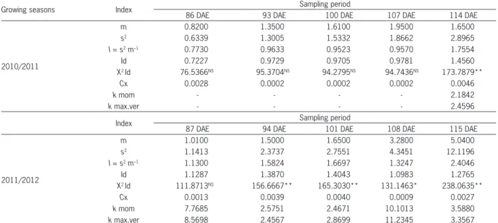
given level of infestation. When the average is equal to 0.75 nymph > 0.5 cm plus adults and when the aver-age is equal to 1.5 nymph > 0.5 cm plus adults of E. heros, the test probability of accepting H0 is 95 %, rec-ommending no control, and when the average is equal to 2.0 nymphs > 0.5 cm plus adults and when the aver-age is equal to 4.0 nymphs > 0.5 cm plus adults of E. heros, the probability of accepting H0 is 5 %, i.e., the probability of recommending control is 95 % (Figures 3 and 4). Thereafter, the expected number of samples E(N) was calculated. For the grain production fields, the maximum expected sample size was six sampling units, and for the seed production fields, nine sampling units (Figures 5 and 6), regardless of the size of the area, in homogeneous areas. If this criterion is not met, the area is divided into more homogeneous plots to facilitate the management of these areas.
Figure 1 – Decision lines of sequential sampling plan for the number of nymphs larger than 0.5 cm plus adults of Euschistus heros per sampling unit for grain production field of soybean. Jaboticabal – SP, Brazil, in the growing seasons 2010/2011 and 2011/2012.
0 5 10 15 20 25 30 35 40
1 2 3 4 5 6 7 8 9 10 11 12 13 14 15
Num
ber of
nym
phs
l
arger
than
0.
5
c
m
pl
us
adul
ts
by
s
am
pl
ing
uni
t
(A
c
c
um
ul
at
ed)
Number of sample units Continue sampling Accepted H1: m1= 4.0
S1= 4.4062 + 2.4852 N
Accepted H0: m0= 1.5 S0= -4.4062 + 2.4852 N Pest Control
No Pest Control
Figure 2 – Decision lines of sequential sampling plan for the number of nymphs larger than 0.5 cm plus adults of Euschistus heros per sampling unit for seed production fields of soybean. Jaboticabal – SP, Brazil in the growing seasons 2010/2011 and 2011/2012.
0 2 4 6 8 10 12 14 16 18 20
1 2 3 4 5 6 7 8 9 10 11 12 13 14 15
Num
ber of
nym
phs
l
arger
than
0.
5
c
m
pl
us
adul
ts
by
s
am
pl
ing
uni
t
(A
c
c
um
ul
at
ed)
Number of sample units Continue sampling Accepted H1: m1= 2.0
S1= 3.7112 + 1.2553 N
Accepted H0: m0= 0.75 S0= -3.7112 + 1.2553 N Pest control
No Pest control
Figure 3 – Characteristic operation curve OC(m) of the sampling plan for the average number of nymphs larger than 0.5 cm plus adults of Euschistus heros by the drop cloth technique for grain production fields of soybean. Jaboticabal – SP, Brazil, for the growing seasons 2010/2011 and 2011/2012.
0.00 0.10 0.20 0.30 0.40 0.50 0.60 0.70 0.80 0.90 1.00 1.10
0.00 1.00 2.00 3.00 4.00 5.00 6.00
Charac
teri
s
ti
c
operat
ion
c
urve
OC(m
)
Average number of nymphs larger than 0.5 cm plus adults by drop cloth technique
Figure 4 – Characteristic operation curve OC(m) of the sampling plan for the average number of nymphs larger than 0.5 cm plus adults of Euschistus heros by the drop cloth technique for seed production fields of soybean. Jaboticabal – SP, Brazil, for the growing seasons 2010/2011 and 2011/2012.
0.00 0.10 0.20 0.30 0.40 0.50 0.60 0.70 0.80 0.90 1.00 1.10
0.00 0.50 1.00 1.50 2.00 2.50 3.00 3.50 4.00
Charac
teri
st
ic
operat
ion
curve
OC(m
)
Average number of nymphs larger than 0.5 cm plus adults by drop cloth Technique
Figure 6 – Curve of the expected sample size E(N) in the sampling sequence for the average number nymphs larger than 0.5 cm plus adults of Euschistus heros by the drop cloth technique for seed production fields of soybean. Jaboticabal – SP, Brazil, for the growing seasons 2010/2011 and 2011/2012.
Table 4 – Sampling of nymphs > 0.5 cm plus adults of Euschistus heros for grain production fields of soybean. Jaboticabal – SP, Brazil.
Number of sampling units
Lower limit (S0) (No Pest
Control)
Number of nymphs > 0.5 cm
plus adults (Accumulated)
Superior Limit (S1) (Pest Control)
1 - 7
2 - 10
3 3 12
4 5 15
5 8 17
6 10 20
7 12 22
8 15 25
9 17 27
10 20 30
11 22 32
12 25 35
13 27 37
14 30 40
15 32 42
16 35 45
17 37 47
18 40 50
19 42 52
20 45 55
21 47 57
22 50 60
23 52 62
24 55 65
25 57 67
26 60 70
27 62 72
28 65 74
29 67 77
30 70 79
Table 5 – Sampling of nymphs > 0.5 cm plus adults of Euschistus heros for seed production fields of soybean. Jaboticabal – SP, Brazil.
Number of sampling units
Lower limit (S0) (No Pest
Control)
Number of nymphs > 0.5 cm
plus adults (Accumulated)
Superior Limit (S1) (Pest Control)
1 - 5
2 - 7
3 - 8
4 1 9
5 2 10
6 3 12
7 5 13
8 6 14
9 7 15
10 8 17
11 10 18
12 11 19
13 12 21
14 13 22
15 15 23
16 16 24
17 17 26
18 18 27
19 20 28
20 21 29
21 22 31
22 23 32
23 25 33
24 26 34
25 27 36
26 28 37
27 30 38
28 31 39
29 32 41
30 33 42
In conventional sampling, for 1-9 ha, six sam-pling points are required for decision making on the control of E. heros (Gallo et al., 2002). In this study, for grain production fields with average infestations of 1.5 nymph > 0.5 cm plus adults and 4.0 nymphs > 0.5 cm plus adults per drop cloth sampling, the ex-pected number of samplings were four and three, re-spectively, and for seed production fields with aver-age infestation of 0.75 nymphs > 0.5 cm plus adults and 2.0 nymphs > 0.5 cm plus adults per drop cloth sampling, the expected number of samplings being seven and five, respectively.
As regards the conventional sampling of cotton (Gossypium hirsutum L.) leafworm Alabama argillacea (Hübner, 1818) (Lepidoptera: Noctuidae), it is neces-sary to sample 100 cotton plants per hectare in order to make decisions about its control (Busoli et al., 2011). However, for sequential sampling, with an expected number of sampling units for an infestation of two lar-vae per plant, it is necessary to sample only 10 sam-0.00
1.00 2.00 3.00 4.00 5.00 6.00 7.00 8.00 9.00 10.00
0.00 0.50 1.00 1.50 2.00 2.50 3.00 3.50 4.00
Curve of
t
he ex
pec
ted
s
am
pl
e
s
ize E
(N)
pling units per hectare to make decisions (Fernandes et al., 2003).
The sequential sampling plan proposed in this study resulted in reducing the number of sampling units needed for decision-making for the control of E. heros, and, consequently, the time and costs required for a population survey of this species found on soybean.
Acknowledgements
To the Coordination for the Improvement of Higher Level Personnel (CAPES), for the Master’s scholarship of the first author and to the FCAV/UNESP for providing the infrastructure.
References
Allen, J.; Gonzales, D.; Gokhale, D.V. 1972. Sequential sampling
plans for the bollworms, Heliothis zea. Environmental
Entomology 1: 771-780.
Barbosa, J.C. 1992. The sequencial sampling = A amostragem sequencial. p. 205-211. In: Fernandes, O.A.; Correia, A.C.B.; Bortoli, S.A., eds. Integrated management of pests and nematodes = Manejo integrado de pragas e nematóides. FUNEP, Jaboticabal, SP, Brazil. (in Portuguese).
Bliss, C.I.; Owen, A.R.G. 1958. Negative binomial distribution
with a common K. Biometrika 45: 37-58.
Busoli, A.C.; Grigolli, J.F.J.; Fraga, D.F.; Souza, L.A.; Funichello, M.; Nais, J.; Silva, E.A. 2011. Current status of IPM practices for cotton in the Brazilian Cerrado = Atualidades no MIP algodão no Cerrado Brasileiro. p. 117-138. In: Busoli, A.C.; Fraga, D.F.; Santos, L.C.; Alencar, J.R.C.C.; Grigolli, J.F.J.; Janini, J.C.; Souza, L. A.; Viana, M.V.; Funichello, M., eds. Topics in agricultural entomology IV. Multipress, Jaboticabal, SP, Brazil. (in Portuguese).
Corrêa-Ferreira, B.S.; Azevedo, J. 2002. Soybean seed damage by different species of stink bugs. Agricultural and Forest Entomology 4: 145-150.
Costa, M.G.; Barbosa, J.C.; Yamamoto, P.T.; Leal, R.M.
2010. Spatial distribution of Diaphorina citri Kuwayama
(Hemiptera:Psyllidae) in citrus orchards. Scientia Agricola 67: 546-554.
Elliott, J.M. 1979. Some Methods for the Statistical Analysis of Samples of Benthic Invertebrates. Freshwater Biological Association, Ambleside, UK.
Fehr, W.R.; Caviness, C.E. 1977. Stages of Soybean Development. State University of Science and Techonoly, Ames, IO, USA. Fernandes, M.G.; Busoli, A.C.; Barbosa, J.C. 2003. Sequential
sampling of Alabama argillacea (Hübner) (Lepidoptera:
Noctuidae) on cotton crop. Neotropical Entomology 32: 117-122 (in Portuguese, with abstract in English).
Kogan, M.; Herzog, D.C. 1980. Sampling Methods in Soybean Entomology. Springer, New York, NY, USA.
Gallo, D.; Nakano, O.; Silveira Neto, S.; Carvalho, R.P.L.; Baptista, C.G.; Berti Filho, E.; Parra, J.R.P.; Zucchi, R.A.; Alves, S.B.; Vendramim, J.D.; Marchini, L.C; Lopes, J.R.S.; Omoto,
C. 2002. Agricultural Entomology = Entomologia Agrícola.
FEALQ, Piracicaba, SP, Brazil. (in Portuguese).
Green, R.H. 1966. Measurement of non-randomness in spatial distributions. Researches on Population Ecology 8: 1-7.
Hoffmann-Campo, C.B.; Moscardi, F.; Corrêa-Ferreira, B.S.; Oliveira, L.J.; Sosa-Gómez, D.R.; Panizzi, A.R.; Corso, I.C.; Gazzoni, D.L.; Oliveira, E.B. 2000. Pests of soybean in Brazil and its integrated management = Pragas da soja no Brasil e seu manejo integrado. EMBRAPA. Disponível em http://ag20. cnptia.embrapa.br/Repositorio/circtec30_000g46xpyyv02wx5o k0iuqaqkbbpq943.pdf
[Accessed Sept 25, 2013] (in Portuguese).
Morisita, M. 1962. Id-index, a measure of dispersion of individuals. Researches on Population Ecology 4: 1-7.
Panizzi, A.R.; Galileo, M.H.M.; Gastal, H.A.O.; Toledo, J.F.F.;
Wild, C.H. 1980. Dispersal of Nezara viridula and Piezodorus
guildinii nymphs in soybeans. Environmental Entomology 9:
293-297.
Rabinovich, J.E. 1980. Introducción a la Ecologia de Poblaciones Animales = Introdução à Ecologia de Populações de Animais. Editorial Continental, Ciudad de México, México (in Spanish). Sosa-Gómez, D.R.; Corso, I.C.; Morales, L. 2001. Insecticide
resistance to Endosulfan, Monocrotophos and Metamidophos
in the neotropical brown stink bug, Euschistus heros (F.).
Neotropical Entomology 30: 317-320.
Sosa-Gómez, D.R.; Silva, J.J.; Lopes, N.I.O.; Corso, I.C.; Almeida, A.M.R.; Moraes, G.C.P.; Baur, M.E. 2009. Insecticide
susceptibility of Euschistus heros (Heteroptera: Pentatomidae)
in Brazil. Journal of Economic Entomology 102: 1209-1216. Sosa-Gómez, D.R.; Silva, J.J. 2010. Neotropical brown stink bug
(Euschistus heros) resistance to Methamidophos in Paraná,
Brazil. Pesquisa Agropecuária Brasileira 45: 767-769.
Southwood, T.R.E. 1978. Ecological Methods. John Wiley, New York, NY, USA.
Taylor, L.R. 1961. Aggregation, variance and the mean. Nature 189: 732-735.
Wald, A. 1945. Sequential tests of statistical hypothesis. The Annals of Mathematical Statistics, 16: 117-186.