ABSTRACT: In this study, an accurate computational algorithm in the context of immersed boundary methods is developed and used to analyze an incompressible low around a pitching symmetric airfoil at Reynolds number (Re = 255). The boundary conditions are accurately implemented by an iterative procedure applied at each time step, and the pressure is also updated simultaneously. Flow phenomena, observed at different oscillation frequencies and amplitudes, are numerically modeled, and the physics behind the associated vortex dynamics is explained. It is shown that there are four low regimes associated with four wake structures. These include three symmetric low regimes, with adverse, favorable and no vortex effects, and an asymmetric low regime. The phenomena associated with these low regimes are discussed, and the critical or transitional values of the Strouhal (St) and normalized amplitude (AD) numbers are presented. It is shown that, at the ixed pitching amplitude, AD = 0.71, the transition from adverse (drag generation) to favorable (thrust generation) symmetric low regime occurs at St = 0.23. Moreover, at this particular amplitude, transition from symmetric to asymmetric regime occurs at St = 0.48. It is also shown that, at St = 0.22, the wake is always delected and the low is asymmetric for large enough amplitudes AD > 2. The dipole vortices and lift generation are two characteristics of asymmetric vortex street. This numerical study also reveals that the initial phase angle has a dominant effect on the appearance of dipole vortices and vortex sheet delection direction. Numerical results are in good agreement with the available experimental data.
KEYWORDS: Immersed boundary method, Flapping airfoil, Karman vortex street, Thrust generation, Lift generation.
Numerical Simulation of the Wake
Structure and Thrust/Lift Generation of a
Pitching Airfoil at Low Reynolds Number
Via an Immersed Boundary Method
Ali Akbar Hosseinjani1, Ali Ashraizadeh1
INTRODUCTION
Birds, insects and marine creatures use, and beneit from, the phenomena associated with lapping wings, tails and ins. Inspired by the nature, scientists and engineers have focused on the performance of oscillating wings and airfoils and have found that lapping mechanism is more eicient compared to the classical ixed wing designs at low Reynolds numbers (Re) (Davis 2007).
he low ield around a lapping airfoil is very complex due to the discontinuous production of vortices and transient interactions between them. Studies on pitching airfoils have shown that there are diferent low regimes associated with diferent wake patterns. For example, Kármán vortex street (KVS) and reverse Kármán vortex street (RKVS) are two diferent low patterns that result in drag enhancement and thrust generation, respectively. In addition, the vortices in the wake region of a pitching airfoil can be symmetric or delected, and this also afects the momentum exchange between the airfoil body and the surrounding luid (Ashraf 2010). It is, therefore, very important to understand the development of these low regimes, the transition from one regime to another and to quantify the favorable and adverse efects associated with lapping airfoils.
he transient low ield around lapping airfoils has been studied theoretically, experimentally and numerically for further understanding of the efects of parameters such as frequency,
1.Khajeh Nasir Toosi University of Technology – Faculty of Mechanical Engineering – Tehran – Iran.
Author for correspondence: Ali Akbar Hosseinjani | P.O.Box 19395 – 1999 – Tehran – Iran | Email: [email protected]
amplitude and lapping mode on the lit/thrust generation and momentum loss.
On the theoretical side, Jones et al. (1998) have used the efective angle of attack to explain the thrust generation by a lapping airfoil. he role of the vortex dynamics on thrust and drag generation, or momentum surfeit or deicit in the wake region, is explained by von Kármán and Burgers (1934). Also, Weis-Fogh (1973) explains how insects ly using the unsteady lit generation mechanism.
Many experimental studies have also been carried out. Anderson et al. (1998) have provided experimental results related to thrust generation through a combined pitching and plunging motion of a NACA0012 airfoil in a water tunnel. Based on this study, the optimum thrust is obtained at a Strouhal number (St) between 0.25 and 0.4. Taylor et al. (2003) have experimentally studied wing frequencies of 42 diferent birds, bats and insects and concluded that the Strouhal numbers associated with these natural lyers are between 0.19 and 0.41. hese results are in agreement with the results reported by Anderson
et al. (1998). Lentik et al. 2007 have experimentally studied the vortex dynamics of a lapping airfoil in a soap ilm tunnel at Re = 1,000 and reported that, at high amplitude oscillations, asymmetric wakes are generated when the frequency is increased. Godoy-Diana et al. (2008) have experimentally studied the vortex structure around a pitching airfoil and presented the results in the form of a parameter map for diferent wake types. Bohl and Koochesfahani (2009) have studied the wake patterns behind a sinusoidally pitching symmetric airfoil at various oscillation frequencies and concluded that the wake pattern can be controlled by adjusting the frequency, amplitude and the oscillation mode (shape of the oscillation wave form). hey have also reported the transition point at which the KVS regime turns to the RKVS one. Zanotti et al. (2014) studied, both experimentally and numerically, a pitching airfoil in deep dynamic stall condition. hey reported that, during upstroke motion, 3-D numerical models are in better agreement with the experiments as compared to 2-D models.
Considering the complexity of the vortex dynamics around a lapping airfoil and the continuous progress in computational algorithms and computer sotware and hardware, numerical simulation is becoming more and more popular. Wang (2000) has numerically calculated the low around a 2-D symmetric airfoil undergoing pure plunging motion by an incompressible Navier-Stokes solver at Re = 1,000 and reported that the low separates from both the leading and trailing edges at this
particular Re. Lewin and Haj-Hariri (2003), as well as Young and Lai (2007), have provided numerical results on wake structures and low regimes around plunging airfoils. According to the latter study, aerodynamic forces are more strongly afected by the leading edge vortices while the wake structure is mainly controlled by trailing edge vortices. Schnipper et al. (2009) have provided information regarding the efects of the wake pattern on aerodynamic forces for a lapping airfoil. He et al. (2012) have studied transition and symmetry-breaking in the wake of a lapping airfoil by an immersed boundary method (IBM). hey have presented results that show low patterns from the KVS regime to the RKVS one. Yu et al. (2012) investigated the asymmetric wake vortex structure around an oscillating airfoil both numerically and experimentally. hey reported that the delected wake appears around St = 0.31 for pitching amplitude equal to 5°. hey also reported that, as the St increases, the dipole mode of the vortex pair becomes more prevalent. Dipole vortex is necessary for the formation of asymmetric wake. Ren et al. (2013) reported that the direction of wake asymmetry changes at St = 0.37 for a ixed amplitude corresponding to α = 5°. Khalid
et al. (2014) have numerically simulated the equivalence of pitching and plunging motions found in a lapping NACA0012 airfoil. hey have reported that wake delection is observed, though not dominant, at low Strouhal numbers. Bai et al. (2014) used an immersed boundary method to simulate the turbulent low around a horizontal axis turbine operating under free surface waves. he IBM which is implemented in this investigation uses a 3-D inite volume solver. Also, Wei and Zheng (2014) have implemented an IBM to study the wake downstream of a 2-D heaving airfoil.
In this study, the physics behind the wake structure, the transition from one low regime to another and the thrust/lit performance of a sinusoidally lapping symmetric airfoil over a wide range of Strouhal numbers and oscillation amplitudes is studied. Furthermore, the efect of the initial phase angle on the delected vortex street, not suiciently discussed in the relevant literature, is studied. To carry out this investigation, an accurate computer code based on the IBM is developed and used to simulate the low. IBM is particularly well suited for moving boundary problems including the problem of low around a lapping airfoil.
force and pressure iteratively in an inner loop at each time step. Two test cases are used to validate the computational results.
he present numerical study is carried out at a constant Reynolds number (Re = 255). he airfoil is also selected such that the experimental results reported by Godoy-Diana et al. (2008) are numerically modeled. Furthermore, detailed information regarding the vortex shedding, time-averaged velocity ield, and aerodynamic coeicients at diferent oscillation frequencies and amplitudes is reported. he phenomenon of transition from drag-generating wake to thrust-generating wake is also discussed.
IMMERSED BOUNDARY METHOD
GEnERAl ViEWIn this section, some background information relevant to the commonly used IBMs is presented.
IBMs use a background uniform Cartesian grid, which does not generally conform to the boundary of the low domain. Boundary conditions are then imposed by source terms in the governing equations discretized on the background Cartesian mesh. In moving boundary problems, the displacement of boundary nodes corresponds to the shift of source terms between ixed grid points.
In IBMs, one has to distinguish between two diferent types of nodal points. Fixed Cartesian grid points are called the Eulerian points and the possibly moving boundary points are called the Lagrangian points. To numerically solve an incompressible low around a moving object via IBM, it is assumed that the boundary imposes force on the luid and the luid imposes an equal and opposite force on the boundary. In classical Peskin’s method, the immersed boundary is represented by a set of elastic ibers whose locations are tracked by Lagrangian points (Peskin 2002). Figure 1 shows the coordinates of Lagrangian and Eulerian points and the zone of inluence for the force term at Lagrangian point K.
he force terms on Lagrangian points, represented by F , are then related by the Hook’s law or a similar relation to the displacement of these points. hese force terms are distributed on Eulerian grid points by a proper delta-type function. herefore, boundary force at each Lagrangian point is distributed over a group of cells around that Lagrangian point. he forces exerted at the background grid points, f, are related to the boundary force as follows:
where:
x = (x, y) are the Cartesian coordinates of an Eulerian point; t is time; Γb is the boundary of the solid domain; s is the body-itted coordinate along the boundary; δ is a smooth Dirac delta function; X = (X, Y) are the Cartesian coordinates of a Lagrangian point.
k
Fk
Figure 1. (a) Lagrangian (X) and Eulerian (x) points; (b) zone
of inluence for the force term at Lagrangian point k (Lima e Silva et al. 2003).
he distributed forces on Eulerian points are used in the discrete governing equations as source terms. hese equations are then solved to calculate luid velocities at Eulerian grid points, represented by u. he velocities at boundary Lagrangian points, U, are calculated aterwards as follows:
where:
Ωs is the solid domain and Ωf is the luid domain. Note that discrete governing equations are solved at all Eulerian grid points regardless of the positions of those points. In other words, non-physical velocities are assigned to the Eulerian grid points outside of the low domain. hese numerical results are some by-products of the IBM computations.
The method just described is called the continuous forcing method and is often used to solve fluid-structure interaction problems with elastic boundary at low Reynolds numbers.
The direct forcing method, developed by Mohd-Yusof (1997) and further refined by Tseng and Ferziger (2003), Balaras (2004) and Mittal et al. (2008), is another approach in the family of immersed boundary techniques. his method is better suited for high Re lows. he force is implemented into the momentum equation directly by substituting the regularized no-slip condition near immersed boundary.
(1)
(2)
E x a c t i m p l e m e n t a t i o n o f t h e b o u n d a r y c o n d i t i o n s a s w e l l a s t h e s a t i s f a c t i o n o f c o n s e r v a t i o n l a w s a r e t w o m a j o r c o n c e r n s i n a l l I B M s . T o s a t i s f y m a s s a n d m o m e n t u m c o n s e r v a t i o n n e a r t h e b o u n d a r y , t h e c u t c e l l m e t h o d ( C h u n g 2 0 0 6 ) h a s a l s o b e e n d e v e l o p e d . I n t h i s m e t h o d , i n i t e v o l u m e s a r e d e i n e d s o t h a t i m m e r s e d b o u n d a r y c o i n c i d e s w i t h b o u n d a r y c e l l f a c e s . h i s m e t h o d a n d s o m e l a t e r i m p r o v e m e n t s , e.g. L s - S T A G ( C h e n y a n d B o t e l l a 2 0 1 0 ) , a r e r a t h e r m o r e c o m p l e x c o m p a r e d t o t h e t w o p r e v i o u s l y m e n t i o n e d m e t h o d s .
I n t h i s p a p e r , a n i t e r a t i v e - d i r e c t f o r c i n g I B M i s e m p l o y e d . V a r i a b l e s a t L a g r a n g i a n a n d E u l e r i a n g r i d p o i n t s a r e l i n ked through a simple discrete delta function. Details of the proposed method are given in the next section.
ThE PROPOSED COmPuTATiOnAl AlGORiThm Formulation and Force Term Calculations
In the formulation presented here, which has been proposed by Wang et al. (2008), a irst-order time discretization similar to Uhlmann’s method (Uhlmann 2005) is used to implement the Lagrangian force terms. he governing equations for incompressible low in the entire computational domain (Ωf + Ωg) are:
It is important to note that u is an intermediate velocity vector at Eulerian points that satisies the momentum equation without considering the efects of the boundary conditions. he superscript n indicates the last time step, and Δt is the time step. To calculate nodal velocity values that satisfy both the boundary conditions and governing equations, the efect of the force term should be added as follows:
where:
u is the velocity vector on the Eulerian points; P is the pressure; ρ is the luid density; ν is the kinematic viscosity, defined as ν = μ / ρ , where μ is the fluid dynamic viscosity; V
and V2 are the regular centered diference approximations for the gradient and Laplace operators, respectively. he source term f
in Eq. 3 is a fraction of the relevant external boundary force F
that acts at Eulerian grid point. he force term F is imposed at the Lagrangian point to enforce the desired velocity UΓ at the immersed boundary. his is done to assure that the velocities at Lagrangian points satisfy the no-slip boundary condition.
An estimate of the velocity can be obtained by the following equation:
Rewriting Eq. 7 at a Lagrangian point, it results in:
where:
Un+1 is the velocity at the Lagrangian point at time level
n + 1; U is an intermediate Lagrangian point velocity calculated as follows:
he velocity term Un+1 in Eq. 8 can now be replaced by
the known velocity at the boundary (UΓ ). his results in the following expression:
Force terms at Eulerian points can now be calculated using the discrete delta function:
where:
N is the number of Lagrangian points; ΔSk is the distance
between kth and (k – 1)th Lagrangian points.
Numerical Scheme
A inite diference method on a staggered grid is used in this study. he immersed boundary is discretized by N Lagrangian markers, Xk = (Xk, Yk), where the marker spacing is equal to
ΔS = Γb / N. he following discrete Dirac delta function is used to
transfer the information between Lagrangian and Eulerian points: (3)
(7)
(8)
(9)
(10)
(11)
(12) (4)
(5)
(6)
ˆ
where:
x and y are Cartesian coordinates at Eulerian point. he hat function, dh, which is equivalent to the quadratic interpolation scheme (Peskin 2002), is deined as follows:
where:
(u, û, u*)are Eulerian points.
Equation 22, with error tolerance ε = 0.001, is checked in each inner loop to impose the velocity boundary condition exactly. At the end of inner loop, the velocity and pressure are updated as follows:
where:
h is the grid size and r is a variable like (x - Xk) or (y - Yk) in Eq. 12.
To solve the Navier-Stokes equations, the fractional step method proposed by Kim and Moin (1985) is implemented. he non-linear convection term is treated by second-order Adams-Bashforth method, and Crank-Nicolson method is used for the discretization of the difusion terms. All the space derivatives are approximated by the second-order central diference method. The time advancement and calculation of flow field at time level n + 1 is carried out through the following steps. he irst u (intermediate velocity at Eulerian points) is calculated by Eq. 14.
hen, an inner loop is used to update pressure and impose velocity boundary condition in an iterative procedure. he following equations are used at the mth inner loop iteration:
Vector quantities, u, u* and u* , are the intermediate velocities between the time levels n and n + 1.
he computational algorithm can now be summarized as follows:
1. Obtain the intermediate velocity at grid points, u (x), by solving Eq. 14.
Start the inner loop:
2. Obtain the intermediate velocity at grid points, û (x), by solving Eq. 15.
3. Calculate the intermediate velocities at Lagrangian points, U (Xk) , using Eq. 16.
4. Obtain the force terms at Lagrangian points, Fn,m (X k),
by Eq. 17.
5. Distribute the Lagrangian forces among the Eulerian points using Eq. 18.
6. Correct the intermediate velocities and obtain u* (x) by Eq. 19.
7. Obtain u by Eq. 20.
8. Update pressure by solving Poisson equation — Eq. 21.
9. Check Eq. 22 for convergence; if the convergence is achieved, then go to step 10; otherwise, go to step 2. End of inner loop:
10. Update pressure and velocity by Eqs. 23 and 24.
11. Go to the next time step.
VALIDATION STUDIES
Two test cases are used to validate the proposed numerical method. he irst test case is a laminar low around a ixed circular cylinder which is steady at Re = 40 and unsteady at (13)
(21)
(22)
(23)
(24)
(14)
(15)
(16)
(17)
(18)
(19)
(20)
˜
˜ ˆ
˜
R e = 100. he calculated drag coeicients at various Reynolds numbers are compared to the values reported by Park et al. (1998) and Lima e Silva et al. (2003), shown in Table 1.
The second test case is a laminar flow around an inline (back and forth in the x direction) oscillating a circular cylinder in a stagnant fluid as described by Dütsch et al.
(1998). The periodic oscillation is given by the harmonic function, x = –Asin (2πfet) , in which A denotes the oscillation amplitude of the cylinder and fe is the frequency of the oscillation. Keulegan-Carpenter and Reynolds numbers are defined as KC = Um/fed and Re = Umd/ν, where, Um is the maximum velocity of cylinder during oscillation, d is the cylinder diameter and ν is the kinematic viscosity. The computation is performed at KC = 5 and Re = 100 at which the experimental and numerical results by Dütsch
et al. (1998) are available. Figure 4 shows the velocity profiles along the transverse (ya) axis at xa = –0.6d for two different phase positions compared to the experimental results of Dütsch et al. (1998). Velocity profiles (ua) agree relatively well with the experimental results.
Also, pressure and vorticity isolines have been compared with the numerical study of Guilmineau and Queutey (2002) in Figs. 5 and 6. Good agreement is evident.
Park et al. (1998) lima e Silva
et al. (2003) Present
method Re
2.78 2.81
2.79 10
2.01 2.04
2.02 20
1.51 1.54
1.52 40
1.35 1.40
1.37 80
1.33 1.39
1.35 100
Table 1. Comparison between the drag coeficients
computed by the present method and two reported results.
Also, the distributions of the pressure coefficient, CP = (P – P∞)/(1/2ρU∞), along the surface of circular cylinder at Re = 40 and Re = 100, are investigated. Here, U∞ is the far-ield free stream pressure which is assumed zero and is the free stream velocity. Figure 2 shows that the computational results in this study agree well with the results of Park et al. (1998). In the case of unsteady low (at Re = 100), pressure coeicients are averaged in time.
A comparison between the streamlines near the cylinder is shown in Fig. 3. In some of the conventional direct forcing methods, e.g. the method proposed by Su et al. (2007), the streamlines cross the boundary. his indicates that the boundary condition is not fully satisied. In the present method, iterative-direct forcing is employed, and the boundary conditions are fully satisied by updating the pressure and body force simultaneously in an iterative procedure.
Figure 2. Comparison of distribution of the pressure coeficient Cp along the cylinder surface for low past a stationary circular cylinder at Re = 40 and 100.
20
-1.5 -1 -0.5 0 0.5 1 1.5
60 100
θ [degrees] CP
140 180
Park et al. (1998)
Present method
Re = 40
Re = 100
Figure 3. Streamline around a circular cylinder. (a) Present
numerical method at Re = 40; (b) Conventional method (like Su et al. 2007) at Re = 40; (c) Present numerical method at Re = 100; (d) Conventional method (like Su et al. 2007) at Re = 100.
2
(a)
(b)
(c)
THE FLAPPING AIRFOIL MODEL
he computational domain and the lapping airfoil are shown in Fig. 7. he chord of the airfoil C is 23 mm and the diameter of the leading edge semi-circle D is 5 mm. hese dimensions
-1.5 -1 -0.5 0 0.5 1
-1 -0.5 0 0.5 1 1.5
ua
ya
-1.5 -1 -0.5 0 0.5 1
-1 -0.5 0 0.5 1 1.5
u a ya
Dütsch et al. (1998)
Present method
U
U
θ A
C = 23 mm
25C 15C
15C
5C
6C 18C
d
b a
c
D
=
5
mm
Figure 4. The x velocity component in the transverse (ya)
direction at xa = –0.6d for two different phase positions (φ = 2∏ft). (a) φ = 180°; (b) φ = 210°.
Figure 5. Vorticity isolines for two different phase positions
(φ = 2∏ft). (a) Guilmineau and Queutey 2002, at φ = 0°; (b) Present method, at φ = 0°; (c) Guilmineau and Queutey 2002, at φ = 95°; (d) Present method, at φ = 95°.
Figure 6. Pressure isolines for two different phase positions
(φ = 2∏ft). (a) Guilmineau and Queutey 2002, at φ = 0°; (b) Present method, at φ = 0°; (c) Guilmineau and Queutey 2002, at φ = 95°; (d) Present method, at φ = 95°.
U: far ield velocity.
Figure 7. Computational domain in this study.
(a)
(a)
(b)
(b)
(d)
(d)
(c)
(c)
(a)
(b)
(25) are chosen to simulate the experimental study carried out by Godoy-Diana et al. (2008).
In Eq. 25, θ
0 is the initial angle of attack and θ A is the
maximum angle of attack associated with the amplitude AD, as shown in Fig. 7. A 1,200 x 720 uniform grid is used as the background Cartesian mesh, and the Δt depends on the oscillation frequency. The time step is chosen so that each cycle of the oscillation corresponds to 2,000 time steps. For example, when the Strouhal number is St = 0.22, the time step is Δt = 1.14 x 10⁻⁴ s. Relevant flow parameters are taken from
the experiment of Godoy-Diana et al. (2008), i.e. Re = 255,
U∞ = 0.1 m/s, and ρ = 1 kg/m3. The viscosity is tuned in each
numerical test so that Re = 255 is kept fixed in all cases. A grid reinement study was carried out at AD = 0.71 and St = 0.22. he results are shown in Table 2 for 4 grid sizes. In Table 2, C is the chord of the airfoil and CD is the drag coeicient computed as follows:
Grid size Grid resolution CD
0.0625C 400 x 240 0.781
0.0416C 600 x 360 0.762
0.03125C 800 x 480 0.752
0.025C 1,000 x 600 0.748
0.02083C 1,200 x 720 0.745
0.0166C 1,500 x 900 0.745
Table 2. Grid reinement study for drag coeficient.
h
L∞
L∞ L2
y direction velocity component
x direction velocity component
h2
h2
h
h
10-1
10-2
10-3
10-3 10-2
10-2
10-1
10-1
100
10-4
10-5
10-3
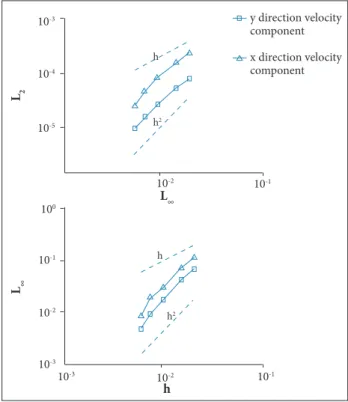
Figure 8. Grid convergence study. (a) L2 norm; (b) X norm.
SIMULATION RESULTS
Before presenting the computational results, it is appropriate to briely discuss some phenomena associated with lapping airfoils. As explained next, these phenomena are simulated and observed in this numerical study and have also been reported by Yu et al. (2012) and Ren et al. (2013).
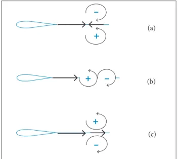
An airfoil lapping in a luid generates two main vortices near the leading edge. Deining the positive vortex as a counter clockwise vortex, as shown in Fig. 9, a negative vortex is generated at the upper surface of the foil and a positive vortex is generated at its lower surface. he strengths of these leading edge vortices and their subsequent positions behind the foil depend on the lapping amplitude and frequency for a given Re. When these vortices shed away from the airfoil, they alter the low pattern in the wake region. hree diferent scenarios regarding the orientation of the vortex pair in the wake region are shown in Fig. 9. For low values of oscillation frequency/ amplitude, the upper (negative) and lower (positive) vortices keep their initial relative positions with respect to the symmetry line of the airfoil. In this mode of lapping motion, the momentum of the flow in the wake region is reduced due to the adverse efect of vortex system on the main low (Fig. 9a). At higher In Eq. 26,
(
F (Xk))
x terms are the x-components of the forcesat Lagrangian points.
All results presented in this paper are obtained using the 1,200 x 720 grid. Figure 8 shows the grid convergence study. he results for the inest grid are considered accurate, and the
L2 and L∞ norms of the error obtained on the coarser grids are calculated and shown in Fig. 8. he results demonstrate the second-order accuracy of the method. he norms L2 and L∞ are deined as follows:
where:
+
+
+
–
–
–
frequencies/amplitudes, the vortex pair rolls into the wake region in an aligned situation shown in Fig. 9b. At still higher frequency/amplitude, the leading edge vortices cross the symmetry line behind the foil. In other words, the negative vortex appears below the symmetry line and the positive one appears above that line in this case (Fig. 9c). he low symmetry breaks down at more intensiied lapping, and a diverted jet of energized low is observed.
he vortex pair shown in Fig. 9a, results in momentum loss, and the low pattern is known as the Kármán (or Benard-von Kármán) vortex street. hese vortices are clearly drag generating vortices. In contrast, the vortex pair shown in Fig. 9c enhances the wake low momentum, and the pattern is known as the reverse Kármán vortex street. he RKVS is, therefore, a thrust-generating vortex street. When the two vortices are aligned, as shown in Fig. 9b, they have no favorable or adverse efect on the main low, shown by the thick black arrow.
he asymmetric or delected jet low regime is a thrust and lit-producing regime and is here called the asymmetric reverse Kármán vortex street regime (ARKVS) for the sake of briefness. In other words, in addition to the thrust production, side force is also generated due to the asymmetric nature of the low in the ARKVS regime.
If the lapping airfoil is used as a propulsive device, it is obviously necessary to realize how and when the low regime
Figure 9. (a) Kármán vortex street (drag-generating
vortex); (b) Aligned vortex; (c) Reverse Kármán vortex street (thrust-generating vortex). The black arrow shows the main low direction and the gray one shows the low direction generated by vortices.
changes. For a speciied Re, a performance map can be developed for both analysis and design purposes.
In this paper, two groups of numerical studies are carried out and reported to quantitatively investigate the phenomena just described. First, the St is ixed, and the efects of oscillation amplitude are considered. hen, the oscillation amplitude is ixed, and the efects of the frequency variation or St are studied. Finally, a map which shows the efects of the variation of both frequency and amplitude is presented.
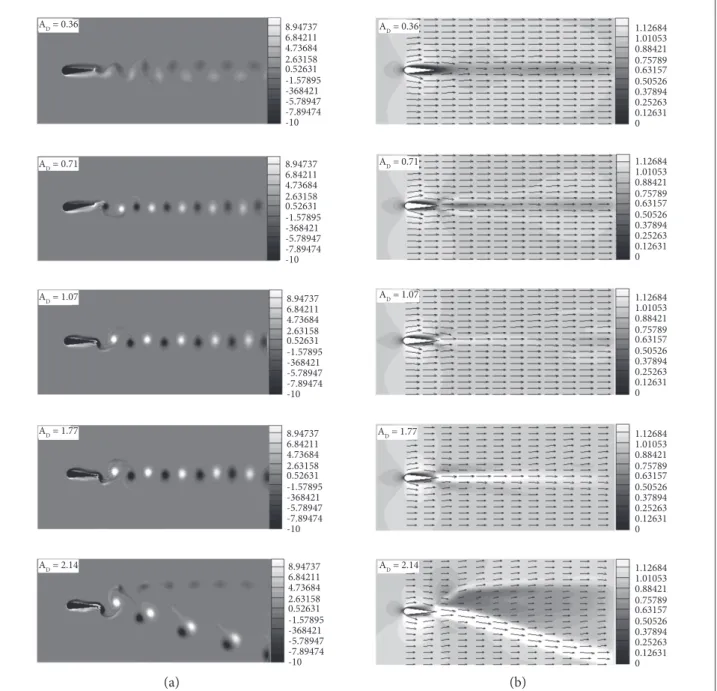
FlAPPinG AT FixED FREquEnCY (St = 0.22) Vortex structures and calculated average luid velocities at grid points are shown in Fig. 10 for St = 0.22, as well as AD = 0.36; 0.71; 1.07; 1.77 and 2.14. he calculated velocities are average values in an oscillation cycle, and the contour of the velocity ield is also shown in each case for further clariication. As Fig. 10 shows two main leading edge vortices formed and shed away from the airfoil as a result of the lapping motion. It is clearly seen that boundary layer separation from the top and bottom sides of the lapping airfoil alters the pattern of the vortex street. At AD = 0.36, momentum loss in the wake region is observed in the corresponding velocity-time averaged contour diagram. his is a drag generating KVS low regime. By increasing the amplitude, negative and positive vortices are positioned along the symmetry line behind the airfoil at AD = 0.71. In this aligned vortex regime, some loss in luid momentum exists due to viscous efects. However, the vortex system does not play a signiicant role in momentum transfer downstream. Based on the numerical results, transition from the KVS to RKVS regime occurs at AD ~ 0.72. Further increase in the lapping amplitude, represented by AD = 1.07 and AD = 1.77, results in the intensiication of the symmetric jet low and the propulsive force. his intensiication of the momentum transfer is clearly seen in the corresponding velocity-time averaged contour diagrams. At a higher lapping amplitude, i.e. AD = 2.14, the symmetry in the low ield breaks down, and the asymmetric low regime is observed. his corresponds to the ARKVS regime in which reactive side forces are generated.
The physics behind the asymmetric flow regime is not understood quite well, but the phenomenon may possibly be attributed to the intensive interactions between leading and trailing edge vortices (Yu et al. 2012). It is known that in the ARKVS regime a strong dipole vortex is formed on one side of the symmetry line, and a weaker single vortex is shed on the other side. Dipole vortex is made up of two vortices with diferent signs that are shed in each pitching cycle. In this vortex (a)
(b)
structure, corresponding to AD = 2.14, the jet-like low is bent towards the side of the strong dipole vortex as shown in Fig. 10.
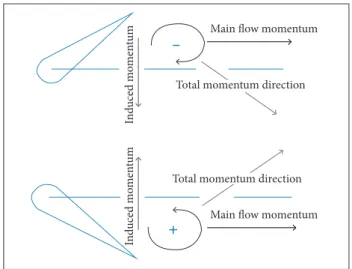
he schematics in Fig. 11 help to better understand why the KVS low regime changes to the RKVS regime. At low oscillation amplitudes, the induced momentum generated by airfoil pitching motion is not strong enough to push the vortex generated at one side of the foil to move to the other side. By increasing the oscillation amplitude, the push becomes strong enough to switch the positions of negative and positive vortices and to convert the KVS regime to the thrust-producing RKVS regime.
8.94737 6.84211 4.73684 2.63158 0.52631 -1.57895 -368421 -5.78947 -7.89474 -10
1.12684 1.01053 0.88421 0.75789 0.63157 0.50526 0.37894 0.25263 0.12631 0
1.12684 1.01053 0.88421 0.75789 0.63157 0.50526 0.37894 0.25263 0.12631 0
1.12684 1.01053 0.88421 0.75789 0.63157 0.50526 0.37894 0.25263 0.12631 0
1.12684 1.01053 0.88421 0.75789 0.63157 0.50526 0.37894 0.25263 0.12631 0
1.12684 1.01053 0.88421 0.75789 0.63157 0.50526 0.37894 0.25263 0.12631 0 8.94737
6.84211 4.73684 2.63158 0.52631 -1.57895 -368421 -5.78947 -7.89474 -10
8.94737 6.84211 4.73684 2.63158 0.52631 -1.57895 -368421 -5.78947 -7.89474 -10
8.94737 6.84211 4.73684 2.63158 0.52631 -1.57895 -368421 -5.78947 -7.89474 -10
8.94737 6.84211 4.73684 2.63158 0.52631 -1.57895 -368421 -5.78947 -7.89474 -10 AD = 0.36
AD = 0.71
AD = 1.07
AD = 1.77
A
D = 2.14 AD = 2.14
A
D = 0.36
A
D = 0.71
A
D = 1.07
A
D = 1.77
Figure 10. (a) Vortex shedding and (b) Time-averaged velocity at St = 0.22 and AD = 0.36; 0.71; 1.07; 1.77 and 2.14.
To further investigate and quantify the intensiied jet low behind the foil, time averaged horizontal velocities along a-b
and c-d lines, shown in Fig. 7, are calculated and shown in Figs. 12 and 13, respectively. It is seen that the velocity behind the airfoil at AD = 0.36 is decreased due to the drag generating KVS regime. At AD = 0.71, no net momentum is transferred to the main low by the aligned vortex system. However, viscous efects reduce the velocity behind the airfoil slightly. At AD = 1.07 and 1.77, velocity and momentum behind the airfoil increase due to the thrust-generating RKVS regime. Figure 9 makes it
c l e ar that there is a jet-like low at the middle of c-d line. his
corresponds to the transition from KVS to RKVS.
Simulation results also provide detailed information regarding the transition from symmetric RKVS to ARKVS low regime. By considering the results shown in Fig. 14, it is concluded that the transition occurs at normalized amplitude very close to AD = 2 for this particular lapping airfoil.
At AD = 2, the dipole vortex is not recognizable but the delection of the vortex sheet has just been initiated. At higher AD values, the jet delection and dipole vortex structure are clearly seen.
he calculated transient lit coeicients corresponding to AD = 0.71; 1.77 and 2.14 are shown in Fig. 15. Here, the lit coeicient is calculated as follows:
Main flow momentum
Main flow momentum Total momentum direction
Total momentum direction
In
d
uce
d m
o
m
en
tum
In
d
uce
d m
o
m
en
tum
–
+
0 0.4 0.8 1.2 1.6
a 2 4 6 8 1 0 b
X/C
u
/
U
1 2 1 4 1 6 1 8
AD = 0.36
A D = 0.71 A
D = 1.07 AD = 1.77
Figure 11. (a) The induced momentum pushes the
negative vortex at the upper surface downwards; (b) The induced momentum pushes the positive vortex at the lower surface upwards.
u: velocity behind the airfoil; x: distance behind the airfoil.
Figure 12. Time averaged horizontal velocity along a-b line,
shown in Fig. 7, at St = 0.22 and 4 different amplitudes. A non-dimensional coordinate along a-b line is employed.
AD = 0.36 A
D = 0.71 A
D = 1.07 AD = 1.77
0.9 1.1 1.3 1.5
u
/
U
0
c 1 2 3 d
X/C
4 5 6
A
D = 2
A D = 2.04
A D = 2.08
8.94737 6.84211 4.73684 2.63158 0.52631 -1.57895 -368421 -5.78947 -7.89474 -10
8.94737 6.84211 4.73684 2.63158 0.52631 -1.57895 -368421 -5.78947 -7.89474 -10
8.94737 6.84211 4.73684 2.63158 0.52631 -1.57895 -368421 -5.78947 -7.89474 -10
Figure 13. Time averaged horizontal velocity along c-d line,
shown in Fig. 7, at St = 0.22 and 4 different amplitudes. A non-dimensional coordinate along c-d line is employed.
Figure 14. Asymmetric KVS at (a) AD = 2, (b) 2.04 and (c) 2.08.
(a)
(b)
(c) (29)
where:
(
F (Xk))
y values are the y-components of the force at boundaryA
D = 0.71 and 1.77 are symmetric with respect to the CL = 0
line, meaning that no side (lit) force is generated at these amplitudes. In contrast, the CL curve corresponding to AD = 2.14 is not symmetric with respect to the CL = 0 line, which means that there is a net side force (lit) in this case. he average lit coeicients at various lapping amplitudes and St = 0.22 are shown in Fig. 16. It is clearly seen that lit generation starts close to AD = 2. As shown in this igure, when the delected vortex is generated behind the airfoil, a side force (lift) is produced. Therefore, the side force is an indication of the formation of a delected vortex behind the airfoil.
To understand what exactly happens near the transition point, which results in transition from symmetric to delected vortex, the vortex patterns are investigated at 4 time steps, t = 2T; t = 4T; t = 6T and t = 8T, being T the period of oscillation. As shown in Fig. 17, the first dipole vortex separates from the trailing edge at t = 2T. his dipole vortex is strong enough to bend the low direction. Ater that, second and third dipole vortices separate from the trailing edge and follow the irst dipole vortex. hese dipole vortices are then
Figure 16. The effect of oscillation amplitude on average lift
coeficient for St = 0.22.
Figure 15. Transient lift coeficient for St = 0.22 and AD =
0.71, 1.77 and 2.14.
A ve ra g e CL A D
K VS zone RKVS zone
De fl ected vortex zone
A lig n e d v o r t e z zo n e 0 0 4 8 12 16
1 2 3
0.7 0.72 8.94737 6.84211 4.73684 2.63158 0.52631 -1.57895 -368421 -5.78947 -7.89474 -10 8.94737 6.84211 4.73684 2.63158 0.52631 -1.57895 -368421 -5.78947 -7.89474 -10 8.94737 6.84211 4.73684 2.63158 0.52631 -1.57895 -368421 -5.78947 -7.89474 -10 8.94737 6.84211 4.73684 2.63158 0.52631 -1.57895 -368421 -5.78947 -7.89474 -10 A
D = 2.14 t = 8T AD = 2.14
t = 6T AD = 2.14
t = 4T AD = 2.14
t = 2T
8.94737 6.84211 4.73684 2.63158 0.52631 -1.57895 -368421 -5.78947 -7.89474 -10 8.94737 6.84211 4.73684 2.63158 0.52631 -1.57895 -368421 -5.78947 -7.89474 -10
AD = 2.14 A
D = 2.14
AD = 0.71
AD = 1.77
AD = 2.14
-100 0 50 100
CL
14 16 18 20 22 24 26
Time [s]
stretched along the vortex street and result in symmetry breaking. It is clear that the irst dipole vortex is very important in the sense that it determines the delected vortex direction. Numerical analysis shows that, when initial phase angle alters, the delected vortex direction alters too. his is clearly seen in Fig. 18.
Figure 17. Asymmetric KVS at (a) t = 2T, (b) 4T, (c) 6T and (d) 8T.
Figure 18. Shedding vortices at 2 initial phase angles with
90° difference. (a) Initial phase = 0°; (b) Initial phase = 90°.
no. Type of vortex Effect on the low Range of oscillation amplitude
1 K V S
( d r ag generating vortex)
Decreasing momentum behind the airfoil/
increasing the drag force AD < 0.70
2 Aligned vortex street (neutral type vortex)
Neither decreasing nor increasing
momentum behind the airfoil 0.70 < AD < 0.72
3 (thrust generating vortex)RKVS
Increasing momentum behind the airfoil/ decreasing the drag force and then
generating a thrust force
0.72 < AD < 2
4 (thrust/lit generating vortex)Delected vortex Simultaneous thrust and lit force generation 2 < AD
Table 3. Vortex types and low ield effects for various AD values at St = 0.22.
Table 3 summarizes the vortex types and low ield efects for various AD values at St = 0.22.
FlAPPinG AT FixED AmPliTuDE (AD = 0.71)
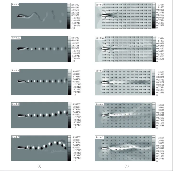
The effect of St on the vortex structure and thrust performance is now studied for ixed oscillation amplitude AD = 0.71 and diferent values of St: 0.1; 0.22; 0.3; 0.4 and 0.5. Vortex shedding and average velocity contours in this case are shown in Fig. 19.
Once again, to further explore the flow features, average horizontal velocities on a-b and c-d lines are calculated and shown in Figs. 20 and 21, respectively. The same trends explained before regarding Figs. 12 and 13 are observed here again.
Figure 22 shows the time history of lift coefficient for three different Strouhal numbers, i.e. St = 0.22; 0.3 and 0.5, and Fig. 23 shows the effect of the St on average lift coefficient for AD = 0.71. The same trends explained before regarding Figs. 15 and 16 are observed here again. It is clear that lift is generated for St > 0.48 in this case.
Table 4 summarizes the vortex types and low ield efects for various St values at AD = 0.71.
no. Type of vortex Effect on the low Range of Strouhal number
1 KVS
(drag generating vortex)
Decreasing momentum behind the airfoil/
increasing the drag force St < 0.22
2 Aligned vortex street (neutral type vortex)
Neither decreasing nor increasing
momentum behind the airfoil 0.21 < St < 0.23
3 RKVS
(thrust generating vortex)
Increasing momentum behind the airfoil/ decreasing the drag force and then
generating a thrust force
0.23 < St < 0.48
4 Delected vortex
(thrust/lit generating vortex)
Simultaneous thrust and lit force
generation 0.48 < St
Table 4. Vortex types and low ield effects for various St values at AD = 0.22.
PERFORmAnCE mAP FOR A RAnGE OF St nORmAlizED AmPliTuDE
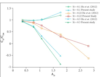
The effects of both amplitude and frequency on the drag/ thrust coefficient are shown in Fig. 24 and compared to the results reported by He et al. (2012). The drag coefficient for the corresponding motionless airfoil is CD0 = 0.86. As mentioned before, in the RKVS regime, the vortex system transfers momentum to the flow and generates thrust force. The situation CD = 0 in Fig. 24 corresponds to a situation in which the RKVS regime generates just enough thrust to overcome the drag. The reduction of drag coefficient for high values of amplitude/frequency corresponds to more thrust generation in the RKVS regime.
in Fig. 25 represent different types of vortex systems and flow regimes described previously.
The KVS regime, which is characterized by zone number 1 in Fig. 25, is observed when at least one of AD or St values is sufficiently low. The lower-left zone of the map corresponds to the KVS. At moderately low AD and St values, characterized by zone number 2, the aligned vortex system is developed. This corresponds to a flow regime between KVS and RKVS. Zone 3 in Fig. 25 represents the RKVS regime. As shown in
Fig. 25, the RKVS is formed at the middle of the map. Note that the zero drag (CD = 0) line lies in this region of the map as well. At the left-hand side of the CD = 0 line in zone 3, the generated thrust is still less than the drag. Propulsive force is obtained at oscillations corresponding to the right-hand side of the CD = 0 line in zone 3. Finally, the thrust and lift generating regime, i.e. the ARKVS regime, is represented by zone 4 in Fig. 25. This regime is obtained when both frequency and amplitude are sufficiently high.
1.13684 1.01053 0.88421 0.75789 0.63157 0.50526 0.37894 0.25263 0.12631 0 8.94737
6.84211 4.73684 2.63158 0.52631 -1.57895 -3.68421 -5.78947 -7.89474 -10
8.94737 6.84211 4.73684 2.63158 0.52631 -1.57895 -3.68421 -5.78947 -7.89474 -10
8.94737 6.84211 4.73684 2.63158 0.52631 -1.57895 -3.68421 -5.78947 -7.89474 -10
8.94737 6.84211 4.73684 2.63158 0.52631 -1.57895 -3.68421 -5.78947 -7.89474 -10
8.94737 6.84211 4.73684 2.63158 0.52631 -1.57895 -3.68421 -5.78947 -7.89474 -10
1.13684 1.01053 0.88421 0.75789 0.63157 0.50526 0.37894 0.25263 0.12631 0
1.13684 1.01053 0.88421 0.75789 0.63157 0.50526 0.37894 0.25263 0.12631 0
1.42105 1.26316 1.10526 0.94736 0.78947 0.63157 0.47368 0.31578 0.15789 0
1.42105 1.26316 1.10526 0.94736 0.78947 0.63157 0.47368 0.31578 0.15789 0 St = 0.5
St = 0.4
St = 0.3
St = 0.22
St = 0.1
St = 0.5
St = 0.4
St = 0.3
St = 0.22
St = 0.1
Figure 19. (a) Vortex shedding; (b) Time-averaged velocity at AD = 0.71, and St = 0.1; 0.22; 0.3; 0.4 and 0.5.
Figure 21. Average horizontal velocities at grid points along c-d line at AD = 0.71 and St = 0.1; 0.22; 0.3 and 0.4. A non-dimensional coordinate along c-d line is employed.
Figure 20. Average horizontal velocities at grid points along
a-b line at AD = 0.71 and St = 0.1; 0.22; 0.3 and 0.4. A non-dimensional coordinate along a-b line is employed.
Figure 24. Drag coeficients in terms of the normalized
amplitude at St = 0.1; 0.22 and 0.3.
Figure 23. The effect of St on average lift coeficient for
AD = 0.71.
Figure 22. Transient lift coeficient for AD = 0.71 and
St = 0.22; 0.3 and 0.5.
St = 0.1 St = 0.22 St = 0.3 St = 0.4
0.8 1 1.2 1.4 1.6 1.8 2
u/U
0
c 1 2 X/C3 4 5 6d
0 0 .5
0 1 1.5 2 2.5
a b
2 4 6 8 10
X/C
u/U
12 14 16 18
St = 0.1 St = 0.22 St = 0.3 St = 0.4
X: 22.98 Y: -258.6
X: 24.96 Y: -79
X: 25.9 Y: 79 X: 23.46
Y: 252.5
St = 0.22 St = 0.3 St = 0.5
-250 -150 -5 50 150 250
CL
14 23 24 25 26 27 28 29 30
Time [s]
C
L
St
K VS zone RKVS zone
De fl e cted vortex zone
A
lig
n
ed v
o
rt
e
z zo
n
e
0.1 0.3 0.5 0.7
1 3 5 7
0.23
0.21 0.48
St = 0.1 He et at. (2012)
St = 0.1 Present stu d y
St = 0.22 He et at. (2012)
St = 0.22 Present Study
St = 0.3 He et at. (2012)
St = 0.3 Present study
0 -1
-0.5 0 0.5 1 1.5
0.5 1 1.5
A D
CD
/C
D
0
2 2.5 3
Figure 25. A lapping foil performance map. Zone 1: Kármán
vortex street; zone 2: aligned vortex street; zone 3: reverse Kármán vortex street; zone 4: asymmetric reverse Kármán vortex street.
+ +
+ + + + + + + +
++ + +
+ + + +
+ +
+
CD = 0 4
3 2
1 3
2
1
0
0.1 0.2 0.3 0.4 0.5
St
CONCLUSIONS
In th is paper, an IBM is employed to simulate the low around a
lapping airfoil. he boundary conditions are accurately implemented by an iterative procedure applied at each time step. Vortex and wake patterns as well as lit and drag coeicients are studied at diferent oscillation amplitudes and frequencies. Four distinguished low regimes, controlled by the vortex system generated due to the lapping motion, are observed. hese low regimes are the KVS, the Aligned Vortex Street (AVS), the RKVS and inally the ARKVS. he KVS regime generates drag; the AVS is a neutral regime with no net momentum transfer to the main low; the RKVS is a thrust producing regime; and the ARKVS is a thrust and lit generating low regime. For the particular symmetric airfoil used in this study, two groups of lapping scenarios are studied at a ixed Reynolds
number (Re = 255). First, the frequency is ixed at St = 0.22, and the amplitude is changed. hen the amplitude is ixed at AD = 0.71, and the oscillation frequency is altered. For the ixed frequency case, St = 0.22, the transition from KVS to RKVS occurs at AD = 0.72, and the ARKVS is developed around AD = 2. For the fixed amplitude oscillation, AD = 0.71, the transition from KVS to RKVS occurs at St = 0.23, and the ARKVS is developed around St = 0.48. Vorticity and velocity contours are presented, which helps to understand the physics behind the low. he efects of the dipole vortex system in delecting the wake low are also discussed. he computational results compared to the available experimental data show that the iterative-direct forcing immersed boundary method is a reliable tool for studying complex transient lows such as the low around a lapping airfoil.
REFERENCES
Anderson JM, Streitlien K, Barrett DS, Triantafyllou MS (1998) Oscillating foils of high propulsive eficiency. J Fluid Mech 360:41-72. doi: 10.1017/S0022112097008392
Ashraf MA (2010) Numerical simulation of the low over lapping airfoils in propulsion and power extraction regimes (PhD thesis). Australia: School of Engineering and Information Technology.
Bai X, Avital EJ, Munjiza A, Williams JJR (2014) Numerical simulation of a marine current turbine in free surface low. Renew Energ 63:715-723. doi: 10.1016/j.renene.2013.09.042
Balaras E (2004) Modeling complex boundaries using an external force ield on ixed cartesian grids in large eddy simulations. Comput Fluids 33(3):375-404. doi: 10.1016/S0045-7930(03)00058-6
Bohl DG, Koochesfahani MM (2009) MTV measurements of the vertical ield in the wake of an airfoil oscillating at high reduced frequency. J Fluid Mech 620:63-88. doi: http://dx.doi.org/10.1017/ S0022112008004734
Cheny Y, Botella O (2010) The LS-STAG method: a new immersed boundary/level-set method for the computation of incompressible viscous lows in complex moving geometries with good conservation properties. J Comput Phys 229(4):1043-1076. doi: 10.1016/ j.jcp.2009.10.007
Chung MH (2006) Cartesian cut cell approach for simulating incompressible lows with rigid bodies of arbitrary shape. Comput Fluids 35(6):607-623. doi: 10.1016/j.compluid.2005.04.005
Davis WA (2007) Nano air vehicle: a technology forecast. Technical Report. Montgomery (AL): Blue Horizons Paper, Center for Strategy and Technology, Air War College.
Dütsch H, Durst F, Becker S, Lienhart H (1998) Low-Reynolds-number low around an oscillating circular cylinder at low Keulegan-Carpenter numbers. J Fluid Mech 360:249-264. doi: 10.1017/ S002211209800860X
Godoy-Diana R, Aider JL, Wesfreid JE (2008) Transitions in the
wake of a lapping foil. Phys Rev E 77:207-221. doi: 10.1103/ PhysRevE.77.016308
Guilmineau E, Queutey P (2002) A numerical simulation of vortex shedding from an oscillating circular cylinder. J Fluid Struct 16(6):773-794. doi: 10.1006/jls.2002.0449
He GY, Wang Q, Zhang X, Zhang SG (2012) Numerical analysis on transitions and symmetry-breaking in the wake of a lapping foil. Acta Mech Sinica 28(6):1551-1556. doi: 10.1007/s10409-012-0158-8
Jones KD, Dohring CM, Platzer MF (1998) Experimental and computational investigation of the Knoller-Betz effect. AIAA Journal 36(7):1240-1246. doi: 10.2514/2.505
Khalid MSU, Akhtar I, Durrani NI (2014) Analysis of Strouhal number based equivalence of pitching and plunging airfoils and wake delection. J Aerospace Eng 229(8). doi: 10.1177/0954410014551847
Kim J, Moin P (1985) Application of a fractional-step method to incompressible Navier-Stokes equations. J Comput Phys 59(2):308-323. doi: 10.1016/0021-9991(85)90148-2
Lewin GC, Haj-Hariri H (2003) Modeling thrust generation of a two dimensional heaving airfoil in a viscous low. J Fluid Mech 492:339-362. doi: 10.1017/S0022112003005743
Lima e Silva ALF, Silveira-Neto A, Damasceno JJR (2003) Numerical simulation of two-dimensional lows over a circular cylinder using the immersed boundary method. J Comput Phys 189(2):351-370. doi: 10.1016/S0021-9991(03)00214-6
Mittal R, Dong H, Bozkurttas M, Najjar FM, Vargas A, Von Loebbecke A (2008) A versatile sharp interface immersed boundary method for incompressible lows with complex boundaries. J Comput Phys 227(10):4825-4852. doi: 10.1016/j.jcp.2008.01.028
Park J, Kwon K, Choi H (1998) Numerical solutions of flow past a circular cylinder at Reynolds numbers up to 160. J Mech Sci Technol 12(6):1200-1205. doi: 10.1007/BF02942594
Peskin C (2002) The immersed boundary method. Acta Numer 11:479-517. doi: 10.1017/S0962492902000077
Ren W, Hu H, Liu H, Wu JC (2013) An experimental investigation on the asymmetric wake formation of an oscillating airfoil. Proceedings of the 51st AIAA Aerospace Sciences Meeting including the New Horizons Forum and Aerospace Exposition, Paper. 0794; Grapevine, USA.
Schnipper T, Andersen A, Bohr T (2009) Vortex wakes of a lapping foil. J Fluid Mech 633:411-423. doi: 10.1017/S0022112009007964
Su SW, Lai MC, Lin CA (2007) An immersed boundary technique for simulating complex lows with rigid boundary. Comput Fluids 36(2):313-324. doi: 10.1016/j.compluid.2005.09.004
Taylor GK, Nudds RL, Thomas ALR (2003) Flying and swimming animals cruise at a Strouhal number tuned for high power eficiency. Nature 425:707-711. doi: 10.1038/nature02000
Tseng YH, Ferziger JH (2003) A ghost-cell immersed boundary method for low in complex geometry. J Comput Phys 192(2):593-623. doi: 10.1016/j.jcp.2003.07.024
Uhlmann M (2005) An immersed boundary method with direct forcing for the simulation of particulate lows. J Comput Phys 209(2):448-476. doi: 10.1016/j.jcp.2005.03.017
Von Kármán T, Burgers MJ (1934) Aerodynamic theory. Vol. 2. Berlin: Springer.
Wang Z, Fan J, Luo K (2008) Combined multi-direct forcing and immersed boundary method for simulating lows with moving particles. Int J Multiphas Flow 34(3):283-302. doi: 10.1016/ j.ijmultiphaselow.2007.10.004
Wang ZJ (2000) Vortex shedding and frequency selection in lapping light. J Fluid Mech 410:323-341. doi: 10.1017/ S0022112099008071
Wei Z, Zheng ZC (2014) Mechanisms of wake delection angle change behind a heaving airfoil. J Fluid Struct 481-13. doi: 10.1016/ j.jluidstructs.2014.02.010
Weis-Fogh T (1973) Quick estimates of light itness in hovering animals, including novel mechanism for lift production. J Exp Biol 59:169-230.
Young J, Lai JCS (2007) Mechanisms inluencing the eficiency of oscillating airfoil propulsion. AIAA Journal 45(7):1695-1702.
Yu ML, Hu H, Wang ZJ (2012) Experimental and numerical investigations on the asymmetric wake vortex structures around an oscillating airfoil. Proceedings of the 50th AIAA Aerospace Sciences Meeting including the New Horizons Forum and Aerospace Exposition, Paper. 0299; Nashville, Tennessee.
![Figure 2. Comparison of distribution of the pressure coeficient Cp along the cylinder surface for low past a stationary circular cylinder at Re = 40 and 100.20-1.5-1-0.500.511.560 100 θ [degrees]CP 140 180Park et al](https://thumb-eu.123doks.com/thumbv2/123dok_br/18889505.424670/6.892.460.807.576.997/comparison-distribution-pressure-coeficient-cylinder-stationary-circular-cylinder.webp)