Experimental and Numerical Study of the Unsteady Wake of a Supercritical Airfoil in a Compressible Flow

(1)

xx/xx

J. Aerosp. Technol. Manag., São José dos Campos, v11, e0319, 2019

https://doi.org/10.5028/jatm.v11.955 ORIGINAL PAPER

1.Amirkabir University of Technology – Aerospace Engineering Department – Tehran – Iran. 2.Center of Excellence on Computational Aerospace Engineering – Amirkabir University of Technology – Tehran – Iran.

*Correspondence author: Mahmoud Mani | E-mail: mani@aut.ac.ir Received: Jul. 18, 2017 | Accepted: Nov. 26, 2017

Section Editor: T John Tharakan

ABSTRACT: Experimental investigations were carried out to study the wake profi le of a supercritical airfoil at Mach numbers of 0.4 and 0.6 in a pitching motion. Both static and dynamic tests were conducted in a tri-sonic wind tunnel. Flow fi eld inside the wake was measured by hot wire anemometry at downstream distances of 0.25 and 0.5 times the chord length from trailing edge. All data were taken at mean incidence angle of 3°; the amplitude of oscillation was 3° and the oscillation frequencies were 3 and 6 Hz. Moreover, numerical study was applied for the same airfoil under similar experimental test conditions; fi nally, wake profi les obtained from both numerical and experimental methods were compared.

KEYWORDS: Supercritical airfoil, Wake, Wind tunnel, Compressible fl ow, Pitching motion, Hot wire sensor.

INTRODUCTION

It is important to consider the unsteady aerodynamic behavior of airfoils to understand the problems associated with fl utter and buff et. Th e problems are more complicated at high-speed fl ows due to shock waves and associated separation.

Hot wire anemometry has been used widely in subsonic fl ow and sometimes in supersonic fl ow. However, major problems such as wire breakage due to high dynamic pressures, dust particles and vibrations limit the application of hot wires in transonic fl ows. Signal interpretation is also very complicated in such fl ows as the output voltage depends on density, velocity, and temperature, each having independently variable sensitivity.

Although much research has been conducted into the study of unsteady fl ow wake, there is steel much to do to investigate the wake profi les by hot wire anemometry in compressible fl ows. Bodapatti and Lee (1984) studied wake profi les of an airfoil along with an oscillating fl ap in a transonic fl ow. Th ey used pressure sensors besides hot wires and compared the results.

Park et al. (1990) experimentally studied the wake of a pitching airfoil using hot wire at two Reynolds numbers of 27000 and 47000. Th e airfoil oscillation amplitude was 7.4°, and the tests were carried out at two reduced frequencies of 0.1 and 0.2 in average angles of attack of 0 – 4°. Reduced frequency is a parameter that defi nes the degree of unsteadiness and is written as , ω

is angular velocity, c is airfoil chord and U is freestream velocity. Th e tests results showed that when the mean incidence was 4°, the airfoil experienced a deep stall. Th e near wake measurements made it possible to detect and characterize the emergence of unsteady separation; as the reduced frequency increased, the phase angle at which unsteady boundary layer separation occurred was found to be raised.

Experimental and Numerical Study of the

Unsteady Wake of a Supercritical Airfoil in

a Compressible Flow

Behnaz Beheshti Boroumand1_{, Mahmoud Mani}1,2*

Boroumand BB; Mani M (2018) Experimental and Numerical Study of the Unsteady Wake of a Supercritical Airfoil in a Compressible Flow. J Aerosp Technol Manag, 11: e0319.

https://doi.org/10.5028/jatm.v11.955. How to cite

Boroumand BB https://orcid.org/0000-0002-6893-5107

(2)

J. Aerosp. Technol. Manag., São José dos Campos, v11, e0319, 2019 Boroumand BB; Mani M

xx/xx 02/21

Huang and Lin (1995) studied several features of oscillating unsteady flow at a low Reynolds number and angle of attack; they showed that the features had a close relationship with boundary layer behavior on airfoil’s surface.

Jung and Park (2005) studied the characteristics of vortices shedding into the wake of an oscillating airfoil under a pitch oscillation at four reduced frequencies of 0.1, 0.2, 0.3, and 0.4, an average angle of attack of 0°, and oscillation amplitude of 3°. To measure the velocity in wake region, they used hot wire anemometry and applied smoke wire visualization method to illustrate the flow. Their observations revealed that the shedding frequency in wake region of an oscillating airfoil was quite different from that of a fixed airfoil at a specified angle of attack; moreover, variation of shedding frequency was diminished as the reduced frequency of oscillation increased.

Zhang and Ligrani (2006) experimentally studied the wake turbulence structure of a cambered airfoil. Hot wire anemometry was used for the measurement of wake turbulence quantities. The results showed that as the level of surface roughness increased, all wake profile quantities broadened significantly and non-dimensional vortex shedding frequencies decreased.

Sadeghi et al. (2010) studied the wake characteristics of an oscillating airfoil. The experiments were conducted in a low speed wind tunnel and the velocity field was measured by hot wire anemometry. The airfoil was given a harmonic pitching motion about its half-chord at two reduced frequencies of 0.09 and 0.273. The amplitude of oscillations was 8° and the mean angle of attack was altered from 2.5 to 10°. It was found that the velocity field of the wake is strongly affected by operating condition of airfoil, mean angle of attack, reduced frequency and instantaneous angle of attack. Huge variation in wake profiles was observed at high instantaneous angle of attack when the airfoil experienced significant oscillations beyond static stall which, in turn, was due to dynamic stall.

Zanotti et al. (2013) studied the unsteady flow field in the wake of a NACA 23012 pitching airfoil by means of triple hot wire probe measurements. Wind tunnel tests were carried out both in light and deep dynamic stall regimes. In light dynamic stall condition, the wake velocity profiles showed a similar behavior both in upstroke and downstroke motions; the flow on the airfoil upper surface was attached for almost the whole pitching cycle and the airloads showed a small amount of hysteresis. The deep dynamic stall measurements in downstroke showed a large extent of wake and a high value of turbulent kinetic energy due to the passage of strong vortical structures, typical of this dynamic stall regime.

Haghiri et al. (2015a; 2015b) and Fallahpour et al. (2015) studied boundary layer and transition in transonic unsteady flow. The effects of compressibility, reduced frequency, mean angle of attack, oscillation amplitude and free stream Mach number were investigated. Model of the airfoil besides all oscillation conditions were the same as the present paper.

Boroumand et al. (2017) studied the wake characteristics of a pitching supercritical airfoil. The research results could be summarized as: observation of hysteresis and how it is affected by frequency and amplitude variations, observation of increasing turbulence intensity by RMS investigation, and also increasing signal energy by means of PSD diagram for those sensors placed inside the wake and study of correlation between wake’s interior and exterior sensors. RMS is Root Mean Square and PSD is Power Spectral Density.

As understood from mentioned researches, most studies that employed hot wire sensors were carried out in low velocities. In this research, wake of a supercritical airfoil is measured in compressible flow by means of hot wire sensors in a transonic wind tunnel for both fixed and oscillating airfoil.

• It is shown that the wake study and its behavior in compressible flow could be achieved by statistical and frequency analysis of sensors voltages when the accurate velocity value is not the issue.

• Calibration of sensor voltage is carried out by in-direct method and velocity profiles are obtained inside the wake. • Mach contours and velocity profiles are obtained from numerical analysis and compared with experimental results.

EXPERIMENTAL SETUP

(3)

J. Aerosp. Technol. Manag., São José dos Campos, v11, e0319, 2019 Experimental and Numerical Study of the Unsteady Wake of a Supercritical Airfoil in a Compressible Flow

xx/xx 03/22

The tests were carried out in a high-velocity wind tunnel under the following conditions: a test section of 0.6 × 0.6 m, oscillation amplitude of 3°, mean angle of attack of 3°, Mach numbers of 0.4 and 0.6, and reduced frequencies of 0.0143 and 0.0286.

Walls of test chamber were porous and capable of up to 6% adjustment. The maximum free stream turbulence level (measured by hot wire sensors, 3 layers of wire screen, and 1 honeycomb) was 0.5%. Schematic of wind tunnel is shown in Fig. 1.

Figure 1. Schematic of wind tunnel.

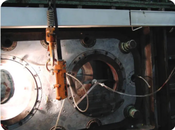
Figure 2 shows the model mounted in test chamber.

Figure 2. Model in test chamber.

Figure 3 shows the rake including fourteen hot wire sensors. The sensors location detail is listed in Table 1. The sensors, 100 micron in diameter and 0.005 m in length, were made of nickel.

(4)

xx/xx

Table 1. Hot wire sensors location.

y/c

Sensor

–0.245 S1

–0.175 S2

–0.140 S3

–0.105 S4

–0.070 S5

–0.035 S6

0 S7

0.035 S8

0.070 S9

0.105 S10

0.140 S11

0.175 S12

0.210 S13

0.245 S14

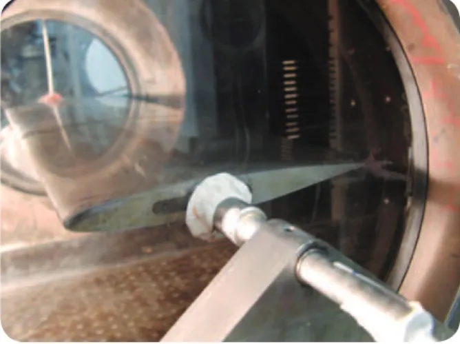
Figure 4 shows the airfoil and the rake inside the test chamber.

Figure 4. Airfoil, rake and sensors fixed in the test chamber.

In order to record hot wire sensors results, Dantec CTA constant temperature system was applied with overheat of 0.8 and a sampling frequency of 1200 kHz. For each sensor, this frequency was taken to be 5 kHz. CTA is Constant Temperature Anemometry.

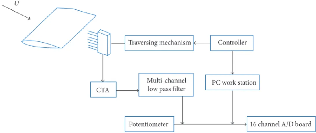
Figure 5 shows the block diagram of data acquisition system.

To eliminate the white noise from results, a low-transition filter was used with a cut-off frequency of 300 Hz considering the PSD of curves and the Weiner method.This method is described in detail by Weiner (1949).

Figure 6 shows the energy level curve for a single hot wire sensor to determine the cut-off frequency.

The oscillation mechanism was capable of pitching the model at various amplitudes, mean incidence angles of attack and oscillation frequencies. Since x/c = 0.4 was the airfoil aerodynamic center, the pitch rotation axis was fixed at the x/c = 0.4 airfoil chord. A hydraulic vibrating system was used to create pitch oscillations that were transmitted to the airfoil through a shaft and extruded from the test chamber window (Fig. 7). The average and instantaneous angle of attack were measured by a linear 0.1° precision potentiometer.

(5)

xx/xx

During the tests, Mach number measurements with maximum calculation error of 1% were obtained by means of a pitot-static tube fixed at model’s upstream. Pressures were measured using differential pressure sensors with a measurement range of up to 15 psi and maximum error of 0.15% span.

Figure 5. Block diagram of data acquisition system.

Figure 6. PSD values of a hot wire.

Traversing mechanism Controller

Multi-channel

low pass ﬁlter PC work station

16 channel A/D board Potentiometer

CTA U

10–8 10–6

100 ₁₀1 ₁₀2 ₁₀3

10–4 10–2 100 102

f (Hz)

P

S

D

Fcut = 300Hz

Figure 7. Hydraulic oscillating alpha-mechanism system.

(6)

xx/xx

The tests error sources included the flow field (both non-uniformity and turbulence level in the wind tunnel), model installation and α-setting, pressure sensors, airfoil model structure, linear potentiometer, A/D range, hot wires, effects of walls and model blockage. According to Amiri et al. (2013), a maximum uncertainty of 4% was calculated.

Wind tunnel was the same for this research and for Amiri’s but the NACA0012 airfoil was chosen in Amiri’s research because its standard experimental data was available for verification and also to evaluate equipment and wind tunnel precision.

NUMERICAL METHOD

The flow structure around a supercritical airfoil was predicted employing Ansys CFX software and the results were compared with experimental tests.

Turbulence model was Shear Stress Transport (SST k-ω), which was proposed by Menter et al. (2003) to combine the precise, powerful k-ω model (for near wall regions where the Reynolds number is low) with free-stream independent k-ε model (for regions far from the walls where the Reynolds number is high).

Two dimensional simulations were applied as the case study was the main goal and to reduce computational costs. In addition, numerical analysis validation in 2D case is confirmed by some references such as Thiery and Coustols (2006) and Ol et al. (2009). Calculation domain was selected by reviewing some references as Moreau et al. (2008) and Ang et al. (2004). Dimensions of domain are considered as 4 times of chord length in front, above, and below the leading edge, and 9 times of chord length behind the trailing edge. Moreover, it is sufficiently distanced from airfoil surface to minimize its influence on the solution.

Geometry and computational domain are shown in Fig. 8.

Figure 8. Computational domain.

L = Chord

9L 4L

4L

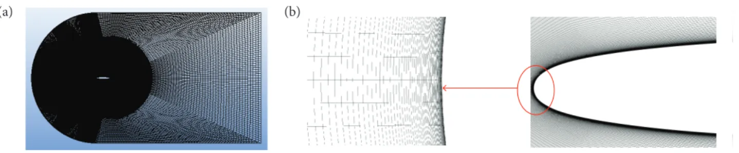
After grid independency, fine grid was used to predict the flow field around Sc(2)0410 airfoil. Total element of grid is 187220 and total node is 376068.

Figure 9 shows the structured grid used to predict the flow field around the airfoil.

Figure 9. (a) Computational grid; (b) close-up view.

(a) (b)

(7)

xx/xx

The time step used in unsteady solutions was 0.0005 s. To achieve stable conditions, simulations were carried out for almost 4200 time steps to pass the inlet flow through the entire computational domain for approximately 7 times. The present results are obtained by statistical time averaging of the last 1800 time steps.

The method validity to reach the stable conditions could be carried out by referring to Moghadam et al. (2016) and Kiani and Javadi (2016).

Boundary conditions include time-independent uniform-velocity profile for inlets and static pressure for outlets. The airfoil surface is assumed to be non-slip and the reference pressure is considered as zero.

GOVERNING EQUATIONS

Governing equations for this problem are conservation of mass, momentum, and energy for the case of unsteady compressible flow as follows:

Continuity (Eq. 1):

x Momentum (Eq. 2):

y Momentum (Eq. 3):

Energy (Eq. 4):

(1) (2) (3) (4) (5) (6) (7) where: 𝐸_𝑡 is the sum of kinetic and internal energy.

The shear stress (𝜏_𝑥𝑦) and normal stress components (𝜏_𝑥𝑥 and 𝜏_𝑦𝑦) can be expressed in terms of velocity gradients as follows:

Shear stress (Eq. 5):

X-normal stress (Eq. 6):

Y-normal stress (Eq. 7):

where: 𝜇 is the dynamic viscosity of the fluid. These equations are described in Detail by Drazin and Riley (2006).

Several researches, as those carried out by Mojiri and Datta (2009) and Eleni et al. (2012), showed that by proper grid generation in boundary layer and Y+_{close to 1, SST k-ω model will give more precise results. SST model was applied here since capturing the} wake was the main goal of the research in which vortex observation, flow behavior close to walls, and boundary layer analysis were to be focused on.

In SST turbulence model, K-ω and K-εare both multiplied by a blending function and then summed. Blending function is designed so that it equals to 1 in near-wall regions (which activates K-ω model in that region) and equals to zero in regions far from the wall (which activates K-ε model in that region). This turbulence model is common for airfoil flow analysis and behaves properly in flow separation and in reverse pressure gradient.

: 𝜕𝜕𝜕𝜕/𝜕𝜕𝜕𝜕+ 𝜕𝜕 /𝜕𝜕𝜕𝜕 (𝜕𝜕𝜌𝜌)+𝜕𝜕/𝜕𝜕𝜕𝜕(𝜕𝜕𝜌𝜌)=0 (1)

: 𝜕𝜕/𝜕𝜕𝜕𝜕(𝜕𝜕𝜌𝜌)+𝜕𝜕/𝜕𝜕𝜕𝜕(𝜕𝜕𝜌𝜌2_{+𝑝𝑝−𝜏𝜏𝜕𝜕𝜕𝜕)+𝜕𝜕/𝜕𝜕𝜕𝜕(𝜕𝜕𝜌𝜌𝜌𝜌−𝜏𝜏𝜕𝜕𝜕𝜕)=0} ₍₂₎

: 𝜕𝜕/𝜕𝜕𝜕𝜕(𝜕𝜕𝜌𝜌)+𝜕𝜕/𝜕𝜕𝜕𝜕(𝜕𝜕𝜌𝜌𝜌𝜌−𝜏𝜏𝜕𝜕𝜕𝜕)+𝜕𝜕/𝜕𝜕𝜕𝜕(𝜕𝜕𝜌𝜌2_{+𝑝𝑝−𝜏𝜏𝜕𝜕𝜕𝜕)=0} ₍₃₎

:

𝜕𝜕/(𝐸𝐸𝜕𝜕)+𝜕𝜕/𝜕𝜕𝜕𝜕[(𝐸𝐸𝜕𝜕+𝑝𝑝)𝜌𝜌+𝑞𝑞𝜕𝜕−𝜌𝜌𝜏𝜏𝜕𝜕𝜕𝜕−𝜌𝜌𝜏𝜏𝜕𝜕𝜕𝜕]+𝜕𝜕/𝜕𝜕𝜕𝜕[(𝐸𝐸𝜕𝜕+𝑝𝑝)𝜌𝜌+𝑞𝑞𝜕𝜕−𝜌𝜌𝜏𝜏𝜕𝜕𝜕𝜕−𝜌𝜌𝜏𝜏𝜕𝜕𝜕𝜕]=0 (4)

𝐸𝐸𝜕𝜕

: 𝜕𝜕𝜕𝜕/𝜕𝜕𝜕𝜕+ 𝜕𝜕 /𝜕𝜕𝜕𝜕 (𝜕𝜕𝜌𝜌)+𝜕𝜕/𝜕𝜕𝜕𝜕(𝜕𝜕𝜌𝜌)=0 (1)

: 𝜕𝜕/𝜕𝜕𝜕𝜕(𝜕𝜕𝜌𝜌)+𝜕𝜕/𝜕𝜕𝜕𝜕(𝜕𝜕𝜌𝜌2_{+𝑝𝑝−𝜏𝜏𝜕𝜕𝜕𝜕)+𝜕𝜕/𝜕𝜕𝜕𝜕(𝜕𝜕𝜌𝜌𝜌𝜌−𝜏𝜏𝜕𝜕𝜕𝜕)=0} ₍₂₎

: 𝜕𝜕/𝜕𝜕𝜕𝜕(𝜕𝜕𝜌𝜌)+𝜕𝜕/𝜕𝜕𝜕𝜕(𝜕𝜕𝜌𝜌𝜌𝜌−𝜏𝜏𝜕𝜕𝜕𝜕)+𝜕𝜕/𝜕𝜕𝜕𝜕(𝜕𝜕𝜌𝜌2_{+𝑝𝑝−𝜏𝜏𝜕𝜕𝜕𝜕)=0} ₍₃₎

:

𝐸𝐸𝜕𝜕

: 𝜕𝜕𝜕𝜕/𝜕𝜕𝜕𝜕+ 𝜕𝜕 /𝜕𝜕𝜕𝜕 (𝜕𝜕𝜌𝜌)+𝜕𝜕/𝜕𝜕𝜕𝜕(𝜕𝜕𝜌𝜌)=0 (1)

: 𝜕𝜕/𝜕𝜕𝜕𝜕(𝜕𝜕𝜌𝜌)+𝜕𝜕/𝜕𝜕𝜕𝜕(𝜕𝜕𝜌𝜌2_{+𝑝𝑝−𝜏𝜏𝜕𝜕𝜕𝜕)+𝜕𝜕/𝜕𝜕𝜕𝜕(𝜕𝜕𝜌𝜌𝜌𝜌−𝜏𝜏𝜕𝜕𝜕𝜕)=0} ₍₂₎

3): 𝜕𝜕/𝜕𝜕𝜕𝜕(𝜕𝜕𝜌𝜌)+𝜕𝜕/𝜕𝜕𝜕𝜕(𝜕𝜕𝜌𝜌𝜌𝜌−𝜏𝜏𝜕𝜕𝜕𝜕)+𝜕𝜕/𝜕𝜕𝜕𝜕(𝜕𝜕𝜌𝜌2+𝑝𝑝−𝜏𝜏𝜕𝜕𝜕𝜕)=0 (3)

:

𝐸𝐸𝜕𝜕

: 𝜕𝜕𝜕𝜕/𝜕𝜕𝜕𝜕+ 𝜕𝜕 /𝜕𝜕𝜕𝜕 (𝜕𝜕𝜌𝜌)+𝜕𝜕/𝜕𝜕𝜕𝜕(𝜕𝜕𝜌𝜌)=0 (1)

: 𝜕𝜕/𝜕𝜕𝜕𝜕(𝜕𝜕𝜌𝜌)+𝜕𝜕/𝜕𝜕𝜕𝜕(𝜕𝜕𝜌𝜌2_{+𝑝𝑝−𝜏𝜏𝜕𝜕𝜕𝜕)+𝜕𝜕/𝜕𝜕𝜕𝜕(𝜕𝜕𝜌𝜌𝜌𝜌−𝜏𝜏𝜕𝜕𝜕𝜕)=0} ₍₂₎

: 𝜕𝜕/𝜕𝜕𝜕𝜕(𝜕𝜕𝜌𝜌)+𝜕𝜕/𝜕𝜕𝜕𝜕(𝜕𝜕𝜌𝜌𝜌𝜌−𝜏𝜏𝜕𝜕𝜕𝜕)+𝜕𝜕/𝜕𝜕𝜕𝜕(𝜕𝜕𝜌𝜌2_{+𝑝𝑝−𝜏𝜏𝜕𝜕𝜕𝜕)=0} ₍₃₎

:

𝐸𝐸𝜕𝜕

𝜏𝜏𝑥𝑥𝑥𝑥 𝜏𝜏𝑥𝑥𝑥𝑥 𝜏𝜏𝑥𝑥𝑥𝑥

5): 𝜏𝜏𝑥𝑥𝑥𝑥=𝜏𝜏𝑥𝑥𝑥𝑥=𝜇𝜇 (𝜕𝜕u/𝜕𝜕y +𝜕𝜕𝜕𝜕/) (5)

: 𝜆𝜆 (∇.V)+2𝜇𝜇 𝜕𝜕𝜕𝜕/𝜕𝜕𝑥𝑥 (6)

: 𝜆𝜆 (𝛻𝛻.𝑉𝑉)+2𝜇𝜇 𝜕𝜕𝜕𝜕/𝜕𝜕𝑥𝑥 (7)

𝜇𝜇

ω

ω ɛ

ω

: 𝜏𝜏𝑥𝑥𝑥𝑥=𝜏𝜏𝑥𝑥𝑥𝑥=𝜇𝜇 (𝜕𝜕u/𝜕𝜕y +𝜕𝜕𝜕𝜕/) (5)

. 6): 𝜆𝜆 (∇.V)+2𝜇𝜇 𝜕𝜕𝜕𝜕/𝜕𝜕𝑥𝑥 (6)

: 𝜆𝜆 (𝛻𝛻.𝑉𝑉)+2𝜇𝜇 𝜕𝜕𝜕𝜕/𝜕𝜕𝑥𝑥 (7)

𝜇𝜇

ω

ω ɛ

ω

: 𝜏𝜏𝑥𝑥𝑥𝑥=𝜏𝜏𝑥𝑥𝑥𝑥=𝜇𝜇 (𝜕𝜕u/𝜕𝜕y +𝜕𝜕𝜕𝜕/) (5)

: 𝜆𝜆 (∇.V)+2𝜇𝜇 𝜕𝜕𝜕𝜕/𝜕𝜕𝑥𝑥 (6)

. 7): 𝜆𝜆 (𝛻𝛻.𝑉𝑉)+2𝜇𝜇 𝜕𝜕𝜕𝜕/𝜕𝜕𝑥𝑥 (7)

𝜇𝜇

ω

ω ɛ

ω

(8)

xx/xx

Equations applied for such turbulence model are as follows (Eq. 8):

(8) (9) (10) (11) ɛ 𝜕𝜕(𝜌𝜌𝜌𝜌)

𝜕𝜕𝜕𝜕 +𝜕𝜕(𝜌𝜌𝑈𝑈L𝜌𝜌)𝜕𝜕𝑥𝑥L = 𝑃𝑃NO− 𝛽𝛽∗𝜌𝜌𝜌𝜌𝜌𝜌 +_{𝜕𝜕𝑥𝑥L}𝜕𝜕 S(𝜇𝜇 + 𝜎𝜎O𝜇𝜇U)_{𝜕𝜕𝑥𝑥L}𝜕𝜕𝜌𝜌V W(X#)

WU + W(X&Y#)

WZY = 𝛼𝛼𝜌𝜌𝑆𝑆%− 𝛽𝛽𝜌𝜌𝜌𝜌%+ W

WZY](𝜇𝜇 + 𝜎𝜎#𝜇𝜇U) W#

WZY^ + 2(1 − 𝐹𝐹`)𝜌𝜌𝜎𝜎#% ` # WO WZY W# WZY

𝐹𝐹`= tanh efmin i𝑚𝑚𝑚𝑚𝑥𝑥 l_𝛽𝛽√𝜌𝜌_∗_{𝜌𝜌𝜔𝜔 .}500𝜈𝜈_𝜔𝜔_%_{𝜌𝜌 o .}4𝜌𝜌𝜎𝜎#%𝜌𝜌_{𝐶𝐶𝐶𝐶O#𝜔𝜔}_%rs t

u

𝐶𝐶𝐶𝐶O#= max w2𝜌𝜌𝜎𝜎#%_#`_WZYWO_WZYW#. 10x`y_z

𝜈𝜈U =_{}~({|#.ÄÅÇ)}{|O ; 𝜈𝜈U=ÑÖ_X

ɛ

𝜕𝜕(𝜌𝜌𝜌𝜌)

𝜕𝜕𝜕𝜕 +

𝜕𝜕(𝜌𝜌𝑈𝑈

L

𝜌𝜌)

𝜕𝜕𝑥𝑥

L

= 𝑃𝑃N

O

− 𝛽𝛽

∗

_{𝜌𝜌𝜌𝜌𝜌𝜌 +}

𝜕𝜕

𝜕𝜕𝑥𝑥

L

S(𝜇𝜇 + 𝜎𝜎

O

𝜇𝜇

U

)

𝜕𝜕𝜌𝜌

𝜕𝜕𝑥𝑥

L

V

W(X#)

WU

+

W(X&Y#)

WZY

= 𝛼𝛼𝜌𝜌𝑆𝑆

%

_{− 𝛽𝛽𝜌𝜌𝜌𝜌}

%

₊

W

WZY

](𝜇𝜇 + 𝜎𝜎

#

𝜇𝜇

U

)

W#

WZY

^ + 2(1 − 𝐹𝐹

`

)𝜌𝜌𝜎𝜎

#%

` # WO WZY W# WZY

(8)

𝐹𝐹

`

= tanh efmin i𝑚𝑚𝑚𝑚𝑥𝑥 l

_𝛽𝛽

√𝜌𝜌

_∗

_{𝜌𝜌𝜔𝜔 .}

500𝜈𝜈

_𝜔𝜔

_%

_{𝜌𝜌 o .}

4𝜌𝜌𝜎𝜎

_{𝐶𝐶𝐶𝐶}

#%

𝜌𝜌

O#

𝜔𝜔

%

rs

t

u

𝐶𝐶𝐶𝐶

O#

= max w2𝜌𝜌𝜎𝜎

#%_#`_WZWO_Y_WZW#_Y

. 10

x`y

z

𝜈𝜈

U

=

_}~({{|O_|_#.ÄÅ_Ç₎

; 𝜈𝜈

U

=

ÑÖ_X ɛ

𝜕𝜕(𝜌𝜌𝜌𝜌) 𝜕𝜕𝜕𝜕 +

𝜕𝜕(𝜌𝜌𝑈𝑈L𝜌𝜌)

𝜕𝜕𝑥𝑥L = 𝑃𝑃NO− 𝛽𝛽

∗_{𝜌𝜌𝜌𝜌𝜌𝜌 +} 𝜕𝜕

𝜕𝜕𝑥𝑥LS(𝜇𝜇 + 𝜎𝜎O𝜇𝜇U) 𝜕𝜕𝜌𝜌 𝜕𝜕𝑥𝑥LV W(X#)

WU + W(X&Y#)

WZY = 𝛼𝛼𝜌𝜌𝑆𝑆%− 𝛽𝛽𝜌𝜌𝜌𝜌%+ W

𝐹𝐹`= tanh efmin i𝑚𝑚𝑚𝑚𝑥𝑥 l_𝛽𝛽√𝜌𝜌_∗_{𝜌𝜌𝜔𝜔 .}500𝜈𝜈_𝜔𝜔_%_{𝜌𝜌 o .}_{𝐶𝐶𝐶𝐶}4𝜌𝜌𝜎𝜎#%𝜌𝜌 O#𝜔𝜔%rs

t u

𝐶𝐶𝐶𝐶O#= max w2𝜌𝜌𝜎𝜎#%_#`_WZYWO_WZYW#. 10x`yz

𝜈𝜈U =_}~({|#.ÄÅ{|O _Ç) ; 𝜈𝜈U=ÑÖ_X ɛ

𝜕𝜕(𝜌𝜌𝜌𝜌) 𝜕𝜕𝜕𝜕 +

𝜕𝜕(𝜌𝜌𝑈𝑈L𝜌𝜌)

𝜕𝜕𝑥𝑥L = 𝑃𝑃NO− 𝛽𝛽∗𝜌𝜌𝜌𝜌𝜌𝜌 + 𝜕𝜕

𝜕𝜕𝑥𝑥LS(𝜇𝜇 + 𝜎𝜎O𝜇𝜇U) 𝜕𝜕𝜌𝜌 𝜕𝜕𝑥𝑥LV W(X#)

WU + W(X&Y#)

WZY = 𝛼𝛼𝜌𝜌𝑆𝑆

%_{− 𝛽𝛽𝜌𝜌𝜌𝜌}%₊ W

𝐹𝐹`= tanh efmin i𝑚𝑚𝑚𝑚𝑥𝑥 l_𝛽𝛽√𝜌𝜌∗_{𝜌𝜌𝜔𝜔 .} 500𝜈𝜈

𝜔𝜔%_{𝜌𝜌 o .}

4𝜌𝜌𝜎𝜎#%𝜌𝜌 𝐶𝐶𝐶𝐶O#𝜔𝜔%rs

t u

𝐶𝐶𝐶𝐶O#= max w2𝜌𝜌𝜎𝜎#%_#`_WZWO_Y_WZW#_Y. 10x`yz 9)

𝜈𝜈U= {|O

}~({|#.ÄÅÇ) ; 𝜈𝜈U= ÑÖ

X

ɛ

𝜕𝜕(𝜌𝜌𝜌𝜌)

𝜕𝜕𝜕𝜕 +

𝜕𝜕(𝜌𝜌𝑈𝑈

L

𝜌𝜌)

𝜕𝜕𝑥𝑥

L

= 𝑃𝑃N

O

− 𝛽𝛽

∗

_{𝜌𝜌𝜌𝜌𝜌𝜌 +}

𝜕𝜕

𝜕𝜕𝑥𝑥

L

S(𝜇𝜇 + 𝜎𝜎

O

𝜇𝜇

U

)

𝜕𝜕𝜌𝜌

𝜕𝜕𝑥𝑥

L

V

W(X#)

WU

+

W(X&Y#)

WZY

= 𝛼𝛼𝜌𝜌𝑆𝑆

%

_{− 𝛽𝛽𝜌𝜌𝜌𝜌}

%

₊

W

WZY

](𝜇𝜇 + 𝜎𝜎

#

𝜇𝜇

U

)

W#

WZY

^ + 2(1 − 𝐹𝐹

`

)𝜌𝜌𝜎𝜎

#%

` # WO WZY W# WZY

𝐹𝐹

`

= tanh efmin i𝑚𝑚𝑚𝑚𝑥𝑥 l

_𝛽𝛽

√𝜌𝜌

_∗

_{𝜌𝜌𝜔𝜔 .}

500𝜈𝜈

_𝜔𝜔

_%

_{𝜌𝜌 o .}

_{𝐶𝐶𝐶𝐶}

4𝜌𝜌𝜎𝜎

#%

𝜌𝜌

O#

𝜔𝜔

%

rs

t

u

𝐶𝐶𝐶𝐶

O#

= max w2𝜌𝜌𝜎𝜎

#%_#`_WZWO

Y W# WZY

. 10

x`y

_z

𝜈𝜈

U

=

_}~({|#.ÄÅ{|O _Ç₎

; 𝜈𝜈

U

=

Ñ_XÖ

(10)

𝐹𝐹

%

= tanh Ü]𝑚𝑚𝑚𝑚𝑚𝑚 w

_á%√O∗_#à

.

âyyä_àÇ_#

z^

%

ã

(11)

ć

where the F₁ blending function is (Eq. 9):

where y is the distance from closest wall.

Turbulence viscosity is defined as follows (Eq. 10):

where: S is the shear stress value and F₂ is the second blending function that is defined as follows (Eq. 11):

This method is described in detail by Menter et al. (1993,1994). Figure 10 shows the calculated Y+_{in airfoil wall simulation.}

Figure 10. Y+_{calculated on the airfoil wall.}

1.064e+000

7.984e–001

5.322e–001

2.661e–001

0.000e+000

High-resolution second order upwind method was used for numerical solution of partial differential equations where high accuracy was required in the presence of shocks or discontinuities.

(9)

xx/xx

RESULTS

All tests were carried out under static and dynamic conditions both experimentally and numerically. Velocity profiles, Mach contours, statistical and frequency analysis of hot wire outputs were used to identify the wake behavior.

The research results are categorized in two sections: statistical and frequency analysis of hot wire sensors voltages and velocity profiles (derived from calibration).

Before exploring the mentioned parts, it is preferred to show the lift coefficient diagrams in Figs. 11 and 12 for flows with Mach numbers of 0.4 and 0.6, which are sketched to prove the results consistency between numerical analysis and experimental tests, and also to determine the angle of static stall.

Figure 11. Lift coefficient distribution, Mach = 0.4.

Figure 12. Lift coefficient distribution, Mach = 0.6.

-2 0 2 4 6 8 10

-0.2 0 0.2 0.4 0.6 0.8 1 1.2

Alpha

cl

CFD

EXP

-2 0 2 4 6 8

-0.2 0 0.2 0.4 0.6 0.8 1 1.2

Alpha

cl

CFD

EXP

As it is shown in Figs. 5 and 6, the angle of static stall for Mach number of 0.4 is 9° and for Mach number of 0.6 is 7°. Therefore, experimental tests are carried out below stall angle for both Mach numbers of 0.4 and 0.6; a near stall state occurs only in the case of 0.6, oscillation amplitude of 3° and mean angle of attack of 3°.

STATISTICAL AND FREQUENCY ANALYSIS OF HOT WIRE SENSORS VOLTAGES

Results in this section show that the study of wake and its thickness in various cases are possible by statistical and frequency analysis of hot wires output voltages.

(10)

xx/xx

Static Part

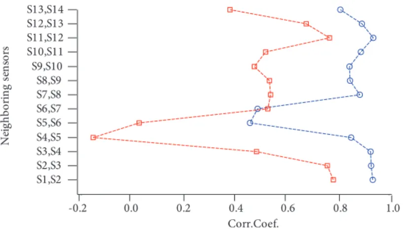
Figure 13 indicates linear correlation coefficient diagram for hot wire sensors.Correlation coefficient is a value between +1 and −1 calculated so as to represent the linear interdependence of two variables or sets of data. Therefore, in this research, correlation coefficient between two adjacentsensors shows the flow behavior at sensor locations. As it is shown in Fig. 13, the coefficient is maximized for a couple of sensors located outside the wake and decreases when they are not at the same region (i.e., one sensor locates inside the wake region and the other locates outside).

Figure 13. Linear correlation coefficient diagram for hot wire sensors.

-0.2 0.0 0.2 0.4 0.6 0.8 1.0

S1,S2 S2,S3 S3,S4 S4,S5 S5,S6 S6,S7 S7,S8 S8,S9 S9,S10 S10,S11 S11,S12 S12,S13 S13,S14

Corr.Coef.

N

ei

g

hb

o

ri

n

g

s

en

so

rs

AOA = 4° AOA = 8°

For angle of 4° for example, sensor S6 achieves minimum correlation with S7 and S5 since it is located inside the wake at the mentioned angle. This also occurs for sensor S5 at angle of 8°.

As mentioned before, the wake region could be estimated by depicting the Correlation coefficient parameter for adjacent sensors and studying their behavior.

Figure 14 shows the time history of hot wires signals at AOA = 4°; qualitative investigation of signals reveals that the wake sensor fluctuations are by far higher than those of other sensors; therefore, the wake location determination becomes possible through a voltage qualitative investigation.

Figure 14. Time history of hot wires output signals at AOA = 4°.

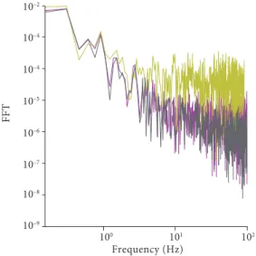
As suggested before, entry of one sensor into the wake region could be observed by means of signal analysis of the sensor voltage. Signal energy or PSD is also a significant parameter. Energy level for angles of attack of 3° and 6° are shown in Figs. 15 and 16 for three sensors located at y/c = 0, y/c = –0.035, and y/c = –0.07.

0 0.5 1.0 1.5 2.0 2.5 3.0 3.5 4.0 Time(s)

(11)

xx/xx

As observed in Figs. 15 and 16, S6 sensor gains maximum energy level by entering the wake region at angle of 3°, whereas, at angle of 6°, by entry of S5 sensor into the region, it gains the maximum energy level and S6 sensor scores the second place.

Dynamic Part

Focus in this section is on the airfoil wake in a pitch sinusoidal motion. Figure 17 shows the instantaneous voltages of three sensors in α(t) = 3 + 3 sin (2πt/T – π/2) pitch oscillation motion at frequency of 3 Hz. Comparing consecutive cycles reveals their repeatability with an appropriate precision; if a complete cycle is considered as a pitch up-pitch down sequence, then every sensor will cover the same pattern through all cycles. Deviations may appear only in very small fluctuations, which are likely related to noise or any other unsteadiness that may instantaneously and irregularly affect the sensors voltages, but not to the flow physics.

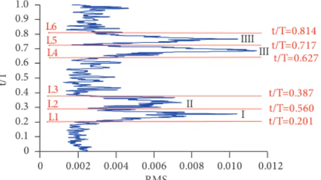
Figure 18 shows the RMS variations in a complete cycle. Lines L1, L2, and L3 in a pitch up, are related to states when the wake enters y/c = 0.0, minimum voltage level, and when the wake leaves that point, respectively. Lines L4, L5, and L6 show the same states in a pitch down. Related times are printed against each line.

10–9

100 ₁₀1 ₁₀2

10–8

10–7

10–6

10–5

10–4

Frequency (Hz)

FF

T

S5 S6 S7 10–2

10–8

100 ₁₀1 ₁₀2

10–7

10–6

10–5

10–4

10–3

Frequency (Hz)

FF

T

S5 S6 S7 10–2

Figure 15. Sensors energy level at angle of attack of 3°.

Figure 16. Sensors energy level at angle of attack of 6°.

(12)

xx/xx

RMS value for each signal increases with an increase in randomness and in amplitude of oscillations around the average value; hence, RMS could be considered equivalent to turbulence intensity in the flow. Variations in Fig. 18 confirm this equivalency; when the sensor enters the wake at L1, RMS value starts increasing and reaches its maximum at point I, then it starts to decrease, getting an extremum at L2, where the voltage is minimum. Afterwards, it starts to increase again, goes up to point II, and finally falls down by getting close to the boundary layer border. Similar behavior is observed in a pitch down.

Figure 19 shows the coefficient of linear correlation between two sensors at y/c = 0.0 (inside the wake) and at y/c = 0.245 (outside the wake). The coefficient of correlation between S7 and the flow outside the wake does not decrease immediately after the sensor locates inside the wake; rather, it decreases remarkably when it gets close to the minimum voltage zone and finally reaches a value of about –0.9 at L2.

Analysis of results from Figs. 13 to 19 confirms that the study of wake is possible by means of sensor voltage analysis even for oscillating airfoil.

Figure 17. Instantaneous voltages of three sensors, pitch oscillation α(t) = 3 + 3 sin (2πt/T – π/2), frequency = 3Hz, Mach = 0.4.

Figure 18. RMS variations in a complete cycle.

Figure 19. Coefficient of linear correlation between sensors S7 and S14. Pitch Up

Pitch Down

y/c=-0.07 y/c=-0.035 y/c=0 α_(t)

0 0.002 0.004 0.006 0.008 0.010 0.012 0

0.1 0.2 0.3 0.4 0.5 0.6 0.7 0.8 0.9 1.0

RMS

t/

T

y/c=0

t/T=0.814

t/T=0.387 t/T=0.560 t/T=0.201 L1

L2 L3 L4 L5 L6

I II

t/T=0.627 t/T=0.717

III IIII

–1.0 –0.6 –0.2 0.2 0.6 1.0 0

0.1 0.2 0.3 0.4 0.5 0.6 0.7 0.8 0.9 1.0

Corr. Coeﬀ.

t/

T t/T

y/c = 0.0 & y/c = -0.245

L1 L2 L3 L4 L5

L6 t/T = 0.814

t/T = 0.717 t/T = 0.627

(13)

xx/xx

VELOCITY PROFILES

Voltage calibration for hot wire sensors was carried out in this research and wake velocity profiles were obtained from hot wire anemometry.

Calibration

According to Motallebi (1994), in high speed flow, due to the compressibility effects, the anemometer is affected not only by changes in flow velocity, but also by density and temperature fluctuations. In other words, for a single normal wire, the output voltage of anemometer is a function of flow velocity, flow density and total temperature (Eq. 12).

(12)

(13)

(14)

(15)

(16) This equation can be written as (Eq. 13):

𝐸𝐸 = 𝐸𝐸(𝑈𝑈. 𝜌𝜌. 𝑇𝑇) (12)

𝐿𝐿𝐿𝐿𝐿𝐿ó𝐸𝐸%_{− 𝐸𝐸y}%_{ò = 𝑆𝑆ôLog(U) + SüLog(ρ) + 𝑆𝑆°Log(T) + 𝑐𝑐𝐿𝐿𝑐𝑐𝑐𝑐𝑐𝑐}

ρ

𝑆𝑆¶=ß[®©™ó´

Ç_x´_¨Ç_ò]

ß[®©™(≠)]

𝑆𝑆ü=ß[®©™ó´

Ç_x´_¨Ç_ò]

ß[®©™(ü)]

ρ

𝑆𝑆é=ß[®©™ó´

Ç_x´_¨Ç_ò]

ß[®©™(é)]

ρ

-

𝐿𝐿𝐿𝐿𝐿𝐿ó𝐸𝐸

%

_{− 𝐸𝐸}

y%

ò = 𝑆𝑆

ô

Log(U) + S

ü

Log(ρ) + 𝑆𝑆

°

Log(T) + 𝑐𝑐𝐿𝐿𝑐𝑐𝑐𝑐𝑐𝑐

ρ

𝑆𝑆

¶

=

ß[®©™ó´ Ç_x´_¨Ç_ò] ß[®©™(≠)]

14)

𝑆𝑆

ü

=

ß[®©™ó´ Ç_x´_¨Ç_ò] ß[®©™(ü)]

ρ

𝑆𝑆

é

=

ß[®©™ó´ Ç_x´_¨Ç_ò] ß[®©™(é)]

ρ

-

𝐿𝐿𝐿𝐿𝐿𝐿ó𝐸𝐸

%

_{− 𝐸𝐸}

y%

ò = 𝑆𝑆

ô

Log(U) + S

ü

Log(ρ) + 𝑆𝑆

°

Log(T) + 𝑐𝑐𝐿𝐿𝑐𝑐𝑐𝑐𝑐𝑐

ρ

𝑆𝑆

¶

=

𝑆𝑆

ü

=

15)

ρ

𝑆𝑆

é

=

ρ

-

𝐿𝐿𝐿𝐿𝐿𝐿ó𝐸𝐸

%

_{− 𝐸𝐸}

y%

ò = 𝑆𝑆

ô

Log(U) + S

ü

Log(ρ) + 𝑆𝑆

°

Log(T) + 𝑐𝑐𝐿𝐿𝑐𝑐𝑐𝑐𝑐𝑐

ρ

𝑆𝑆

¶

=

𝑆𝑆

ü

=

ρ

𝑆𝑆

é

=

16)

ρ

-

If ρ and T are constants (Eq. 14):

If U and T are constants (Eq. 15):

If ρand U are constants (16):

Therefore, several tests shall be necessary to calibrate sensor’s output and its conversion into velocity. Those tests require to obtain S_u by velocity variation while temperature and density are constants. Also to obtain S_ρ by density variation while temperature and velocity are constants and to obtain S_T by temperature variation while velocity and density are constants.

Generally, experimental calculation of calibration coefficients could be achieved by two methods: • Direct experimental method

• Indirect or semi-experimental method

In direct method, hot wire is placed in free stream of tunnel and the stagnation pressure is varied while the Mach number and stagnation temperature are kept unchanged. By time averaging, it is then possible to obtain the mean output voltage of the anemometer as a function of mean mass flux.

The slope of a plot of ln (E) versus ln (ru) will determine De_ru. The De_Tosensitivity coefficient can be determined by a controlled change of gas total temperature while gas density and velocity are kept unchanged. This method is not practiced in conventional wind tunnels, since it requires several tests in special tunnels.

When the possibility of calibrating the hot wire in a controlled flow environment is not feasible in a given test facility, then it is advisable to calibrate the hot wire in wind tunnel by simultaneous variation of density, velocity and temperature.

An indirect calibration method is employed in this research, which was first introduced by Stainback and Nagabushana (1993) and Stainback et al. (1983). Applying the mentioned method they calculated, at first, the calibration coefficients by several tests in wind tunnel, and then estimated a statistically optimized equation (Eq. 17):

(14)

xx/xx

(17)

(18)

(19)

(20)

log(E) = 𝐴𝐴`+ 𝐴𝐴%log (u) + 𝐴𝐴±log (r) + 𝐴𝐴tlog (𝑻𝑻𝑻𝑻) + 𝐴𝐴âlog (u) log (r) + 𝐴𝐴¥log (u) log (𝑻𝑻𝑻𝑻)

+ 𝐴𝐴µlog (r_{) log (𝑻𝑻𝑻𝑻) + 𝐴𝐴∂log (u) log (}r_{) log (𝑻𝑻𝑻𝑻)}

𝑆𝑆ô= 𝐴𝐴%+ 𝐴𝐴â(logr_{) + 𝐴𝐴¥log (𝑻𝑻𝑻𝑻) + 𝐴𝐴∂ log (}r_{) ln (𝑻𝑻𝑻𝑻)}

𝑆𝑆r= 𝐴𝐴±+ 𝐴𝐴âlog (u) + 𝐴𝐴µ log (𝑻𝑻𝑻𝑻) + 𝐴𝐴∂ log (u) log (𝑻𝑻𝑻𝑻))

𝑆𝑆°∑= 𝐴𝐴t+ 𝐴𝐴¥log (u) + 𝐴𝐴µ log (r) + 𝐴𝐴∂ log (u) log (r)

+ 𝐴𝐴µlog (r_{) log (𝑻𝑻𝑻𝑻) + 𝐴𝐴∂log (u) log (}r_{) log (𝑻𝑻𝑻𝑻)}

18)

log(E) = 𝐴𝐴`+ 𝐴𝐴%log (u) + 𝐴𝐴±log (r_{) + 𝐴𝐴tlog (𝑻𝑻𝑻𝑻) + 𝐴𝐴âlog (u) log (}r_{) + 𝐴𝐴¥log (u) log (𝑻𝑻𝑻𝑻)}

+ 𝐴𝐴µlog (r) log (𝑻𝑻𝑻𝑻) + 𝐴𝐴∂log (u) log (r) log (𝑻𝑻𝑻𝑻)

𝑆𝑆ô = 𝐴𝐴%+ 𝐴𝐴â(logr) + 𝐴𝐴¥log (𝑻𝑻𝑻𝑻) + 𝐴𝐴∂ log (r) ln (𝑻𝑻𝑻𝑻)

(19)

𝑆𝑆°∑= 𝐴𝐴t+ 𝐴𝐴¥log (u) + 𝐴𝐴µ log (r_{) + 𝐴𝐴∂ log (u) log (}r₎

log(E) = 𝐴𝐴`+ 𝐴𝐴%log (u) + 𝐴𝐴±log (r_{) + 𝐴𝐴tlog (𝑻𝑻𝑻𝑻) + 𝐴𝐴âlog (u) log (}r_{) + 𝐴𝐴¥log (u) log (𝑻𝑻𝑻𝑻)}

𝑆𝑆°∑= 𝐴𝐴t+ 𝐴𝐴¥log (u) + 𝐴𝐴µ log (r_{) + 𝐴𝐴∂ log (u) log (}r₎

20)

Equations for sensitivity coefficients are as follows (Eqs. 18, 19, and 20):

In this research, output voltages for each sensor were obtained for eight values of Mach number during several tests in wind tunnel. Fourteen sensors mounted on a rake were placed in wind tunnel for data sampling in various Mach numbers. Mach number varied from 0.35 to 0.75 and sensors outputs were recorded by sampling frequency of 5 kHz.

Obtaining output voltages, a system of equations comprising eight equations and eight unknowns was configured and solved to give the coefficients A₁ to A₈. Equations 18 to 20, for sensitivity coefficients, were solved to give S_u, S_ρ, and S_To, consequently. Applying these coefficients in tests helped to benefit from converting the voltage into velocity.

Static Part

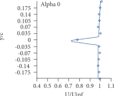
Figures 20 to 22 show the velocity diagrams in wake region for Mach number of 0.4 at downstream distance of 0.25 chord. A significant velocity decrease in wake region is obvious in diagrams. Location of maximum velocity reduction shifts downward as AOA increases. S7 sensor indicates maximum voltage reduction at angle of 0°, which suggests minimum velocity in turn. Mentioned sensor leaves the wake region as the angle of attack varies from 0° to 3° and S6 sensor indicates the minimum velocity instead. That means the wake tends downward.

S5 sensor also enters the wake region by increasing the angle of attack to 6°, which indicates a large velocity reduction. The wake thickness increases at this angle of attack and both S5 and S6 sensors are placed inside the wake region.

Figures 23 to 25 show the velocity diagrams in wake region for Mach number of 0.6 at downstream distance of 0.25 chord. Velocity reduction is observed in the wake. Like in the previous case, the wake rotates clockwise by increasing the angle of attack. Wake thickness and velocity reduction at Mach number of 0.6 is more than those of flow with Mach number of 0.4. This is obvious by comparing Figs. 22 and 25.

Velocity behavior at x/c = 0.5 is almost similar to that of x/c = 0.25, as shown in Fig. 26; deviations are the rate and slope of voltage reduction which is higher at x/c = 0.25, and the wake thickness which is greater at x/c = 0.5. This is a result of wake effect weakening as departing longitudinally from airfoil.

Figure 20. Streamwise velocity profile at x/c = 0.25, Mach = 0.4.

0.4 0.5 0.6 0.7 0.8 0.9 1 1.1

-0.175-0.14

-0.105 -0.07 -0.035 0

0.0350.07

0.105 0.14 0.175

U/Uinf

y/c

Exp CFD Alpha 0

(15)

xx/xx

0.4 0.5 0.6 0.7 0.8 0.9 1 1.1 -0.175

-0.14 -0.105-0.07 -0.035 0 0.035 0.07 0.1050.14 0.175

U/Uinf

y/c

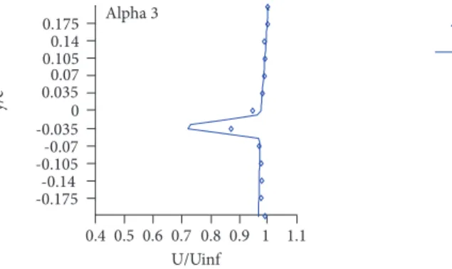
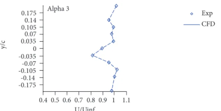
Exp CFD Alpha 3

0.4 0.5 0.6 0.7 0.8 0.9 1 1.1

-0.175-0.14

-0.105 -0.07 -0.035 0

0.0350.07

0.105 0.14 0.175

U/Uinf

y/c

Exp CFD Alpha 6

0.4 0.5 0.6 0.7 0.8 0.9 1 1.1

-0.175-0.14

-0.105-0.07

-0.035 0

0.0350.07

0.1050.14

0.175

U/Uinf

y/c

Exp CFD Alpha 0

0.4 0.5 0.6 0.7 0.8 0.9 1 1.1 -0.175-0.14

-0.105-0.07 -0.035 0 0.0350.07 0.1050.14 0.175

U/Uinf

y/c

Exp CFD Alpha 3

(16)

xx/xx

Figure 27. Streamwise velocity profile, pitch motion α(t) = 3 + 3 sin(wt), frequency = 3 Hz, Mach = 0.4.

0.4 0.5 0.6 0.7 0.8 0.9 1 1.1 -0.175-0.14

-0.105-0.07 -0.035 0 0.0350.07 0.105 0.14 0.175

U/Uinf

y/c

Exp CFD

Alpha 6

0.4 0.5 0.6 0.7 0.8 0.9 1 1.1 -0.175-0.14

-0.105-0.07 -0.035 0 0.0350.07 0.1050.14 0.175

U/Uinf

y/c

Exp CFD

Alpha 0

0.4 0.5 0.6 0.7 0.8 0.9 1 1.1 -0.175-0.14

-0.105-0.07 -0.035 0 0.0350.07 0.105 0.14 0.175

U/Uinf

y/c

Exp CFD

Alpha 3

As observed from velocity profiles, results obtained from both experimental and numerical analysis are in a good consistence.

Dynamic Part

Figures 27 to 30 show the wake velocity profiles in α(t) = 3 + 3 sin(wt) pitch oscillation. In order to achieve velocity profiles for oscillating airfoil, output signal for each sensor was recorded at each instantaneous angle of attack and averaged for 15 complete oscillating cycles.

At angle of attack of 3°, S6 and S7 sensors are both placed in wake region, while at angle of attack of 6°, S5 sensor indicates velocity reduction from free stream velocity, which implies a notable increase of wake thickness.

As observed from velocity profiles, the wake rotates clockwise and tends downward by increasing the angle of attack. At angle of attack of 3°, S6 sensor shows a velocity decrease, while at 6° the wake tends down and S5 sensor shows a velocity decrease instead. Wake thickness also increases due to flow separation at trailing edge and rise of a shock on the airfoil.

(17)

xx/xx

Figure 30. Streamwise velocity profile, pitch motion α(t) = 3 + 3 sin(wt), frequency = 3 Hz, Mach = 0.6. 0.4 0.5 0.6 0.7 0.8 0.9 1 1.1

-0.175-0.14 -0.105-0.07 -0.035 0 0.0350.07 0.1050.14 0.175

U/Uinf

y/c

Exp CFD

Alpha 6

0.4 0.5 0.6 0.7 0.8 0.9 1 1.1 -0.175-0.14

-0.105 -0.07 -0.035 0 0.0350.07 0.105 0.14 0.175

U/Uinf

y/c

Exp CFD Alpha 3

0.4 0.5 0.6 0.7 0.8 0.9 1 1.1 -0.175-0.14

-0.105 -0.07 -0.035 0 0.0350.07 0.105 0.14 0.175

U/Uinf

y/c

Exp CFD

Alpha 6

This could be observed and validated by Mach contours obtained from numerical solution that are shown in Figs. 32 to 35. Figure 31 shows the pressure coefficient diagram on airfoil surface for angles of 3.8° and 4° in a pitch up motion. The diagram indicates a shock for angles beyond 4°.

A shock occurs on the airfoil for angles above 4°. This is also noticeable by studying the Mach number contours for oscillating airfoil.

As indicated in the diagrams, the vortex created at leading edge moves towards trailing edge by increasing the angle of attack and finally sheds from trailing edge into the wake.

Maximum oscillation of 6° stays far from stall since static stall angle for a flow with Mach number of 0.4 is 9°, as described in lift coefficient diagrams. Although at Mach number of 0.4, separation occurs at trailing edge by increase in oscillation angle, but the airfoil would not experience a shallow stall.

In a flow with Mach number of 0.6, static stall angle is 7°. Oscillating shock occurs on the airfoil in this case, which shows a shallow stall.

(18)

xx/xx

0 0.1 0.2 0.3 0.4 0.5 0.6 0.7 0.8 0.9 1 -3

-2.5 -2 -1.5 -1 -0.5 0 0.5 1 1.5

x/c

Cp

αup = 4 αup = 3.8

Cp critical =-1.29

a a

Figure 31. Pressure Coefficient distribution over the airfoil obtained from numerical solution, Mach = 0.6.

Figure 32. Mach contour, pitch motion α(t) = 3 + 3 sin(wt), frequency = 3 Hz, Mach = 0.4, Alpha = 5°.

Figure 33. Mach contour, pitch motion α(t) = 3 + 3 sin(wt), frequency = 3 Hz, Mach = 0.4, Alpha = 6°

α

w

α

w

α

w

(19)

xx/xx

α w

α

w

α

w

α

w

Figure 34. Mach contour, pitch motion α(t) = 3 + 3 sin(wt), frequency = 3 Hz, Mach = 0.6, Alpha = 5°.

Figure 35. Mach contour, pitch motion α(t) = 3 + 3 sin(wt), frequency = 3 Hz, Mach = 0.6, Alpha = 6º.

Finally, by moving downward and decreasing the angle of attack, the separated flow reattaches to the airfoil surface for both Mach numbers of 0.4 and 0.6.

CONCLUSION

Wake of a supercritical airfoil in a pitching motion was investigated experimentally and numerically in case of compressible flow. Static stall angle was obtained for Mach numbers of 0.4 and 0.6 by lift coefficient diagram in both experimental and numerical cases. Moreover, results consistency for both cases was indicated by lift coefficient diagram.

By depicting sensors output diagrams like RMS, time history, correlation coefficient and energy level, it was shown that the wake investigation and its behavior in compressible flow could be achieved by frequency and statistical analysis of sensors voltages if the precise velocity value does not matter.

Calibration was carried out despite the troubles in compressible flow and velocity curves were obtained for both fixed and oscillating airfoils.

(20)

xx/xx

It was observed that the location of maximum velocity reduction varies and the wake thickens by increasing the angle of attack in unsteady flow because of the shock on airfoil surface and the flow separation at trailing edge.

At high angles of attack, vortex development on trailing edge and formation of shock on the airfoil were illustrated by Mach contours.

Velocity profiles for both fixed and oscillating airfoil were almost consistent for similar angles. A slight deviation of velocity profile in mentioned cases was due to unsteady flow effects.

Comparing the velocity profiles for x/c = 0.25 and x/c = 0.5 demonstrated that the wake thickens by moving further downstream from trailing edge while the velocity gradient decreases; therefore, the velocity value at x/c = 0.5 is higher than the value at x/c = 0.25.

AUTHOR’S CONTRIBUTION

Conceptualization, Beheshti B and Mani M; Methodology, Beheshti B and Mani M; Investigation, Beheshti B; Writing – Original Draft, Beheshti B; Writing – Review and Editing, Beheshti B and Mani M; Resources, Beheshti B; Supervision, Mani M.

REFERENCES

Amiri A, Soltani MR, Haghiri A (2013) Steady flow quality assessment of a modified transonic wind tunnel. Scientia Iranica 20(3):500-507. https://doi.org/10.1016/j.scient.2013.02.001

Ang D, Chen L, Tu J (2004) Unsteady RANS simulation of high Reynolds number trailing edge flow. Presented at: 5th Australasian Fluid Mechanics Conference; Sidney, Australia.

ANSYS Fluent (2009) User Guide (Release 12.0). Lebanon: ANSYS Inc.

Barth TJ, Jespersen DC (1989) The design and application of upwind schemes on unstructured meshes. Presented at: 27th Aerospace Sciences Meeting; Reno,USA. https://doi.org/10.2514/6.1989-366

Boroumand BB, Mani M, Fallahpour N (2017) Experimental and numerical investigation into the wake of a supercritical airfoil in a compressible unsteady flow. Proceeding of the Institution of Mechanical Engineering, Part G: Journal of Aerospace Engineering 231(3):419-434. https://doi.org/10.1177/0954410016638873

Bodapati S, Lee C-S (1984) Unsteady wake measurements of an oscillating flap at transonic speeds. Presented at: 17th Fluid Dynamics, Plasma Dynamics and Lasers Conference; Snowmass, USA. https://doi.org/10.2514/6.1984-1563

Drazin PG, Riley N (2006) The Navier-Stokes equations: a classification of flows and exact solutions. New York: Cambrige University Press.

Eleni DC, Athanasios TI, Dionissios MP (2012) Evaluation of the turbulence models for the simulation of the flow over a NACA0012 airfoil. Journal of Mechanical Engineering Research 4(3):100-111. https://doi.org/10.5897/JMER11.074

Fallahpour N, Haghiri AA, Mani M (2015) Reduced frequency effect on an unsteady compressible boundary layer over an oscillating supercritical airfoil. J Braz Soc Mech Sci Eng 37(4):1379-1390. https://doi.org/10.1007/s40430-014-0245-9

Ferziger JH, Perić_{M (2009) Computational methods for fluid dynamics. Berlin: Springer.}

Haghiri AA, Fallahpour N, Mani M, Tadjfar M (2015b) Experimental study of boundary layer in compressible flow using hot film sensors through statistical and qualitative methods. Journal of Mechanical Science and Technology 29(11):4671-4679. https://doi.org/10.1007/ s12206-015-1013-1

Haghiri AA, Mani M, Fallahpour N (2015a) Unsteady boundary layer measurements on an oscillating (pitching) supercritical airfoil in compressible flow using multiple hot-film sensors. Proceedings of the Institution of Mechanical Engineering, Part G: Journal of Aerospace Engineering 229(10):1771-1784. https://doi.org/10.1177/0954410014560380

Huang RF, Lin CJ (1995) Vortex shedding and shear-layer instability of wing at low-Reynolds numbers. AIAA Journal 33(8):1398-1403. https://doi.org/10.2514/3.12561

Jung YW, Park SO (2005) Vortex-shedding characteristics in the wake of an oscillating airfoil at low Reynolds number. Journal of Fluid and Structures 20(3):451-464. https://doi.org/10.1016/j.jfluidstructs.2004.11.002

(21)

xx/xx

Kiani F, Javadi K (2016) Investigation of turbulent flow past a flagged short finite circular cylinder. Journal of Turbulence 17(4):400-419. https://doi.org/10.1080/14685248.2015.1125491

Menter FR, Kuntz M, Langtry R (2003) Ten years of industrial experience with the SST turbulence model. Turbuenc Heat and Mass Transfer 4(1):625-632.

Menter FR (1994) Two-equation eddy-viscosity turbulence models for engineering applications. AIAA Journal 32(8):1598-1605. https:// doi.org/10.2514/3.12149

Menter FR (1993) Zonal two equation k-w turbulence models for aerodynamic flows. Presented at: 24th Fluid Dynamics Conference; Orlando, USA. https://doi.org/10.2514/6.1993-2906

Moghadam RK, Javadi K, Kiani F (2016) Assessment of the LES-WALE and zonal-DES turbulence models in simulation of the flow structures around the finite circular cylinder. Journal of Applied Fluid Mechanics 9(2):909-923.

Mojiri S, Datta D (2009) Comparison of numerical results for an airfoil in turbulent flow. VISNAV PROJECT.

Moreau S, Christophe J, Roger M (2008) LES of the trailing-edge flow and noise of a NACA0012 airfoil near stall. In: Proceedings of the Summer Program; p. 317-329.

Motallebi F (1994) A review of the hot-wire technique in 2-D compressible flow. Progress in Aerospace Sciences 30(3):267-294. https:// doi.org/10.1016/0376-0421(94)90005-1

Park SO, Kim JS, Lee BI (1990) Hot-Wire measurements of near wakes behind an oscillating Airfoil. AIAA Journal 28(1):22-28. https:// doi.org/10.2514/3.10348

Sadeghi H, Mani M, Karimian SMH (2010) Unsteady wake measurements behind an airfoil and prediction of dynamic stall from the wake. Aircraft Engineering and Aerospace Technology 82(4):225-236. https://doi.org/10.1108/00022661011082704

Stainback PC, Nagabushana KA (1993) Review of hot-wire anemometry techniques and the range of their applicability for various flows. Electronic Journal of Fluids Engineering, Transactions of the ASME 1:4.

Stainback PC, Johnson CB, Basnett CB (1983) Preliminary measurements of velocity, density and total temperature fluctuations in compressible subsonic flow. Presented at: 21st Aerospace Sciences Meeting; Reno, USA. https://doi.org/10.2514/6.1983-384

Thiery M, Coustols E (2006) Numerical prediction of shock induced oscillations over a 2D airfoil: influence of turbulence modelling and test section walls. International Journal of Heat and Fluid Flow 27(4):661-670. https://doi.org/10.1016/j.ijheatfluidflow.2006.02.013

Ol MV, Bernal L, Kang C-K, Shyy W (2009) Shallow and deep dynamic stall for flapping low Reynolds number airfoils. Experiments in Fluids 46(5):883-901. https://doi.org/10.1007/s00348-009-0660-3

Wiener N (1949) Extrapolation, interpolation, and smoothing of stationary time series. New York: Wiley.

Zanotti A, Gibertini G, Grassi D, Spreafico D (2013) Wake measurements behind an oscillating airfoil in dynamic stall conditions. ISRN Aerospace Engineering 2013:265429.

Zhang Q, Ligrani PM (2006) Wake turbulence structure downstream of a cambered airfoil in transonic flow: effects of surface roughness and free stream turbulence intensity. International Journal of Rotating Machinery 2006:60234. https://doi.org/10.1155/ IJRM/2006/60234