CONSTRUCTION OF NONRECIPROCAL FUZZY PREFERENCE RELATIONS WITH THE USE OF PREFERENCE FUNCTIONS
Roberta Parreiras
*and Petr Ekel
Received October 22, 2010 / Accepted December 12, 2011
ABSTRACT.In order to model the preferences of a decision-maker (DM) by means of fuzzy preference relations, a DM can utilize different preference formats (such as ordering of the alternatives, utility values, multiplicative preference relations, fuzzy estimates, and reciprocal as well as nonreciprocal fuzzy prefer-ence relations) to express his/her judgments. Afterward, the obtained information is utilized to construct fuzzy preference relations. Here we introduce a procedure that allows the use of so-called preference func-tions (which is a preference format utilized in the methods of PROMETHEE family) to construct nonrecip-rocal fuzzy preference relations. With diverse preference formats being offered, a DM can select the one that is the most convenient to articulate his/her preferences. In order to demonstrate the applicability of the proposed procedure a multicriteria decision-making problem related to the site selection for constructing a new hospital is considered here.
Keywords: multicriteria decision-making, fuzzy preference relations, preference functions.
1 INTRODUCTION
The approaches to dealing with multicriteria (multiattribute) decision-making problems, which, for instance, are discussed in Orlovsky (1978), Chiclanaet al.(1998), Ekelet al.(1998), Chi-clanaet al.(2001), are directed at processing the individual preferences as a pairhX,Ri, X = {X1,X2, . . . ,Xn} represents a finite and discrete set of alternatives, which are to be evalu-ated, compared, ordered, and/or prioritized under the consideration of a set of fuzzy nonstrict preference relations R = {R1,R2, . . . ,Rq}, given in accordance with a set of criteria F =
{F1,F2, . . . ,Fq}being considered.
A fuzzy nonstrict preference relation (Orlovsky, 1978) consists of a binary fuzzy relation (BFR), which is a fuzzy set with bi-dimensional membership function Rp(Xk,Xl): X ×X → [0,1]. In essence, the membership function of the pth fuzzy preference relation indicates in the unit interval the degree to which the alternative Xk is at least as good asXl, when the criterion Fp,
*Corresponding author
is considered by a particular decision-maker (DM). In a somewhat loose sense Rp(Xk,Xl)also represents the degree of truth of the statement “Xk is at least as good as Xl” (Kulshreshtha & Shekar, 2000).
In dealing withhX,Rimodels, a fundamental question arises on how one can construct fuzzy preference relations to reflect the preferences of a DM. In practice, a DM can use different for-mats to establish preferences for the alternatives under consideration (Herrera-Viedma et al., 2002; Zhanget al., 2007; Pedryczet al., 2011), including, the ordering of the alternatives, the utility values, multiplicative preference relations, fuzzy estimates, and fuzzy preference relations (additive reciprocal and nonreciprocal). In real world applications, several factors may lead a DM to select a different way for expressing his/her preferences about each criterion. Among these factors we can list the following (Pedryczet al., 2011):
• each criterion comes with its significance (a fundamental feature which provides sig-nificance to the difference between two degrees evaluated on this criterion). Depending whether this significance has a qualitative or quantitative character, the use of certain pref-erence formats can make the prefpref-erence elicitation process easier and also more reliable;
• each criterion is associated with information arising from different sources and with infor-mation having different levels of uncertainty;
• a DM may find that his/her preference strengths can be better reflected or quantified by a specific preference format;
• a fact that a DM may posses previous knowledge or experience in expressing a specific preference format can motivate him/her to choose using it again.
The information captured by those different preference formats can be utilized to construct fuzzy preference relations by means of applying adequate transformation functions (Chiclana et al., 1998, 2001; Herrera-Viedmaet al., 2002; Pedryczet al., 2011). Alternatively, a DM can directly assess the fuzzy nonstrict preference relation by determining the preference strength of one alter-native over another as a number in the unit interval. Current literature contains different encoding schemes which can be utilized in the construction of fuzzy preference relations (refer to (Wang, 1997) for instances of fuzzy preference relations based on different encoding schemes). In this paper, we consider a particular encoding scheme which can be utilized to construct a nonrecip-rocal fuzzy preference relation (NRFPR) (Orlovsky, 1978; Fodor & Roubens, 1994a; Ekel & Schuffner Neto, 2006; Pedryczet al., 2011). Such encoding scheme allows one to construct a NRFPR which is compatible with:
• a rational approach (Ekelet al., 1998) for deriving fuzzy preference relations, which is based on the comparison of the fuzzy estimates provided by a DM to evaluate each alter-native (a discussion of the advantages of such rational approach can be found in (Pedrycz
et al., 2011));
permits one to capture the preference degree of each pairwise comparison and the confi-dence degree of each pairwise comparison as well. A DM should assign a low credibility degree to a paired comparison whenever he/she can not define with conviction the pref-erence degree for one alternative over another. The lack of conviction may be associated with missing information or to the occurrence of contradictory information about one al-ternative or both alal-ternatives belonging to the pair (Fodor & Roubens, 1994a,b).
Motivated by a demand for different preference formats to choose it as comfortable as possible for a DM to articulate his/her preferences (Zhanget al., 2007; Pedryczet al., 2011), here we introduce a procedure that allows the use of preference functions to construct NRFPRs. In the methods of PROMETHEE family (Brans & Vincke, 1985), a DM must define the shape of the preference functions in accordance with his/her preferences so that they can be utilized to com-pare the alternatives and to construct outranking relations for each criterion being considered in the multicriteria analysis. Here, the preference functions are implemented as part of a general framework for preference modeling in a fuzzy environment, which offers six preference formats for preference articulation. They are: the ordering of the alternatives, the utility values, the multi-plicative preference relations, the fuzzy estimates, the fuzzy preference relations (reciprocal and nonreciprocal), and the preference functions. With the availability of several preference formats, the choice of the most suitable one is a prerogative of a DM. The applicability of the prefer-ence functions to construct NRFPRs, within such general framework for preferprefer-ence modeling, is demonstrated through the solution of a decision-making problem related to the site selection for constructing a new hospital (Vahidniaet al., 2009).
2 JUDGMENTS OF STRICT PREFERENCE, INDIFFERENCE, AND
INCOMPARABILITY
Let us consider that a DM is asked to compare two alternatives Xk ∈ X, Xl ∈ X for a given criterion and determine which, between these two, he/she prefers. One of the following answers is expected (Fodor & Roubens, 1994a):
• Xk andXl are indifferent;
• Xk is strictly better thanXl;
• Xl is strictly better thanXk;
• Xk and Xl are incomparable (a DM may not be able to compare the alternatives due to missing or uncertain information or as a consequence of the existence of conflicting infor-mation).
In fuzzy preference models based on BFRs, given De Morgan triplet(T,S,N), it is possible to define Ip, Pp, and Jp exclusively in terms of the fuzzy nonstrict preference relation Rp. It is
important to indicate that the fuzzy nonstrict preference relation, by definition, can be expressed as (Fodor & Roubens, 1994a):
Rp=Pp∪Ip. (1)
By considering that Ip corresponds to all pairs of alternatives that simultaneously satisfy Rp(Xk,Xl)andRp(Xl,Xk), the indifference relation can be stated as
Ip=Rp∩R−p1, (2)
where R−1
p is the inverse relation of Rp, that is R−p1(Xk,Xl)= Rp(Xl,Xk)(Orlovsky, 1978,
1981).
Similarly, asPp(Xk,Xl)implies that Rp(Xk,Xl)andN(Rp(Xl,Xk)), the strict preference can
be specified as
Pp=Rp∩Rdp, (3)
where Rdcorresponds to the dual relation ofRp, that is
Rdp(Xk,Xl)=1−Rp(Xl,Xk))
(Fodor & Roubens, 1994a).
Finally, as the relation Jp(Xk,Xl)implies thatN(Rp(Xk,Xl))andN(Rp(Xl,Xk)), the
incom-parability relation is given by
Jp= ˉRp∩Rdp, (4)
where Rpˉ corresponds to the complementary relation ofRpthat is
Rp(Xk,Xl)=1−Rp(Xk,Xl)
(Fodor & Roubens, 1994a).
Therefore, once we have at hand the values ofRp(Xk,Xl)andRp(Xl,Xk), the estimation ofIp, Pp, andJpis realized on the basis of (2), (3), and (4), respectively. As one can note, those three expressions require the selection of at-norm operator. Unfortunately, as it has been discussed, for instance, in De Baets & Fodor (1997), it is not simple to select at-norm to implement (2)-(4), if we want to preserve certain desirable properties of a fuzzy preference structure. Indeed, a negative result demonstrated in Alsina (1985) indicates that, if a De Morgan triplet is utilized to represent the complement, the intersection and the union of BFRs, then the equality
Z =(Z∩W)∪(Z∩ ˉW) (5)
is not satisfied for any binary fuzzy relations Z andW. If we consider Z as being RpandW
Among the admissible t-norms to be utilized in this context (Fodor & Roubens, 1994b), we selected the min operator to implement the intersection in (2) and in (4) and the Lukasiewicz
t-norm to implement the intersection in (3), as given by the following expressions:
Ip(Xk,Xl)=min{Rp(Xk,Xl),Rp(Xl,Xk)}, (6)
Pp(Xk,Xl)=min{Rp(Xk,Xl)−Rp(Xl,Xk),0}, (7)
Jp(Xk,Xl)=min{1−Rp(Xk,Xl),1−Rp(Xl,Xk)}. (8)
It should be indicated that the definition of the fuzzy strict preference relation as given by (7) is in conformity with the Orlovsky choice procedure (Orlovsky, 1978), which is described in Section 5.
3 DIRECT ASSESSMENT OF NONRECIPROCAL FUZZY NONSTRICT
PREFERENCE RELATIONS
In real applications, a DM is usually asked to pick up the values in the unit interval that reflect the level of credibility or just the strength of his/her nonstrict preference for one alternative over the other. The encoding scheme considered here is reflected by a NRFPR which verifies the following conditions (Pedryczet al., 2011):
• ifRp(Xk,Xl)=1 andRp(Xl,Xk)=1, thenXkis indifferent toXl;
• ifRp(Xk,Xl)=1 andRp(Xl,Xk)=0 , thenXkis strictly preferred toXl;
• ifRp(Xk,Xl)=0 andRp(Xl,Xk)=1, thenXlis strictly preferred toXk;
• ifRp(Xk,Xl)=0 andRp(Xl,Xk)=0, thenXkandXl are not comparable;
• the entries of the main diagonal are filled with 1, due to the reflexivity ofRp(Xk,Xl).
Intermediate judgments among the situations described above are also allowed. They can be interpreted as follows:
• if 0<Rp(Xk,Xl) <1 andRp(Xl,Xk)=1, thenXlis weakly preferred toXk;
• ifRp(Xk,Xl)=1 and 0<Rp(Xl,Xk) <1, thenXkis weakly preferred toXl;
• if 0 < Rp(Xk,Xl) < 1 andRp(Xl,Xk)= 0, thenXk is weakly preferred to Xl and, at
the same time,XkandXlare to a degree considered incomparable;
• if Rp(Xk,Xl)=0 and 0 < Rp(Xl,Xk) < 1, thenXl is weakly preferred to Xk and, at
It is important to indicate that relations (6) and (7) determine a clear relationship between the values of Rp(Xk,Xl)andRp(Xl,Xk). If (6) and (7) are utilized for defining the fuzzy indiffer-ence relation and the fuzzy strict preferindiffer-ence relation, respectively, then the differindiffer-ence between
Rp(Xk,Xl)and Rp(Xl,Xk)reflects the level of strict preference between the alternatives Xk
andXl. Besides, the minimum value between Rp(Xk,Xl)andRp(Xl,Xk)reflects the level of indifference between the alternatives XkandXl.
With reference to the consistency of NRFPRs, the weak transitivity, which is given by (Herrera-Viedmaet al., 2004).
IfRp(Xk,Xj) >Rp(Xj,Xk)andRp(Xj,Xl) > Rp(Xl,Xj), then
Rp(Xk,Xl) > Rp(Xl,Xk), ∀Xk,Xj,Xl ∈ X (9)
leads to the minimum requirement that should be satisfied by rational preference judgments. It implies that if someone says thatXkis preferred toXj and thatXj is preferred toXl, thenXkis
preferred toXl, without considering the strength of the preferences. It is also the minimum re-quirement for the application of decision-making methods based on the Orlovsky choice function (Orlovsky, 1978), if one wants some rational properties to be attained (Sengupta, 1998).
4 INDIRECT ASSESSMENT OF NONRECIPROCAL FUZZY NONSTRICT
PREFERENCE RELATIONS
In individual (as well as in group decision-making), when different preference formats are uti-lized by a DM to express his/her preferences, the information must be made uniform under ade-quate transformation functions, before being analyzed. These transformation functions can con-vert heterogeneous preference information, which may be qualitative or quantitative, two-valued or fuzzy, ordered or non-ordered, ordinal or cardinal into fuzzy preference relations, which form a more general preference model (Chiclana et al., 1998, 2001; Herrera-Viedma et al., 2002; Pedryczet al., 2011). As it was indicated above, the five main formats, that can be utilize by a DM to articulate his/her preferences, in addition to the NRFPRs, are:
• Vector with the ordering of all alternatives. The ordering of alternatives from best to worst can be represented as an arrayOp = [Op(X1), . . . ,Op(Xn)], with Op(Xk)being
a permutation function, which returns the position of alternative Xk among the integer values{1,2, . . . ,n}(Chiclanaet al., 1998).
• Vector of the utility values. A measurable utility functionUp(x): X → [0,1], founded on differences in preference strengths (Belton, 1999; Farquhar & Keller, 1989), allows a DM to assign a utility value from the unity interval[0,1]to each alternative belonging toX.
• Multiplicative preference relation. The multiplicative preference relation can be rep-resented as an×n positive reciprocal matrix Mp reflecting the preference intensity
(Saaty, 1980). Each entry Mp(Xk,Xl)of this reciprocal matrix represents a preference
intensity ratio and can be interpreted as “XkisMp(Xk,Xl)times more dominant thanXl”
(Saaty, 1980) or as “XkisMp(Xk,Xl)times as good asXl” (Chiclanaet al., 2001). Under
the condition of multiplicative reciprocity, once a DM providesMp(Xk,Xl), the value of Mp(Xl,Xk)is automatically inferred asMp(Xl,Xk)=1/Mp(Xk,Xl).
• Fuzzy estimates. The elements of X can be evaluated with the use of fuzzy estimates
Lp = {lp(X1), . . . ,lp(Xn)}, beinglp(Xk)the fuzzy estimate associated with alternative Xk from the point of view of a given criterion Fp. The fuzzy estimatelp(Xk)refers to a fuzzy number that can be directly specified by a DM or indirectly expressed by means of linguistic terms from some set Ssuch as, for instance, S(Fp)= {low quality, average quality, high quality}. In the latter case, the linguistic terms must be converted into fuzzy estimates, as required to perform the analysis of the problem.
• Additive reciprocal fuzzy preference relation (ARFPR).An ARFPR consists of a spe-cific type of fuzzy preference relation which satisfies the additive reciprocity condition:
R Rp(Xk,Xl)+R Rp(Xl,Xk)=1, ∀Xk,Xl ∈X, (10)
whereR Rprepresents the ARFPR (here, NRFPR is denoted as Rpand ARFPR is denoted
as R Rp).
The encoding scheme usually associated with ARFPRs can be summarized as the following rules:
• R Rp(Xk,Xl)=0.5 means thatXkis indifferent toXl;
• 0≤R Rp(Xk,Xl) <0.5 means thatXlis preferred toXk;
• 0.5<R R(Xk,Xl)≤1 means that Xkis preferred toXl;
• the entries of the main diagonal are filled with 0.5, as each element is equal to itself and, as a result, indifferent to itself.
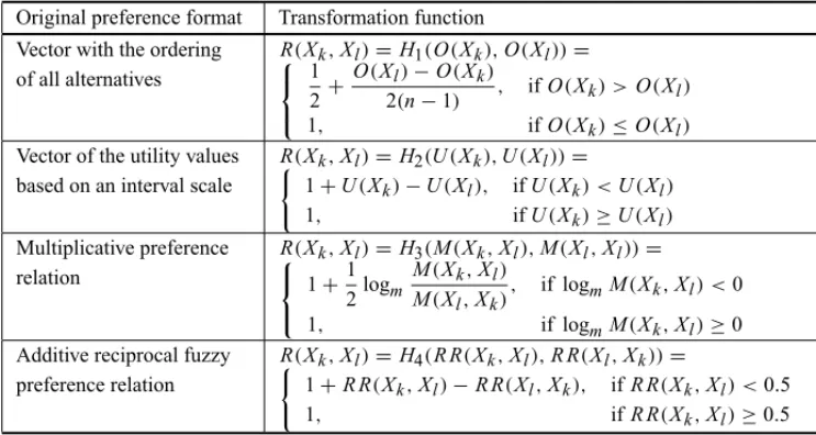
Table 1– Transformation functions for the conversion of preference information expressed in different formats into a NRFPR (Pedryczet al., 2011).
Original preference format Transformation function Vector with the ordering
of all alternatives
R(Xk,Xl)=H1(O(Xk),O(Xl))=
1 2+
O(Xl)−O(Xk)
2(n−1) , ifO(Xk) >O(Xl)
1, ifO(Xk)≤O(Xl)
Vector of the utility values based on an interval scale
R(Xk,Xl)=H2(U(Xk),U(Xl))=
(
1+U(Xk)−U(Xl), ifU(Xk) <U(Xl)
1, ifU(Xk)≥U(Xl)
Multiplicative preference relation
R(Xk,Xl)=H3(M(Xk,Xl),M(Xl,Xl))=
1+1
2logm
M(Xk,Xl) M(Xl,Xk)
, if logmM(Xk,Xl) <0
1, if logmM(Xk,Xl)≥0
Additive reciprocal fuzzy preference relation
R(Xk,Xl)=H4(R R(Xk,Xl),R R(Xl,Xk))=
(
1+R R(Xk,Xl)−R R(Xl,Xk), ifR R(Xk,Xl) <0.5
1, ifR R(Xk,Xl)≥0.5
In this paper, those transformation functions summarized in Table 1 are utilized to create a gen-eral framework for constructing NRFPRs on the basis of preference information which may be expressed in different formats. Given a set X of alternatives, a DM can express his/her pref-erences by ordering the alternatives from best to worst, by constructing a utility function or by performing pairwise comparisons between the alternatives to construct a multiplicative prefer-ence relation, a ARFPR or a NRFPR. At the same time, in order to increase the flexibility of such general framework, the results of (Ekel et al., 1998) are utilized to derive NRFPRs from the fuzzy estimates given by a DM to evaluate the alternatives. In this way, once a DM provides fuzzy estimatesFp(Xk),k=1,2, . . . ,nto evaluate all the alternatives for a criterionFpwhich can be measured on a numerical scale, if the essence of preference is coherent with the natu-ral order(≥)along the axis of measurable values of Fp, then the following expressions can be utilized to construct a NRFPR:
Rp(Xk,Xl)= sup fp(Xk),fp(Xl)∈Fp
fp(Xk)≥fp(Xl)
min Fp(fp(Xk)),Fp(fp(Xl)), (11)
Rp(Xl,Xk)= sup fp(Xk),fp(Xl)∈Fp
fp(Xl)≥fp(Xk)
min Fp(fp(Xk)),Fp(fp(Xl)), (12)
where fp(Xk)and fp(Xl)are real numbers reflecting the evaluation of the attribute Fp(with a
maximization character) for the alternatives XkandXl; Fp(fp(Xk))andFp(fp(Xl))represent
the membership functions of the fuzzy setsFp(Xk)andFp(Xl)evaluated at fp(Xk)and fp(Xl),
5 CONSTRUCTION OF NONRECIPROCAL FUZZY PREFERENCE RELATIONS WITH THE USE OF PREFERENCE FUNCTIONS
The results of (Brans & Vincke, 1985) permit one to apply preference functions as an additional format that can be used by a DM to express his/her preferences. In particular, in the family of PROMETHEE methods, the preferences being restricted to a single criterion Fp, are modeled through a preference functionsp(Xk,Xl), in such a way that it reflects the preference level ofXk
overXl, according to the following rules:
• ifsp(Xk,Xl)=0, both alternatives are considered indifferent to each other;
• ifsp(Xk,Xl)=1,Xk is strictly preferred toXl;
• if 0<sp(Xk,Xl) <1,Xkis weakly preferred toXl.
The preference functions are usually defined in terms of the difference
dp(Xk,Xl)= fp(Xk)− fp(Xl) (13)
in such a way that they transform the difference in the evaluations of two alternatives into a preference intensity between 0 and 1. The preference functions can have different shapes, as long as they are nondecreasing functions of the differencedp(Xk,Xl)(Brans & Vincke, 1985).
The methods PROMETHEE I and PROMETHEE II admit six different generalized models for the preference function, which cover most part of the scenarios encountered in real applications (Brans & Vincke, 1985). They are: the usual criterion, the quasi-criterion, the level-criterion, the linear criterion, the linear criterion with indifference region, and the Gaussian criterion. With the availability of those generalized functions, it may be easier for a DM to define a preference function reflecting his/her preferences. Next, we describe how one can construct NRFPRs based on each one of those preference functions. It should be indicated that, here we consider the criteria as being of maximization type (without loss of generality).
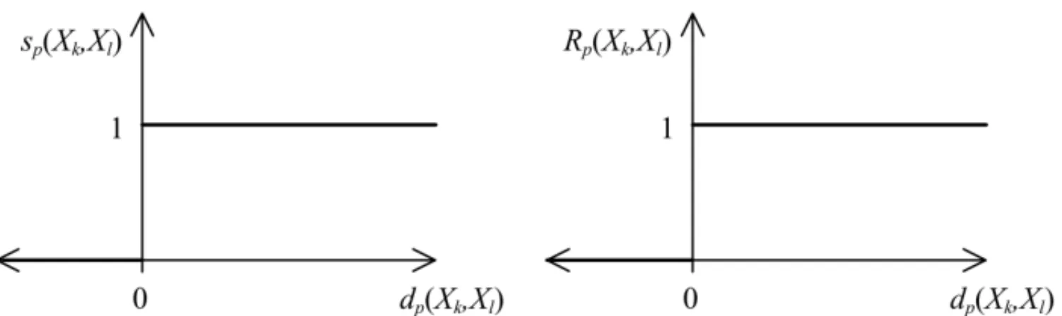
Let us begin by considering three preference functions that are particularly easy to define: the usual criterion, the quasi-criterion, and the level-criterion. Figure 1 shows the graphical represen-tation of the usual criterion, which may be considered as being the simplest type of preference function, since it does not require any parameter to be set by a DM. As it can be seen in Fig-ure 1, the level of strict preference ofXkoverXl is equal to 1 fordp(Xk,Xl) >0 and is null for dp(Xk,Xl) <0. If a DM wants to construct a NRFPR based on the usual criterion, the following
rules must be applied to the comparison of each pair of alternatives:
• ifdp(Xk,Xl) <0, thenRp(Xk,Xl)=0 andRp(Xl,Xk)=1;
• ifdp(Xk,Xl)=0, thenRp(Xk,Xl)=1 andRp(Xl,Xk)=1;
. Left side: Preference function based on the usual criterion; Right side: NRFP
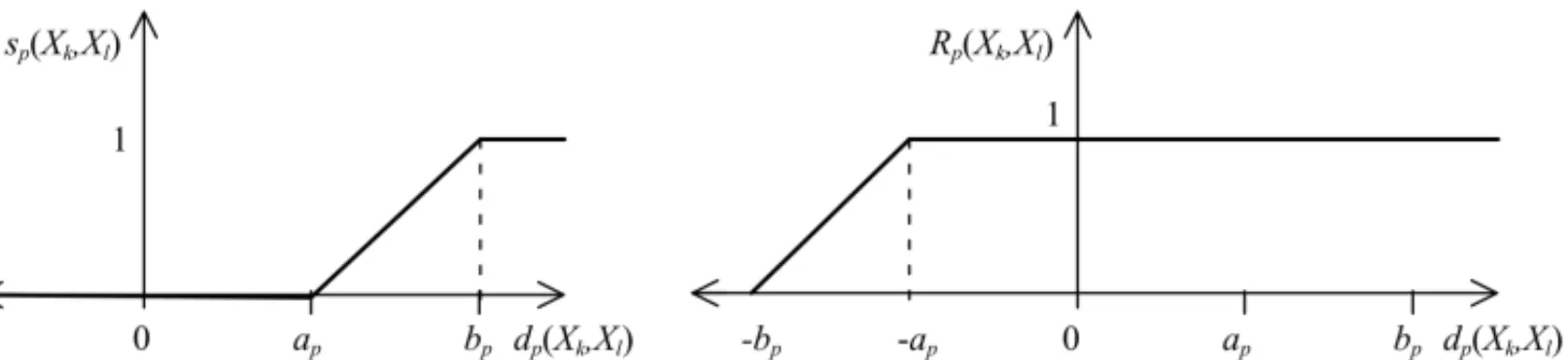
Figure 1– Left side: Preference function based on the usual criterion; Right side: NRFPR based on the usual criterion, expressed in function of the differencedp(Xk,Xl).Figure 2 shows a graphical representation of the preference function corresponding to the quasi-criterion and of the NRFPR based on the quasi-quasi-criterion. It is worth noting that the usual quasi-criterion can be seen as a particular case of the quasi-criterion where the bounds of the indifference interval
[−ap,ap]are null, that is ap =0. If a DM wants to construct a NRFPR coherently with the
quasi-criterion, the pairwise comparisons must attain the following conditions:
• ifdp(Xk,Xl) <−ap, then Rp(Xk,Xl)=0 andRp(Xl,Xk)=1;
• if−ap≤dp(Xk,Xl)≤ap, thenRp(Xk,Xl)=1 andRp(Xl,Xk)=1;
• ifdp(Xk,Xl) >ap, thenRp(Xk,Xl)=1 andRp(Xl,Xk)=0.
. Left side: Preference function based on the quasi-criterion; Right side: NRFPR
Figure 2– Left side: Preference function based on the quasi-criterion; Right side: NRFPR based on the quasi-criterion, expressed in function of the differencedp(Xk,Xl).The level-criterion allows discriminating an indifference interval[−ap,ap]and a weak
prefer-ence interval[ap,bp](and[−bp,−ap]). The pairwise comparisons must satisfy the following
conditions in order to construct a NRFPR coherently with the level-criterion:
• ifdp(Xk,Xl)≤ −bp, thenRp(Xk,Xl)=0 andRp(Xl,Xk)=1;
• if−bp<dp(Xk,Xl)≤ −ap, thenRp(Xk,Xl)=0.5 andRp(Xl,Xk)=1;
• if−ap<dp(Xk,Xl) <ap, thenRp(Xk,Xl)=1 andRp(Xl,Xk)=1;
• ifap<dp(Xk,Xl) <bp, thenRp(Xk,Xl)=1 andRp(Xl,Xk)=0.5;
Left side: Preference function based on the level criterion; Right side: NRFPR based Figure 3– Left side: Preference function based on the level criterion; Right side: NRFPR based on the level criterion, expressed in function of the differencedp(Xk,Xl).
The preference functions of the linear criterion, the linear criterion with an indifference region, and the Gaussian criterion present a smooth transition between indifference and strict preference, which permits a DM to make judgments at different levels of weak preference. The graphical representations of those preference functions are shown in the Figures 4, 5, and 6, respectively.
In the visualization of the linear criterion (refer to Fig. 4), the slope of the preference function depend on the value of the preference thresholdbp. Thus, in order to define a NRFPR coherently
with the linear criterion, the pairwise comparisons must be in accordance with the following conditions:
• ifdp(Xk,Xl) <−bp, thenRp(Xk,Xl)=0 andRp(Xl,Xk)=1;
• if−bp≤dp(Xk,Xl) <0, thenRp(Xk,Xl)=1− |dp(Xk,Xl)|/bpandRp(Xl,Xk)=1;
• if 0≤dp(Xk,Xl) <−bp, thenRp(Xk,Xl)=1 andRp(Xl,Xk)=1− |dp(Xk,Xl)|/bp;
• ifdp(Xk,Xl) >bp, thenRp(Xk,Xl)=1 andRp(Xl,Xk)=0.
Left side: Preference function based on the linear criterion; Right side: NRFP
Figure 4– Left side: Preference function based on the linear criterion; Right side: NRFPR based on the linear criterion, expressed in function of the differencedp(Xk,Xl).The Linear criterion with indifference region can be considered an extension of the linear crite-rion to deal with judgments of indifference when the pair of alternatives have similar evaluations and their difference lies in an indifference interval[−ap,ap]. A NRFPR is coherent with this
• ifdp(Xk,Xl) <−bp, then Rp(Xk,Xl)=0 andRp(Xl,Xk)=1;
• if −bp ≤ dp(Xk,Xl) < −ap, then Rp(Xk,Xl) = 1 − |dp(Xk,Xl)|/bp and Rp(Xl,Xk)=1;
• if−ap≤dp(Xk,Xl)≤ap, thenRp(Xk,Xl)=1 andRp(Xl,Xk)=1;
• ifap<dp(Xk,Xl)≤bp, thenRp(Xk,Xl)=1 andRp(Xl,Xk)=1− |dp(Xk,Xl)|/bp;
• ifdp(Xk,Xl) >bp, thenRp(Xk,Xl)=1 andRp(Xl,Xk)=0.
Left side: Preference function based on the linear criterion with indifference region; Figure 5– Left side: Preference function based on the linear criterion with indifference region; Right side: NRFPR based on the linear criterion with indifference region, expressed in function of the difference
dp(Xk,Xl).
Finally, in the case of the Gaussian criterion,σpis the distance between the origin and the
inflex-ion point of the curvesp(Xk,Xl). The Gaussian Criterion allows a transition (without
discon-tinuities) between judgments of indifference and strict preference. In order to define a NRFPR coherently with the Gaussian criterion, the pairwise comparisons must be in accordance with the following conditions:
• ifdp(Xk,Xl) <0, thenRp(Xk,Xl)=exp(−|dp(Xk,Xl)|/2σp2)andRp(Xl,Xk)=1;
• ifdp(Xk,Xl)≥0, thenRp(Xk,Xl)=1 andRp(Xl,Xk)=exp(−|dp(Xk,Xl)|/2σp2),
whereσpis the distance between the origin and the inflexion point of the preference function.
Left side: Preference function based on the Gaussian criterion; Right side: NRF
It is not difficult to demonstrate that NRFPRs constructed coherently with those six types of pref-erence functions always satisfy weak transitivity (refer to expression (9)). For this demonstration, it is worth noting thatRp(Xk,Xl)≥ Rp(Xl,Xk)only ifsp(Xk,Xl)≥0 (which the reader can
easily verify for each type of preference function) and that a nondecreasing preference function satisfiessp(Xk,Xl) ≥ 0 only if dp(Xk,Xl) ≥ 0. In this way, if Rp(Xk,Xj) ≥ Rp(Xj,Xk)
andRp(Xj,Xl) ≥ Rp(Xl,Xj), thendp(Xk,Xj) ≥ 0 (which means that fp(Xk) > fp(Xj))
and, at the same time,dp(Xj,Xl)≥0 (which means that fp(Xj) > fp(Xl)). It is also possible
to infer that fp(Xk) > fp(Xj) > fp(Xl), which results indp(Xk,Xl)≥ 0,sp(Xk,Xl)≥ 0,
andRp(Xk,Xl) > Rp(Xl,Xk).
6 A METHOD FOR MULTICRITERIA DECISION MAKING BASED ON THE
ORLOVSKY CHOICE PROCEDURE
The Orlovsky choice procedure makes use of a fuzzy strict preference relation given by (7) to carry out the choice of alternatives (Orlovsky, 1978, 1981). Considering the pth criterion, as
Pp(Xl,Xk)describes the set of all alternatives Xkthat are strictly dominated by Xl, its compli-mentPp(Xl,Xk)corresponds to the set of alternatives that are not dominated by Xl. Therefore, in order to meet the set of alternatives fromX that are not dominated by any other alternative, it suffices to obtain for each alternativeXkbelonging toXthe intersection ofPp(Xl,Xk)for allXl
belonging to X. This intersection is the set of nondominated alternatives with the membership function
N Dp(Xk)= inf
Xl∈X
{1−Pp(Xl,Xk)} =1− sup Xl∈X
Pp(Xl,Xk) , (14)
which reflects the level of nondominance of each alternativeXk.
A natural choice for a monocriteria problem based on this model should be the alternatives providing:
XN DRp =
n
XkN D∈ X|RN Dp (XkN D)= sup Xk∈X
N Dp(Xk)o. (15)
It is worth emphasizing that the alternatives satisfying
XRN Dp =
n
XkN D∈ X|RN Dp (XkN D)=1
o
(16)
are actually nonfuzzy nondominated and can be considered as the nonfuzzy solution for the choice problem (Orlovsky, 1978, 1981).
Expressions (7), (14), and (15) may be used to solve choice or ranking problems not only with a single criterion, but also with multiple criteria. In particular, several procedures that allow one to include multiple criteria in the analysis of a decision making problem are discussed in Orlovsky (1981), Ekel & Schuffner Neto (2006). Let us consider one of them.
Having at hand nonstrict preference relations for each criterion, one possible procedure for solv-ing multicriteria problems consists in obtainsolv-ing a global relation through the intersection of those relations as follows:
The use of intersection to aggregate all criteria is suitable, when it is a necessary condition that a good alternative Xkmust simultaneously satisfyF1andF2and. . .andFq. Among thet-norm operators, the use of the min operator, as proposed in (Orlovsky, 1981), allows one to construct the global fuzzy nonstrict preference relation
G(Xk,Xl)=min
R1(Xk,Xl), . . . ,Rq(Xk,Xl) (18)
under a completely non-compensatory approach for multicriteria decision-making, in the sense that the high satisfaction of some criteria does not relieve the remaining ones from the require-ment of being satisfied (there is no compensation among the criteria). Such approach is also considered pessimistic, since it gives emphasis to the worst evaluations of each alternative.
Having at hand the global fuzzy nonstrict preference relation, equations (7), (14) and (15) can be subsequently applied directly toGand the result corresponds to a fuzzy set of nondominated alternatives fulfilling the role of a Pareto set (Orlovsky, 1981).
However, in case of not being possible to distinguish two or more alternatives, the contraction of (18) is possible by differentiating the importance of Rp, p = 1, . . . ,q with the use of the weighted sum:
T(Xk,Xl)= q
X
p=1
λpRp(Xk,Xl) , (19)
whereλp, p = 1, . . . ,q are importance factors of the corresponding criteria, defined aswp ∈ [0,1]andPq
p=1wp=1.
The construction of T(Xk,Xl), allows one to obtain the membership function N DT(Xk)of the fuzzy set of nondominated alternatives by subsequently applying (7) and (14) to (19). The intersection
Q(Xk)=min N D(Xk),N DT(Xk), (20)
provides us with a set of alternatives with the highest level of nondominance
XN D =
XkN D|XkN D ∈X, Q(XkN D)= sup
Xk∈K
Q(Xk)
. (21)
7 APPLICATION EXAMPLE
The multicriteria decision-making problem related to the site selection for constructing a new hospital is studied in Vahidnia et al. (2009). Here, we consider a simplified version of this problem, in which six sites are to be ranked, taking into account the following four criteria:
1. Distance from the arterial routes (minimization criterion);
2. Land cost (minimization criterion);
3. Population density (maximization criterion);
Hospitals should be located close to main public transport routes. Here, criterionF1allows one to evaluate the distance from each site to the closest arterial route. Besides, for social convenience, it is important to guarantee that every person lives in an area with accessible hospital service. CriterionF4evaluates the average time one would take to travel between the site and the nearest existing hospital. The fifth criterion which could be considered is associated with the pollution level present at each site. However, as the sites considered here do not significantly differ with respect to this criterion, the DM decided to eliminate it from the subsequent multicriteria anal-ysis. Figure 7 presents the fuzzy scores utilized for evaluating the third criterion,F3-population density. Table 2 shows the evaluation matrix of the alternatives.
Figure 7– Valuation of criterionF3(population density).
Table 2– Evaluation matrix of the alternatives.
F1(Xk) F2(Xk)
F3(Xk)
F4(Xk)
(m) ($/m2) (minutes)
X1 0 28 middle 22
X2 350 24 high 17
X3 150 18 high 12
X4 500 15 middle 10
X5 50 8 low 7
X6 300 10 very high 5
When the criterion F1 was considered by the DM, he decided not to infer the degrees of his preferences directly from those distances listed in Table 2. The DM felt more comfortable with utilizing the multiplicative preference relation to articulate his preferences as follows:
M1=
1 4 4 4 3 4
1/4 1 1/3 3 4 1 1/4 3 1 4 1/3 1/2 1/4 1/3 1/4 1 1/4 1/2 1/3 1/4 3 4 1 4 1/4 1 2 2 1/4 1
. (22)
times larger than the distance of X5,X5is not considered ten times better thanX4. At the same time, the distance of X2is higher than the distance ofX6. However, the DM judgedX2andX6 as being indifferent to each other. Besides, it is important to indicate that although (22) does not satisfy the multiplicative transitivity, the NRFPR
R1=
1 1 1 1 1 1
0.226 1 0.333 1 1 1 0.226 1 1 1 0.333 0.52 0.226 0.333 0.226 1 0.226 0.52 0.333 0.226 1 1 1 1 0.226 1 1 1 0.307 1
(23)
constructed with the use of H3 (refer to Table 1) satisfies the weak transitivity and this is a satisfactory level of consistency for the application of the decision-making method to be used.
In the case of criterionF2, the DM decided to use a preference function corresponding to a Linear criterion withb2=5($/m2). The obtained NRFPR is as follows:
R2=
1 0.2 1 1 1 1 1 1 1 1 1 1 1 1 1 0.4 1 1 1 1 1 1 1 1 1 1 1 1 1 1 1 1 1 1 1 1
. (24)
The population density of each alternative, which is related to criterionF3, was estimated by him, by the linguistic terms shown in Table 2. By applying the expressions (11) and (12) to construct a NRFPR from the comparison of fuzzy estimates, the following NRFPR is obtained:
R3=
1 0.5 0.5 1 1 0 1 1 1 1 1 0.5 1 1 1 1 1 0.5 1 0.5 0.5 1 1 0 0.5 0 0 0.5 1 0
1 1 1 1 1 1
. (25)
Finally, in the case of criterionF4, a preference relation corresponding to a Quasi-criterion, with
a4=3 min. The obtained NRFPR is as follows:
R4=
1 1 1 1 1 1 0 1 1 1 1 1 0 0 1 1 1 1 0 0 1 1 1 1 0 0 0 1 1 1 0 0 0 0 1 1
Having at hand the NRFPRs (23)-(26), the multicriteria analysis begins by applying (18) to obtain a global relation under a pessimistic approach through the intersection:
G=
1 0.2 0 1 0 0
0 1 0 1 0 0
0 0 1 0.4 0 0
0 0 0.226 1 0 0
0 0 0 0.5 0 0
0 0 0 0 0.307 0
. (27)
Afterward, expression (7) provides the strict preference relation
P=
0 0.2 0 1 0 0
0 0 0 1 0 0
0 0 0 0.174 0 0
0 0 0 0 0 0
0 0 0 0.5 0 0
0 0 0 0 0.307 0
. (28)
Finally, with the use of (14), we obtain the nondominance degrees of each alternative
N D=1 0.8 1 0 0.693 1
. (29)
We can order them from best to worst as(X1 ≈ X3 ≈ X6) ≻ X2 ≻ X5 ≻ X4. In order to distinguish alternatives X1, X3, and X6, a subsequent analysis is performed by applying (19) and (20). Considering that the DM defined the weights of the criteria asλ1 = λ2 = 0.2 and λ3=λ4=0.3, the convolution (19) provides the following matrix of pairwise comparisons:
T =
1 00.69 0.65 0.8 0.8 0.55 0.545 1 0.667 0.8 0.8 0.65 0.545 0.7 1 0.88 0.667 0.554 0.545 0.417 0.695 1 0.645 0.404 0.417 0.245 0.4 0.85 1 0.7 0.545 0.7 0.7 0.7 0.781 1
. (30)
In this way, by processing (30) with the use of (7) and (14), it is possible to obtain the following fuzzy set of nondominated alternatives:
N DT =
0.95 0.855 0.854 0.617 0.445 1
. (31)
Finally, the intersection of (29) and (30), obtained in accordance with (20), makes it possible to contract the fuzzy set of nondominated alternatives as follows:
N D=0.95 0.8 0.854 0 0.445 1
. (32)
The final ranking of the alternatives can be defined on the basis of (32) as
CONCLUSIONS
In this paper we showed how the preference functions can be utilized to construct NRFPRs. The preference functions correspond to a well established preference format which has been utilized to model the preferences of a DM in the methods PROMETHEE I and PROMETHEE II. The results of this paper allow a more flexible input of preferences in the decision-making process based on the analysis ofhX,Rimodels (now, it is possible to offer to a DM the following formats: the ordering of the alternatives, the utility values, the multiplicative preference relations, the fuzzy estimates, the reciprocal as well as the nonreciprocal fuzzy preference relations and the preference functions). The applicability of the proposed procedure is demonstrated through the solution of a multicriteria decision-making problem related to the site selection for constructing a new hospital.
ACKNOWLEDGMENTS
This research is supported by the National Council for Scientific and Technological Development of Brazil (CNPq) – grants PQ: 307406/2008-3 and PQ: 307474/2008-9.
REFERENCES
[1] ALSINAC. 1985. On a family of connectives for fuzzy sets.Fuzzy Sets and Systems,16: 231–235. [2] BELTONV. 1999. Multiple-criteria problem structuring and analysis in a value theory framework.
In:Multicriteria decision making: advances in MCDM models, algorithms, theory[edited by GALT, STEWARTT & HANNET], Kluwer Academic Publishers, Dordrecht, 12-2-12-29.
[3] BRANSJP & VINCKE PH. 1985. A preference ranking organization method (the PROMETHEE method for multiple criteria decision-making.Management Science,31: 647–656.
[4] DEBAETSB & FODORJC. 1997. Twenty years of fuzzy preference structures.Rivista di Matematica per le Scienze Economiche e Sociali,20: 45–66.
[5] CHICLANAF, HERRERAF & HERRERA-VIEDMAE. 1998. Integrating three representation models in fuzzy multipurpose decision making based on fuzzy preference relations.Fuzzy Sets and Systems, 97: 33–48.
[6] CHICLANAF, HERRERA F & HERRERA-VIEDMAE. 2001. Integrating multiplicative preference relations rain a multipurpose decision-making model based on fuzzy preference relations.Fuzzy Sets and Systems,122: 277–291.
[7] EKELP, PEDRYCZW & SCHINZINGERR. 1998. A general approach to solving a wide class of fuzzy optimization problems.Fuzzy Sets and Systems,97: 49–66.
[8] EKELP.YA. & SCHUFFNERNETOFH. 2006. Algorithms of discrete optimization and their applica-tion to problems with fuzzy coefficients.Information Sciences,176: 2846–2868.
[9] FARQUHARPH & KELLERLR. 1989. Preference intensity measurement.Annals of Operations Re-search,19: 205–217.
[11] FODORJC & ROUBENSM. 1994b. Valued preference structures.European Journal of Operational Research,79: 277–286.
[12] HERRERA-VIEDMAE, HERRERAF & CHICLANA F. 2002. A consensus model for multiperson decision making with different preference structures.IEEE Transactions on Systems, Man and Cy-bernetics – Part A: Systems and Humans,32: 394–402.
[13] HERRERA-VIEDMAE, HERRERAF, CHICLANAF & LUQUEM. 2004. Some issues on consistency of fuzzy preference relations.European Journal of Operational Research,154: 98–109.
[14] KULSHRESHTHAP & SHEKARB. 2000. Interrelations among fuzzy preference-based choice func-tions and significance of rationality condifunc-tions: A taxonomic and intuitive perspective.Fuzzy Sets and Systems,109: 429–425.
[15] LUJ, ZHANGG, RUAND & WUF. 2007.Multi-objective Group Decision Making: Methods, Soft-ware and Applications with Fuzzy Set Techniques.Imperial College Press, London.
[16] ORLOVSKYSA. 1978. Decision-making with a fuzzy preference relation.Fuzzy Sets and Systems,1: 155–167.
[17] ORLOVSKYSA. 1981.Problems of Decision Making with Fuzzy Information(in Russian), Nauka, Moscow.
[18] PEDRYCZW, EKELP & PARREIRASR. 2011.Fuzzy Multicriteria Decision-Making: Models, Meth-ods, and Applications.Wiley, Chichester.
[19] QUEIROZJCB. 2009. Models and Methods of Decision Making Support for Strategic Management: PhD thesis (in Portuguese), Federal University of Minas Gerais, Belo Horizonte.
[20] SAATYT. 1980. The Analytic Hierarchy Process. McGraw Hill, New York.
[21] SENGUPTAK. 1998. Fuzzy preference and Orlovsky choice procedure.Fuzzy Sets and Systems,93: 231–234.
[22] VAHIDNIAMH, ALESHEIKHAA & ALIMOHAMMADIA. 2009. Hospital site selection using fuzzy AHP and its derivatives.Journal of Environmental Management,90: 3048–3056.
[23] WANG X. 1997. An investigation into relations between some transitivity-related concepts.Fuzzy Sets and Systems,89: 257–262.