www.ann-geophys.net/29/1331/2011/ doi:10.5194/angeo-29-1331-2011
© Author(s) 2011. CC Attribution 3.0 License.
Annales
Geophysicae
The correlation between solar and geomagnetic activity – Part 1:
Two-term decomposition of geomagnetic activity
Z. L. Du
Key Laboratory of Solar Activity, National Astronomical Observatories, Chinese Academy of Sciences, Beijing 100012, China
Received: 30 November 2010 – Revised: 29 May 2011 – Accepted: 17 July 2011 – Published: 5 August 2011
Abstract.By analyzing the logarithmic relationship between geomagnetic activity as represented by the annualaaindex and solar magnetic field activity as represented by the an-nual sunspot number (Rz) during the period 1844–2010,aa is shown to lie in between two lines defined solely byRz. Two ways can be used to decompose theaaindex into two components. One is decomposing aa into the sum of the baseline (aab) and the remainder (aau) with a null corre-lation. Another is dividing the top-line (aat) into the sum ofaaand the remainder (aad) with a null correlation. The first decomposition is similar to the traditional one. The second decomposition implies a nonlinear relationship of aa with Rz (aat) and a decay process (aad). Therefore, aat=aa+aad=aab+aau+aad: (i) aat is related to the solar energy potential of generating geomagnetic activity (as-sociated withRz); (ii)aabis related to transient phenomena; (iii)aauis related to recurrent phenomena; and (iv)aadis re-lated to the energy loss in the transmission from solar surface to the magnetosphere and ionosphere that failed to generate geomagnetic activity.
Keywords. Magnetospheric physics (Solar wind-magnetosphere interactions)
1 Introduction
Since Mayaud (1972) designed the geomagnetic activityaa index from the 3-hourly K indices at two near-antipodal mid-latitude stations, numerous authors have used it to analyze the global geomagnetic activity and its correlation with so-lar activity (Schatten et al., 1978; Feynman, 1982; Legrand and Simon, 1989a; Nevanlinna and Kataja, 1993; Lukianova
Correspondence to:Z. L. Du ([email protected])
et al., 2009; Du et al., 2009; Du, 2011a). Theaaindex ap-pears an 11-year cycle similar to that of sunspot activity, as described by the Zurich sunspot number (Rz). Studying the relationship between geomagnetic activity, as represented by aa, and solar activity, as represented byRz, may contribute to understanding the origin and formation of the former.
Geomagnetic activities have long been known to be cor-related with solar activities (Snyder et al., 1963; Russell and McPherron, 1973; Garrett et al., 1974; Feynman and Crooker, 1978). Geomagnetic activities can be resulted from variable current systems formed in the magnetosphere and ionosphere, such as the ring current and auroral ionospheric current, which are strongly modulated by solar activities via the interaction of the magnetosphere with solar winds (Feyn-man, 1980; Legrand and Simon, 1989a,b; Demetrescu and Dobrica, 2008) or others (Legrand and Simon, 1981, 1989a; Stamper et al., 1999; Tsurutani et al., 2006). It is believed that the geomagnetic activity is well associated with the so-lar wind speed (V), the southward component (Bz) of the interplanetary magnetic field (IMF) and their product (Sny-der et al., 1963; Russell and McPherron, 1973; Garrett et al., 1974; Crooker et al., 1977; Svalgaard, 1977; Feynman, 1980; Wang and Sheeley, 2009). In general, the magnetosphere exhibits approximately a linear response to the solar wind drivers. However, a nonlinear behavior is significant in the declining phase of a solar cycle, which is related to increased solar wind speeds (Legrand and Simon, 1989a,b; Venkatesan et al., 1991; Echer et al., 2004; Johnson and Wing, 2005).
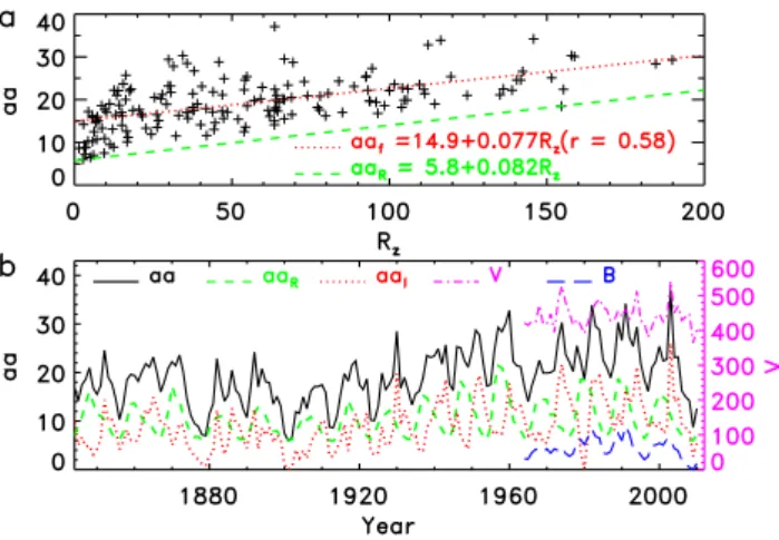
Fig. 1. (a)Scatter plot ofaaagainstRz(pluses), linear fit (dotted), and baselineaaR(dashed). (b)The time series ofaa(solid),aaR
(dashed) from Eq. (2) andaaI(dotted) from Eq. (3) since 1844. The
time series ofV (dash-dotted) andB(long-dashed) since 1964 are also shown for comparison, with theBvalues so scaled that they can be clearly seen.
the declining phase or at the solar minimum of the cycle (Legrand and Simon, 1981; Venkatesan et al., 1982; Legrand and Simon, 1989a,b; Tsurutani et al., 2006). Feynman (1982) analyzed the relationship between the annualaaandRz se-ries from 1869 to 1975 and found that theaavalues are all above a base line (aaR) that is linearly related toRz. Then, she decomposed theaa index into two equally strong peri-odic components: aaR and the remainder aaI=aa−aaR. The first one (the “short lived” R component) is associated with the transient phenomena and follows the sunspot cycle, while the second one (the “slowly varying” interplanetary I component) is associated with the recurrent phenomena and is almost 180◦out of phase with the sunspot cycle (Hathaway and Wilson, 2006). Legrand and Simon (1989a) classified the geomagnetic activity in four classes: the magnetic quiet ac-tivity, the recurrent acac-tivity, the fluctuating acac-tivity, and the shock activity. At mid-latitude, the geomagnetic activity is sensitive both to the auroral phenomena (particle precipita-tions, substorms, and auroras) which are at the origin of the auroral electrojet (AE) activity, and to the equatorial ring cur-rent which is the source of the geomagnetic storms (Legrand and Simon, 1989a,b). Therefore, theaaindex is an integral effect of various sources of geomagnetic activity.
The relationship between the solar and geomagnetic activ-ity is not a simple linear one (Feynman, 1983; Legrand and Simon, 1983) due to various sources of geomagnetic activ-ity. Decomposing the geomagnetic activity (aaindex) into different parts may help understand its origins.
In this paper, we first reexamine the work of Feynman (1982) to decompose the annualaaindex for the data avail-able (Sect. 2) into two components based on a linear relation-ship betweenaaandRz(Sect. 3). To elucidate howaa de-pends onRz, we analyze the scatter plot oflnaaagainstlnRz
in Sect. 4. All the data points are found to be in between the two lines of baseline (lnaab) and top-line (lnaat). Accord-ing to the baseline, theaaindex can be decomposed into two components: aaband the remainderaau=aa−aabwith a null correlation (Sect. 4.1). This decomposition is similar to that of Feynman (1982), but the relationship betweenaab andRz is nonlinear. The top-line provides another way to decomposeaatinto two components:aaandaad=aat−aa with a null correlation (Sect. 4.2). We attempt to explain the second decomposition by a nonlinear model (Sect. 4.2.1) and a decay process (Sect. 4.2.2). Theaaindex is the remainder ofaatafter decayaad. Some conclusions are discussed and summarized in Sect. 5.
2 Data
To suppress the high frequencies involved in the solar ro-tation and seasonal variations, in this study the geomag-netic activity is represented by the annual averages of aa index (Mayaud, 1972) using reliable values since 18681and the equivalent ones from measurements in Finland from 1844 to 1867 (Nevanlinna and Kataja, 1993). The solar (magnetic field) activity is represented by the annual averages ofRz2 from 1844 to 2010. In addition, for comparison we use the annual speed (V) and magnetic field (B) of solar wind from the OMNI data sets since 19643, and the Dst (disturbance storm time)4index representing the ring current (Gonzalez et al., 1990) since 1958.
3 Two-term decomposition ofaaaccording to the linear relationship betweenaaandRz
In this section, we repeat the Feynman (1982) work to de-composeaainto two components, using the data from 1844 to 2010. Figure 1a shows the scatter plot ofaaagainstRz (pluses). The dotted line indicates the linear fit ofaatoRz, with the regression equation given by
aa=14.9+0.077Rz. (1)
It is seen that the data points are all above the (dashed) base-line, defined by the lower envelope,
aaR=5.8+0.082Rz. (2)
The remainder ofaais then
aaI=aa−aaR. (3)
Figure 1b shows the time series ofaa(solid),aaR(dashed), andaaI(dotted) since 1844. The correlation coefficient be-tween the two components, aaR and aaI, is almost zero
1ftp://ftp.ngdc.noaa.gov/STP/SOLAR DATA/RELATED
INDICES/AA INDEX/
2http://www.ngdc.noaa.gov/stp/spaceweather.html
Table 1.Correlation coefficients (r) betweenaa,Rz,aaR,aaI,V,
andB.
r aa aaR(Rz) aaI V B
aa 1 0.58 0.79 0.74 0.83
aaR(Rz) 1 −0.05 −0.06 0.78
aaI 1 0.84 0.31
V 1 0.32
(r= −0.05), implying thataaIhas a 90◦(∼3-yr) rather than a 180◦ (Feynman, 1982; Li, 1997; Hathaway and Wilson, 2006) phase shift toaaR. The phase shift is related to the time delay ofaatoRz(Echer et al., 2004; Du, 2011b). Fig-ure 1b also showsV (dash-dotted) andB(long-dashed) since 1964 for comparison. The correlation coefficients between these parameters are listed in Table 1.
One sees in Table 1 that: (i)aais positively correlated with Rz(r=0.58),aaR(r=0.58),aaI(r=0.79),V (r=0.74), and B (r=0.83); (ii) aaR(Rz) is well correlated with B (r=0.78) but has a null correlation withV (r= −0.06); and (iii)aaIhas a much higher correlation withV (r=0.84) than withB (r=0.31). Therefore,aaRandaaIare well associ-ated withBandV, respectively.
The two components ofaaRandaaIhave been explained by two main solar sources of geomagnetic activity (Legrand and Simon, 1981; Venkatesan et al., 1982; Legrand and Si-mon, 1989a; Gonzalez et al., 1990; Venkatesan et al., 1991; Legrand and Simon, 1989a,b; Echer et al., 2004): (i)aaR is related to solar flares and coronal mass ejections (CMEs); and (ii)aaIis related to high-speed solar wind streams and is out of phase with the sunspot cycle (Feynman, 1982).
4 Two-term decomposition ofaaaccording to the loga-rithmic relationship betweenaaandRz
To elucidate howaadepends onRz, we analyze the corre-lation between thenatural logarithmsof the annualaaand Rzfrom 1844 to 2010. The scatter plot oflnaaagainstlnRz is shown in Fig. 2. The dotted line indicates the linear fit of
lnaatolnRz, with the regression equation given by
lnaa=2.13+0.21lnRz, or aa=8.41Rz0.21. (4) The positive correlation betweenlnaaandlnRz(r=0.67) is stronger than that betweenaa andRz (r=0.58), implying thataa varies preferably nonlinearly withRz. Also shown in the figure are the years of the maximum (triangles) and minimum (circles) amplitudes of the sunspot cycle.
One very prominent property in Fig. 2 is that the data points are all in between the two parallel (dashed) lines with
Fig. 2. Scatter plot oflnaa againstlnRz(black pluses for odd-numbered cycles and purple crosses for even-odd-numbered cycles) with a correlation coefficient ofr=0.67. The dotted line indicates the linear fit oflnaa tolnRz. The data points are all in between the
two parallel (dashed) lines oflnaat(top) andlnaab(base).
Trian-gles and circles denote the years of the maximum and minimum amplitudes of the sunspot cycle, respectively. The coordinate axisη
describes decay strength.
their equations defined (from two points on baseline or top-line) by
lnaab=1.36+0.29lnRz, or aab=e1.36Rz2/7 (5) and
lnaat=2.44+0.29lnRz, or aat=e2.44R2z/7. (6) The above equations suggest that a certain level of solar ac-tivity (Rz) is associated with at least (most)aab(aat) of the geomagnetic activity. Fromaabandaat, two new indices, aauandaad, can be defined such that
aa=aab+aau, or aau=aa−aab (7) and
aat=aa+aad, or aad=aat−aa. (8) The null correlation ofaabwithaau(r=0.09) implies that aa can be decomposed into two independent components: aabandaau. Similarly, the null correlation ofaawithaad (r= −0.0003) implies thataatcan be divided into two inde-pendent orthogonal terms:aaandaad.
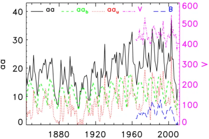
Fig. 3. Time series ofaa(solid),aab(dashed) from Eq. (5),aau
(dotted) from Eq. (7),V (dash-dotted), andB(long-dashed), with theBvalues so scaled that can be clearly seen.
withaat(r=0.62), Therefore, some underlying information must exist in bothaauandaad.
The strong correlation ofaadwithRz (r=0.75) and the null correlation ofaadwithaa(r=0.00) imply thataadis well associated with the level ofRz (solar activity). In con-trast, the strong correlation of aau withaa (r=0.84) and the null correlation ofaauwithRz(r=0.07) imply thataau reflects the variation inaa(geomagnetic activity).
4.1 Two-term decomposition ofaabased on the baseline
Similar to Sect. 3, one decomposition method of theaa in-dex is according to the baseline (aab), as theaavalues are all aboveaab(Fig. 2). Figure 3 shows the two components, aab(dashed) from Eq. (5) andaau(dotted) from Eq. (7), to-gether withaa(solid),V (dash-dotted), andB(long-dashed) for comparison. The correlation coefficients between these parameters are listed in Table 2.
The following may by noted in Table 2: (i) aa is posi-tively correlated withaab,aau, V, andB; (ii)aab is well correlated withB (r=0.83) but has a null correlation with V (r=0.03); and (iii)aauhas a much higher correlation with V (r=0.85) than withB(r=0.41). Therefore,aabandaau are well associated withBandV, respectively, reflecting the two sources of geomagnetic activity.
This decomposition is similar to that in Sect. 3. Theaab andaauterms in this section correspond similarly to the R and I components in the previous section, respectively. The main discrepancy is that the R component is linearly related toRz (Eq. 2), whileaab is related toRz in the form of a power-law (Eq. 5). Thus, the aab component can be ex-plained to be nonlinearly related to solar flares and CMEs, and theaau component is related to high-speed solar wind streams having a 90◦(∼3-yr) phase shift toaab.
It should be pointed out in Fig. 2 that there is a maxi-mum (aat) for the aavalues and that there is a maximum
Table 2.Correlation coefficients betweenaa,aab,aau,V andB.
r aa aab aau V B
aa 1 0.62 0.84 0.74 0.83
aab 1 0.10 0.03 0.83
aau 1 0.85 0.41
(aat−aab) for theaaucomponent, which is part ofaaabove the baselineaab(Eq. 7). This result suggests thatRzis asso-ciated with a certain amount of solar energy (Et) potential of generating geomagnetic activity (aa) whose maximum (aat) is related toEt. The energy (Et) consists of three parts: (i) the first part (Eb), being related to the transient phenomena, gen-erates the geomagnetic activity (aab) that is well associated withRz(aab∝R2z/7); (ii) the second part (Eu), being related to the recurrent phenomena, generates the geomagnetic ac-tivity (aau) that is almost uncorrelated with the former (aab); and (iii) the third part (Ed=Et−Eb−Eu), generating no geomagnetic activity, might be interpreted as the energy loss in the energy transmission from solar surface to the magne-tosphere and ionosphere, which may involve very complex processes (see also Sect. 4.2 and Discussion) and may be re-lated to the time delay of geomagnetic activity (aa) to solar activity (Rz).
For the decomposition in Fig. 2, theaavalues are all above the baselineaaR(Eq. 2), while there seems to be no upper limit for theaaoraaI(Eq. 3) values shown in Fig. 1a – at least such a limit (if existing) is not apparent.
4.2 Two-term decomposition ofaabased on the top-line
Another alternate decomposition method is by use of the top-line (aat), as theaavalues are all belowaat (Fig. 2). The two components,aaandaadfrom Eqs. (6) and (8), have a null correlation (r∼0), implying that theaaindex has a 90o (∼3-yr) phase shift to aad. This decomposition might be explained by a nonlinear model and a decay process.
4.2.1 A nonlinear model
Suppose that the variation rate ofaais proportional to that ofRz,
1aa aa ∝
1Rz Rz , or
∂aa ∂Rz =γ
aa
Rz, (9)
whereγ is called “response efficiency” ofaa to Rz. The solution to this equation is in the form of
whereβ is an integral constant. Thus, Eq. (10) can be taken as a general form of Eqs. (5)–(6) for
γ =2/7, βt=2.44, βb=1.36.
(11)
It suggests from Eqs. (10) and (4) that aa varies with Rz nonlinearly rather than linearly. In fact, the values ofγ for the top- and base-line are not strictly equal to one another. By carefully examining the top-line in Fig. 2, two possible values ofγ areγt=0.27 and 0.31 (from two different pairs of the upper envelope), corresponding toβt=2.49 and 2.39, respectively. We have taken an average ofγt=0.29, which is equal toγb=0.29 for the baseline, and βt=2.44 corre-spondingly. Therefore,γ andβ have uncertainties of about 1γ=0.02 and1β=0.05, respectively. Theγ value reflects the generation efficiency ofaaby solar (activity) energy that is related toRz, only about 2/7 (29 %) of the relative vari-ation inRz being related to the variation inaa in terms of annual averages.
4.2.2 A decay process
From Eqs. (5), 6), and (11) we have
aab=e−(βt−βb)aat=e−1.08aat. (12)
In accordance with this equation, all the data points in Fig. 2 can be divided into many groups, each lying on an oblique narrow stripe (belt) parallel to the top-line. These stripes are denoted by a coordinate axis (η).
Suppose thataaundergoes a decay process in terms of the variablez,
−1aa∝aa1z, or ∂aa ∂z = −
1
Laa, (13)
whereLis the decay scale. Its solution is
aa(z)=e−z/Laa0, (14)
whereaa0is an integral constant. Because theaavalues are all in between the two lines (Fig. 2),z=0 can be taken as the top-line andaa0=aatas the boundary condition, so that aa(z)=
e−z/Laat,0≤z≤1.08L,
aab, z >1.08L, (15)
and the decay term is aad(z)=aat(z)−aa(z)
=
(1−e−z/L)aat,0≤z≤1.08L, aat−aab, z >1.08L.
(16)
The above two equations can be easily explained ifzis tem-porarily taken as a length variable with its origin at the “outer surface” of the magnetosphere and its positive direction to-wards the Earth. (i) At first, the interaction of solar activities
(solar winds and CMEs, etc.) with the magnetosphere pro-duces geomagnetic activity (aa=aat), which is the top-line in Fig. 2. Then aat undergoes a decay process according toaad(z)=(1−e−z/L)aat for 0≤z≤1.08Las it attempts to go through the decay range (ionosphere as well as mag-netosphere, hereafter DR, where aadecays). Only the re-mainderaa(z)=aat−aad(z)=e−z/Laat is observed after the DR. Various decays, due to various thicknesses and den-sities of the DR for different districts or different time peri-ods (and different solar activities), constitute the randomly scattered points of aa in Fig. 2 (the random distribution of aad or aa is the cause of the null correlation between them). (ii) Forz >1.08L,aa has already passed over the DR and will not decay further. As the maximum decay in the whole DR isaad=aat−aab, the minimumaa is then aa=aat−aad=aab, which is the baseline in Fig. 2.
It should be noted that the decay aad is well correlated withaat(r=0.78) orRz(r=0.75), meaning that a higher level of Rz tends to be associated with a larger aad or z. Although a stronger (weaker) solar activityRz (correspond-ing to the energyEt) is related to a higher (lower) level of aat, more (less) decays (or the “energy loss”Ed) will also be produced while transmitting through the DR. When aa has finally passed over the DR, only a part is left: the ob-servedaa=aat−aad(or the energyE=Et−Ed). Thus, the variablezis in fact a quantity to describe the decay strength (or the energy lossEd) in the DR, andLis the decay scale (or the maximum energy lossEd,max). Thez/L value re-flects the energy loss rate (Ed/Ed,max), which is related to the intensity and orientation of the solar dipole (Simon and Legrand, 1989), the topology and density (especially the ion density) of the DR, the size and shape of the current sheet, or the ion inertial scale (Leamon et al., 2000; Matthaeus et al., 2008). The formation is related to the interaction mech-anism of solar activities (solar winds and CMEs, etc.) with the magnetosphere (and of the fast with slow solar winds) and the state (strength, velocity, and direction) of the solar wind. More geomagnetic activities can be produced if the solar wind reaches the magnetosphere perpendicularly than in any other direction.
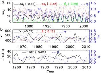
Fig. 4. (a)aad (solid) from Eq. (8),aat (dotted) from Eq. (6)
andRz(dashed) since 1844.(b)V (solid),B(dotted), andη (dash-dotted) since 1964.(c)−Dst (solid) andη(dash-dotted) since 1958. The values ofRzandBare so scaled that they can be clearly seen. The numbers in brackets indicate the correlation coefficients of the parameters withη.
asaatin Eq. (6), and the decay process can be described by Eq. (16).
4.2.3 aa’s expression and decay indexη
Combining Eq. (6) with Eq. (15), all theaa values can be mathematically expressed as
aa=e2.44−ηRz2/7 (0≤η≤1.08), (17) where
η=z/L (18)
is called “decay index”: the quantity ofznormalized to L (Fig. 2), which is related to the decay rate, aad/aat=1− e−η. Implied in Eq. (17) is that the geomagnetic activity is generated via a nonlinear relationship withRzasRz2/7and a decay process according toe−η.
To study the property ofη, its value can be calculated by Eq. (17),
η=2.44+(2/7)lnRz−lnaa. (19) Figure 4a shows the time series ofaad(solid),aat(dotted), Rz(dashed), andη(dash-dotted) for comparison.
It is apparent in Fig. 4a that a largerηcorresponds to more decays (aad) and almost, but not quite, a higherRz. In con-trast, a smallerη(solid) corresponds to less decays and al-most, but not quite, a lowerRz. Theηvalues at the years of solar minima are much more scattered (circles in Fig. 2), ranging from 0.02 to 0.94 with an average ofηmin=0.36, while those at the years of solar maxima (triangles) are more concentrated, ranging from 0.50 to 0.94 with an average of ηmax=0.76. This may be the reason why the dynamics of
Table 3. Correlation coefficients betweenaa, aat, aad,η,V,B,
and Dst.
r aa aat aad η V B Dst
Rz 0.58 0.95 0.75 0.29 −0.06 0.78 −0.64
aa 1 0.62 0.00 −0.52 0.74 0.83 −0.80
aat 1 0.78 0.32 0.03 0.83 −0.68
aad 1 0.82 −0.48 0.41 −0.27
η 1 −0.67 0.12 0.04
V 1 0.32 −0.37
B 1 0.16
the magnetosphere tends to be more linear at maximum than at minimum (Johnson and Wing, 2005). The larger values of ηat solar maxima than at solar minima (ηmax> ηmin) can ex-plain the following phenomenon. Theaaindex at a higherRz (around the maximum) tends to undergo more decays and for a longer time when going through the DR, leading to a longer lag time ofaatoRzat a maximum rather than at a minimum (Wang and Sheeley, 2009; Wilson, 1990; Du, 2011b,c).
In Fig. 2, thelnaa-lnRz data pairs are divided into two parts: one is related to odd-numbered cycles (pluses) and an-other is related to even-numbered cycles (crosses). The aver-age decay indexη(0.57) for odd-numbered cycles is slightly less than that (0.59) for even-numbered cycles, which may be related to the stronger correlation for odd-numbered cy-cles than for even-numbered cycy-cles (Du, 2011b,c).
4.2.4 The correlations ofηwithV,B, and Dst
Figure 4b shows the time series ofV (solid),B(dotted), and η(dash-dotted) for comparison. One can see thatηis nega-tively correlated withV (r= −0.67) and almost independent ofB(r=0.12), implying that solar winds with lower speeds tend to decay more. This means that one usually analyzes the correlation between geomagnetic activity and the solar wind speed above a certain value.
Figure 4c shows the Dst index (solid) andη(dash-dotted) for comparison. It is seen thatη is almost independent of Dst (r=0.04). One possible reason is that Dst is well anti-correlated withaa(r= −0.8), whileaahas a null correlation withaad(r=0.00). The correlation coefficients involved in these parameters are summarized in Table 3.
slower solar wind plasma is more difficult to transmit the magnetosphere and decays more than the faster one.
5 Discussions and conclusions
By analyzing the relationship betweenlnaa andlnRz, this study shows that theaa values are all in between the two lines ofaat=e2.44R2z/7 andaab=e1.36Rz2/7defined solely by Rz. According to the two lines, two ways can be se-lected to divide theaaindex into two components. If one is chosen as the baselineaabsimilar to the R component used by Feynman (1982), the remainderaau=aa−aab (part of aaabove aab) will have a null correlation with the former (r=0.09), implying an independent decomposition. On the other hand, if one is chosen as the top-lineaat, the “minus remainder”aad= −(aa−aat)will well follow the former (r=0.78). The second decomposition is equivalent to di-vidingaat into two terms ofaaandaad(part of aat above aa) with a null correlation (r=0.00). With this decompo-sition, theaat term is interpreted as a nonlinear relation of aawithRz andaad as a decay in transmission (due to en-ergy loss). All the aa indices can be mathematically ex-pressed asaa=e2.44±0.05−ηR2z/7±0.02for 0≤η≤1.08. The decay indexηis mainly modulated by the solar wind speed V (r= −0.67), and is almost independent of both the mag-netic fieldB of solar wind and the Dst index (ring current), as can be seen in Table 3 and Fig. 4.
The aab and aau terms in this study correspond simi-larly to the R and I components, respectively, with the main discrepancy that the R component is linearly related toRz (Eq. 2), whileaabis related toRzin the form of a power-law (Eq. 5). TheaauoraaI(part ofaaaboveaaR) component tends to have a 90o(∼3-yr) rather than a 180ophase shift rel-ative toaaborRz(Fig. 3), so that the correlation coefficient betweenaabandaauis close to zero (r=0.09).
To demonstrate the period inaau, we obtain from Eqs. (5)– (8), (15), and (18),
aa=aat−aad(η)=e1.08−ηaab,
aau(η)=aa−aab = e1.08−η−1aab. (20) Therefore, (i) the reason for the periodic variation inaau(or aaI) is only due to the periodicaabeven ifηis not a con-stant. (ii) The reason for the 90ophase shift ofaau toaab is as follows. The recurrent geomagnetic activity is preva-lent throughout the declining phase of the cycle (Wang and Sheeley, 2009), which may be related to the irregularity of the decay processes. The lag time ofaatoRzand the decay time contribute a phaseφ toaau(η) such thatη=η′+iφ, whereiis the imaginary unit. The phaseφhas an average of aboutφ=π/2 in the almost randomly distributed range of [0,π]. Thus, the correlation coefficient betweenaabandaau is close to zero (because the correlation coefficient between sin(t )and sin(t+π/2)is zero).
Fig. 5. (a)Scatter plot oflnBagainstlnRz(pluses). The data points are all in between the two parallel (dashed) lines oflnBt(top) and
lnBb(base).(b)Scatter plot oflnaaagainstlnB(pluses). The data
points are all in between the two (dashed) lines oflnaat(top) and
lnaab(base).
The fact that there are more decays at solar maxima than at solar minima is related to or can explain (partly) the fol-lowing phenomena. (i) The “pearls” of∼1-year pulsations inBz are less near the maxima (Papitashvili et al., 2000). (ii) There is more mixing of fast and slow solar wind plasma at a solar maximum (Bame et al., 1976; Tu and Marsch, 1995; Richardson et al., 2000). (iii) The intensity of galactic cos-mic rays (GCR) is reversely correlated withRz(Nagashima et al., 1991; Stamper et al., 1999). (iv) The geomagnetic ac-tivity lags behind the solar acac-tivity for a longer time at a so-lar maximum than at a soso-lar minimum (Legrand and Simon, 1981; Wang and Sheeley, 2009; Wilson, 1990; Du, 2011b,c). (v) Some activities may have stronger correlations withRz around solar maxima than around solar minima.
It is well known that there are two main solar sources of geomagnetic activity (Legrand and Simon, 1981; Venkatesan et al., 1982; Feynman, 1982; Legrand and Simon, 1989a,b; Gonzalez et al., 1990; Venkatesan et al., 1991; Echer et al., 2004): one is related to the transient phenomena, and an-other is related to recurrent high-speed solar wind streams. Different activities have different properties before arriving at the magnetosphere and will undergo different interaction processes with the magnetosphere and ionosphere. For ex-ample, Fig. 5 shows the scatter plots of (a)lnBagainstlnRz and (b)lnaaagainstlnB. One can see that the data points in Fig. 5a are all in between the two parallel (dashed) lines,
lnBt=1.51+0.14lnRz,
lnBb=1.16+0.14lnRz. (21)
The data points in Fig. 5b are all in between the two (dashed) lines,
lnaat=0.10+1.77lnB,
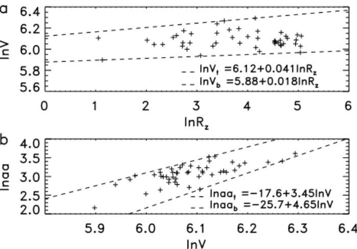
Fig. 6. (a)Scatter plot oflnV againstlnRz (pluses). The data points are all in between the two (dashed) lines oflnVt (top) and
lnVb(base).(b)Scatter plot oflnaaagainstlnV (pluses). The data
points are all in between the two (dashed) lines oflnaat(top) and
lnaab(base).
As another example, Fig. 6 shows the scatter plots of (a)lnV againstlnRzand (b)lnaaagainstlnV. One can also see that the data points in Fig. 6a are all in between the two (dashed) lines,
lnVt=6.12+0.041lnRz,
lnVb=5.88+0.018lnRz. (23)
The data points in Fig. 6b are all in between the two (dashed) lines,
lnaat = −17.6+3.45lnV ,
lnaab= −25.7+4.65lnV . (24)
Now we analyze the bivariate-fit oflnaa(solid) to bothlnRz (dashed) andlnV (dash-dotted) from 1964 to 2010, as shown in Fig. 7a. The dotted line indicates the fitted result (lnaaf), with the regression equation given by
lnaa=0.15lnRz+2.35lnV−11.79. (25) The correlation coefficient between lnaa and lnaaf (r= 0.91) is slightly higher than (r=0.89) betweenaaand the fitted result by the bivariate-fit ofaato bothRzandV.
Figure 7b shows the scatter plot of lnaa against lnaaf (pluses). It is seen that the data points are all in between two (nearly parallel) lines,
lnaat =0.17+1.01lnaaf,
lnaab=0.08+0.90lnaaf. (26)
Therefore, the solar activity (Rz) is related to the solar winds (B,V) with values being in between two certain levels, and the solar winds (B,V) are related to the geomagnetic activ-ities (aa) with values being in between another two certain levels. In turn, the solar activity (Rz) will be related to the geomagnetic activities (aa) that have a lowest and a highest
Fig. 7. (a) lnaa(solid), lnRz (dashed),lnV (dash-dotted), and the fitted resultlnaaf(dotted) by the bivariate oflnRz andlnV.
(b) Scatter plot of lnaa against lnaaf (pluses). The data points
are all in between the two (dashed) lines oflnaat(top) andlnaab
(base).
level. Two ways can also be used to decompose an index (B, V,aa) into two components according the lowest or highest level of activity, as was the case in the previous section.
The above results imply that the source activities (B,V) of aa play a role of mid-processes in the formation ofaa from solar magnetic field activity (Rz). These processes are similar to the relationship between aaandRz discussed in the previous section. The results in Figs. 5a and 6a indi-cate that the source activities (B,V) have undergone decay processes before arriving at the magnetosphere (e.g., in the solar corona). The results in Figs. 5b and 6b indicate that the interactions of these activities with the magnetosphere and ionosphere will undergo further decays when generat-ingaa. Generally speaking, the relationship betweenaaand Rz(Eq. 17) is the integrated effect of the aboveRz-B(V)-aa (andRz-CME-aa) relationships. Thus, the decay term (aad) should include the decays of solar winds (B,V), and the de-cay range (DR) may extend to the solar corona in this sense. For ease of understanding, we discussed in Sect. 4.2 the decay process mainly in the magnetosphere and ionosphere. In Sect. 4.1,Rz is assumed to be associated with a certain amount of solar energy (Et) potential of generating geomag-netic activity (aa). This statement is consistent with the sug-gestion that sunspots are related to the energy supply to the corona (de Toma et al., 2000; Temmer et al., 2003). The energy (Et) should have been related toaat(or a similar for-mula) if there were no energy loss (Ed) in the decay pro-cesses or ifEdwere all used to generateaain the same way as the transient phenomena did.
and follows the sunspot predominantly in a linear or nonlin-ear manner (aaRoraab). Another process (Et−Eb) is asso-ciated with other (recurrent) phenomena such as solar winds. The energy (Et−Eb=Eu+Ed) for the latter process has un-dergone a loss (Ed1, part ofEd) before arriving at the magne-tosphere and will undergo another loss (Ed2=Ed−Ed1) in the interactions with the magnetosphere and ionosphere. The energy loss (Ed) corresponds to the decay term (aad), which is related to solar (magnetic field) activity (Rz) because the energy (Et−Eb) is associated withRzasEbis. It is shown in Sect. 4.2 that the decayaadprecedesaa, which illustrates the fact that the generation ofaaoccurs after the decay (aad) or the energy loss (Ed). The energyEuis the remainder of Et−Eb=Eu+Ed after the (decay) lossEd. The geomag-netic activity (aau) generated byEuis almost uncorrelated withaab, which is due to the various processes in the forma-tion of bothaabandaau.
The solar energy (Et) can generate various solar activity phenomena such as solar flares, filament/prominence erup-tions, energetic protons, CMEs, and solar winds (Gosling et al., 1976; Legrand and Simon, 1989a; Feminella and Storini, 1997; Sheeley et al., 1999; Forbes et al., 2006). These ac-tivities have lost part of their energies when passing over the solar chromospheric layer and corona. It is well known that most of these activities lag behindRz from several months to a few years, which reflects the decay processes in the transmission. The energy loss (Ed1) for the decay process of one activity may generate other activities, including vari-ous electric-magnetic radiations and the variations in density and temperature of the solar chromospheric layer and corona. Therefore, most solar activities are well correlated withRz (orEt), which is the reason for the good correlation ofaad withRz. The relationships between these activities andRz are similar to that betweenaaandRzbefore arriving at the magnetosphere, as can be seen in Figs. 5a and 6a for two examples of theB-RzandV-Rzrelationships, respectively.
Similarly, the interactions of the source activities with the magnetosphere and ionosphere can also generate a series of activity phenomena such as the ring current, auroral current, and the variations in density and temperature of the Earth’s atmosphere. The energy loss (Ed2) for the decay process of one activity may generate other activities, and not all these activities are completely related toaa. The relationships be-tweenaaand these activities are similar to that betweenaa andRz, as shown in Figs. 5b and 6b for two examples of the aa-B andaa-V relationships, respectively. In summary,aa is the synthesis effect of all the above processes.
The main points of this paper may be summarized as follows:
1. The aa index is in between the two levels of aat= e2.44Rz2/7andaab=e1.36Rz2/7.
2. aa can be decomposed into two independent compo-nents: aa=aab+aau(r=0.09). aat can be divided into two independent terms:aat=aa+aad(r=0.00).
3. All theaavalues can be expressed asaa=aat−aad= e2.44±0.05−ηRz2/7±0.02 for 0≤η≤1.08, whereηrefers to the “decay index”, modulated mainly by the solar wind speed.
Acknowledgements. The authors are grateful to the anonymous ref-erees for suggestive comments, which greatly improved the present manuscript. This work is supported by the National Natural Sci-ence Foundation China through grants 10973020, 40890161, and 10921303, Chinese Academy of Sciences through grant YYYJ-1110, and National Basic Research Program of China through grant 2011CB811406.
Topical Editor R. Nakamura thanks J. Lei and another anony-mous referee for their help in evaluating this paper.
References
Bame, S. J., Asbridge, J. R., Feldman, W. C., and Gosling, J. T.: So-lar cycle evolution of high-speed soSo-lar wind streams, Astrophys. J., 207, 977–980, 1976.
Crooker, N. U., Feynman, J., and Gosling, J. T.: On the high corre-lation between long-term averages of solar wind speed and geo-magnetic activity, J. Geophys. Res., 82, 1933–1937, 1977. Demetrescu, C. and Dobrica, V.: Signature of Hale and Gleissberg
solar cycles in the geomagnetic activity, J. Geophys. Res., 113, A02103, doi:10.1029/2007JA012570, 2008.
de Toma, G., White, O. R., and Harvey, K. L.: A Picture of Solar Minimum and the Onset of Solar Cycle 23. I. Global Magnetic Field Evolution, Astrophys. J., 529, 1101–1114, 2000.
Du, Z. L.: The Relationship between Prediction Accuracy and Cor-relation Coefficient, Solar. Phys., 270, 407–416, 2011a. Du, Z. L.: The correlation between solar and geomagnetic activity
– Part 2: Long-term trends, Ann. Geophys., Ann. Geophys., 29, 1341–1348, doi:10.5194/angeo-29-1341-2011, 2011b.
Du, Z. L.: The correlation between solar and geomagnetic activity – Part 3: An integral response model, Ann. Geophys., 29, 1005– 1018, doi:10.5194/angeo-29-1005-2011, 2011c.
Du, Z. L., Li, R., and Wang, H. N.: The Predictive Power of Ohl’s Precursor Method, Astron. J., 138, 1998–2001, 2009.
Echer, E., Gonzalez, W. D., Gonzalez, A. L. C., Gonzalez, W. D., Gonzalez, A. L. C., Prestes, A., Vieira, L. E. A., Dal Lago, A., Guarnieri, F. L., and Schuch, N. J.: Long-term correlation be-tween solar and geomagnetic activity, J. Atmos. Sol. Terr. Phys., 66, 1019–1025, 2004.
Feminella, F. and Storini, M.: Large-scale dynamical phenomena during solar activity cycles, Astron. Astrophys., 322, 311–319, 1997.
Feynman, J.: Implications of solar cycles 19 and 20 geomagnetic activity for magnetospheric processes, Geophys. Res. Lett., 7, 971–973, 1980.
Feynman, J.: Geomagnetic and solar wind cycles, 1900–1975, J. Geophys. Res., 87, 6153–6162, 1982.
Feynman, J.: Reply, J. Geophys. Res., 88, 8139–8140, 1983. Feynman, J. and Crooker, N. U.: The solar wind at the turn of the
century, Nature, 275, 626–627, 1978.
Garrett, H. B., Dessler, A. J., and Hill, T. W.: Influence of solar wind variability on geomagnetic activity, J. Geophys. Res., 79, 4603–4610, 1974.
Gonzalez, W. D., Gonzalez, A. I. C., and Tsurutani, B. T.: Dual-peak solar cycle distribution of intense geomagnetic storms, Planet. Space Sci., 38, 181–187, 1990.
Gosling, J. T., Hildner, E., MacQueen, R. M., Munro, R. H., Poland, A. I., and Ross, C. L.: The speeds of coronal mass ejection events, Solar Phys., 48, 389–397, 1976.
Hathaway, D. H. and Wilson, R. M.: Geomagnetic activity indicates large amplitude for sunspot cycle 24, Geophys. Res. Lett., 33, L18101, doi:10.1029/2006GL027053, 2006.
Johnson, J. R. and Wing, S.: A solar cycle dependence of nonlinear-ity in magnetospheric activnonlinear-ity, J. Geophys. Res., 110, A04211, doi:10.1029/2004JA010638, 2005.
Leamon, R. J., Matthaeus, W. H., Smith, C. W., Zank, G. P., Mullan, D. J., and Oughton, S.: MHD-driven Kinetic Dissipation in the Solar Wind and Corona, Astrophys. J., 537, 1054–1062, 2000. Legrand, J. P. and Simon, P. A.: Ten cycles of solar and geomagnetic
activity, Solar Phys., 70, 173–195, 1981.
Legrand, J. P. and Simon, P. A.: Comment on ‘geomagnetic and solar wind cycles, 1900–1975’ by Joan Feynman, J. Geophys. Res., 88, 8137–8138, 1983.
Legrand, J. P. and Simon, P. A.: Solar cycle and geomagnetic activ-ity: A review for geophysicists. I – The contributions to geomag-netic activity of shock waves and of the solar wind, Ann. Geo-phys., 7, 565–578, 1989a.
Legrand, J. P. and Simon, P. A.: Solar cycle and geomagnetic activ-ity: A review for geophysicists. II – The solar sources of ge-omagnetic activity and their links with sunspot cycle activity, Ann. Geophys.,7, 579–593, 1989b.
Li, Y.: Predictions of the features for sunspot cycle 23, Sol. Phys., 170, 437–445, 1997.
Lukianova, R., Alekseev, G., and Mursula, K.: Effects of sta-tion relocasta-tion in the aa index, J. Geophys. Res., 114, A02105, doi:10.1029/2008JA013824, 2009.
Matthaeus, W. H., Weygand, J. M., Chuychai, P., Dasso, S., Smith, C. W., and Kivelson, M. G.: Interplanetary Magnetic Taylor Mi-croscale and Implications for Plasma Dissipation, Astrophys. J. Lett., 678, L141–L144, 2008.
Mayaud, P. N.: The aa indices: A 100-year series characterizing the magnetic activity, J. Geophys. Res., 77, 6870–6874, 1972. Nagashima, K., Fujimoto, K., and Tatsuoka, R.: Nature of
solar-cycle and heliomagnetic-polarity dependence of cosmic rays, in-ferred from their correlation with heliomagnetic spherical sur-face harmonics in the period 1976–1985, Planet. Space Sci., 39, 1617–1635, 1991.
Nevanlinna, H. and Kataja, E.: An extension of the geomagnetic ac-tivity index series aa for two solar cycles (1844–1868), Geophys. Res. Lett., 20, 2703–2706, 1993.
Papitashvili, V. O., Papitashvili, N. E., and King, J. H.: Solar cycle effects in planetary geomagnetic activity: Analysis of 36-year long OMNI dataset, Geophys. Res. Lett., 27, 2797–2800, 2000.
Richardson, I. G., Cliver, E. W., and Cane, H. V.: Sources of ge-omagnetic activity over the Solar cycle: relative importance of coronal mass ejections, high-speed streams, and slow Solar wind, J. Geophys. Res., 105, 18203–18213, 2000.
Russell, C. T. and McPherron, R. L.: Semiannual variation of geo-magnetic activity, J. Geophys. Res., 78, 92–108, 1973.
Schatten, K. H., Scherrer, P. H., Svalgaard, L., and Wilcox, J. M.: Using dynamo theory to predict the sunspot number during solar cycle 21, Geophys. Res. Lett., 5, 411–414, 1978.
Sheeley, N. R., Walters, J. H., Wang, Y.-M., and Howard, R. A.: Continuous tracking of coronal outflows: Two kinds of coronal mass ejections, J. Geophys. Res., 104, 24739–24768, 1999. Simon, P. A. and Legrand, J. P.: Solar cycle and geomagnetic
activ-ity: A review for geophysicists. II – The solar sources of ge-omagnetic activity and their links with sunspot cycle activity, Ann. Geophys.,7, 579–593, 1989.
Snyder, C. W., Neugebauer, M., and Rao, U. R.: The Solar Wind Ve-locity and Its Correlation with Cosmic-Ray Variations and with Solar and Geomagnetic Activity, J. Geophys. Res., 68, 6361– 6370, 1963.
Stamper, R., Lockwood, M., Wild, M. N., and Clark, T. D. G.: So-lar causes of the long-term increase in geomagnetic activity, J. Geophys. Res., 104, 28325–28342, 1999.
Svalgaard, L.: Geomagnetic activity: Dependence on solar wind parameters, in: Coronal Holes and High Speed Wind Streams, edited by: Zirker, J. B., Colorado Ass. U. Press, Boulder, p. 371, 1977.
Temmer, M., Veronig, A., and Hanslmeier, A.: Does solar flare activity lag behind sunspot activity? Sol. Phys., 215, 111–126, 2003.
Tsurutani, B. T., Gonzalez, W. D., Gonzalez, A. L. C., Guarnieri, F. L., Gopalswamy, N., Grande, M., Kamide, Y., Kasahara, Y., Lu, G., Mann, I., McPherron, R., Soraas, F., and Vasyli-unas, V.: Corotating solar wind streams and recurrent geo-magnetic activity: A review, J. Geophys. Res., 111, A07S01, doi:10.1029/2005JA011273, 2006.
Tu, C. Y. and Marsch, E.: MHD structures, waves and turbulence in the solar wind: observations and theories, Space Sci. Rev., 73, 1–210, 1995.
Venkatesan, D., Shulka, A. K., and Agrawal, S. P.: Cosmic ray intensity variations and two types of high speed soalr streams, Solar Phys., 81, 375–381, 1982.
Venkatesan, D., Ananth, A. G., Graumann, H., and Pillai, S.: Re-lationship between solar and geomagentic activity, J. Geophys. Res., 96, 9811–9813, 1991.