www.geosci-model-dev.net/7/2281/2014/ doi:10.5194/gmd-7-2281-2014
© Author(s) 2014. CC Attribution 3.0 License.
C-Coupler1: a Chinese community coupler for
Earth system modeling
L. Liu1, G. Yang1,2, B. Wang1,3, C. Zhang2, R. Li2, Z. Zhang2, Y. Ji2, and L. Wang4
1Ministry of Education Key Laboratory for Earth System Modeling, Center for Earth System Science (CESS),
Tsinghua University, Beijing, China
2Department of Computer Science and Technology, Tsinghua University, Beijing, China
3State Key Laboratory of Numerical Modeling for Atmospheric Sciences and Geophysical Fluid Dynamics (LASG),
Institute of Atmospheric Physics, Chinese Academy of Sciences, Beijing, China
4College of Global Change and Earth System Science, Beijing Normal University, Beijing, China Correspondence to:L. Liu ([email protected]), G. Yang ([email protected]), and B. Wang ([email protected])
Received: 9 May 2014 – Published in Geosci. Model Dev. Discuss.: 11 June 2014 Revised: 23 August 2014 – Accepted: 3 September 2014 – Published: 9 October 2014
Abstract.A coupler is a fundamental software tool for Earth system modeling. Targeting the requirements of 3-D cou-pling, high-level sharing, common model software platform and better parallel performance, we started to design and develop a community coupler (C-Coupler) from 2010 in China, and finished the first version (C-Coupler1) recently. C-Coupler1 is a parallel 3-D coupler that achieves the same (bitwise-identical) results with any number of processes. Guided by the general design of C-Coupler, C-Coupler1 en-ables various component models and various coupled mod-els to be integrated on the same common model software platform to achieve a higher-level sharing, where the compo-nent models and the coupler can keep the same code version in various model configurations for simulation. Moreover, it provides the C-Coupler platform, a uniform runtime environ-ment for operating various kinds of model simulations in the same manner. C-Coupler1 is ready for Earth system mod-eling, and it is publicly available. In China, there are more and more modeling groups using C-Coupler1 for the devel-opment and application of models.
1 Introduction
Climate system models (CSMs) and Earth system models (ESMs) are fundamental tools for the study of global cli-mate change. They play an important role in simulating and
understanding the past, present, and future climate. They are always coupled models consisting of several separate inter-operable component models to simultaneously simulate the variations of and interactions among the atmosphere, land surface, oceans, sea ice, and other components of the climate system. Following the fast development of science and tech-nology, more and more CSMs, ESMs, and related component models have appeared around the world. For example, more than 50 coupled models participated in the Coupled Model Intercomparison Project Phase 5 (CMIP5), compared to less than 30 coupled models in the previous CMIP3.
Framework (Hill et al., 2004) (ESMF), the Flexible Modeling System (FMS) coupler (Balaji et al., 2006), the CPL6 cou-pler (Craig et al., 2005) designed for the Community Climate System Model version 3 (Collins et al., 2006) (CCSM3), the CPL7 coupler (Craig et al., 2012) designed for the Com-munity Climate System Model version 4 (Gent et al., 2011) (CCSM4) and the Community Earth System Model (Hurrell et al., 2013) (CESM), and the Bespoke Framework Genera-tor (Ford et al., 2006; Armstrong et al., 2009) (BFG). Most of these couplers provide typical coupling functions (Valcke et al., 2012a), such as transferring coupling fields between com-ponent models, interpolating coupling fields between differ-ent grids of compondiffer-ent models, and coordinating the execu-tion of component models in a coupled model.
Regarding the future development of CSMs and ESMs, we would like to highlight the following ongoing requirements for coupler development:
1. 3-D coupling. Generally, coupling occurs on the com-mon boundaries or domains between component mod-els. In CSMs, most common interfaces between any two component models are on 2-D horizontal surfaces. For example, the common surface between an atmosphere model and an ocean model is on the skin of the ocean, which is also the bottom of the atmosphere. A CSM also needs 3-D coupling – for example, between physics and dynamics in an atmosphere model. In ESMs, compo-nent models can share the same 3-D domain. For ex-ample, both atmospheric chemistry models and atmo-sphere models simulate in the 3-D atmoatmo-sphere space. When coupling them together, especially when their 3-D grids are different, 3-3-D coupling, including transfer-ring and interpolating 3-D coupling fields, needs to be achieved. Some existing couplers, such as the OASIS coupler, MCT, the CPL6 coupler, the CPL7 coupler and ESMF, already provide 3-D coupling functions. 2. High-level sharing. A component model can be shared
by different coupled model configurations for various scientific research purposes. In different coupled model configurations, the same component model may have different coupling fields and different common inter-faces with other component models. For example, given an atmosphere model, when it is used as a stand-alone component model, there are no coupling fields. When it is used as a component of a CSM, it will provide/obtain 2-D coupling fields for/from other component mod-els. When it is coupled with an atmospheric chemistry model, some 3-D variables with vertical levels become coupling fields. In each coupled model configuration, the atmosphere model can have a branch code version with a specific procedure for providing/obtaining the corresponding coupling fields. When more and more coupled model configurations share the atmosphere model, there will be an increasing number of branch code versions, which will introduce more complexity
into the code version control. To facilitate the code ver-sion control for sharing a component model, the coupler should enable multiple configurations of coupled mod-els without requiring source code changes to the indi-vidual component models and the coupler itself. 3. To develop a model or to achieve a scientific research
target, scientists always need to run various kinds of models. For example, to develop an atmosphere model, scientists may want to use various combinations of a single-column model of physical processes, a stand-alone atmosphere model, an air–sea coupled model, a nested model, a CSM, or an ESM. Moreover, scien-tists may want to cooperatively use the models from dif-ferent groups or institutions for a scientific purpose. If the software platforms for these models are not identi-cal, scientists have to invest a lot of effort into learn-ing how to handle model simulations on each platform. To facilitate model development and scientific research, a coupler should be able to integrate various compo-nent models and various coupled models on a common model software platform which handles various kinds of model simulations in the same manner, i.e., the same way for creating, configuring, compiling, and running model simulations.
4. Better parallel performance. In the future, the coupler’s functions will become more computationally expensive for Earth system modeling in several aspects. First, the coupler will be required to manage the coupling be-tween more and more component models in a coupled model configuration. Second, 3-D coupling will intro-duce much higher communication and calculation over-head than 2-D coupling. Third, the resolution of compo-nent models coupled together will continually increase. Therefore, it will be increasingly important to improve the parallel performance of a coupler.
different coupling architectures, and made these model con-figurations share the same code of the component models and C-Coupler1, as well as the same C-Coupler platform for sim-ulation.
In this paper, we will introduce the general design of C-Coupler and show details of C-C-Coupler1. The remainder of this paper is organized as follows: Sect. 2 briefly introduces existing couplers, Sect. 3 presents the general design of C-Coupler, Sect. 4 presents C-Coupler1 in detail, Sect. 5 empir-ically evaluates C-Coupler1, and Sect. 6 discusses the future works for the development of C-Coupler. We conclude this paper in Sect. 7.
2 Brief introduction to existing couplers
In this section, we will briefly introduce the OASIS coupler; MCT; ESMF; the FMS, CPL6, and CPL7 couplers; and BFG. More details of these couplers can be found in Valcke et al. (2012a), Redler et al. (2010), Valcke (2013a), Larson et al. (2005), Jacob et al. (2005), Hill et al. (2004), Balaji et al. (2006), Craig et al. (2005, 2012), Ford et al. (2006), and Armstrong et al. (2009).
2.1 The OASIS coupler
The European Centre for Research and Advanced Train-ing in Scientific ComputTrain-ing (CERFACS, Toulouse, France) started to develop the OASIS coupler in 1991. OASIS3 (Val-cke, 2013a) is a 2-D version of the OASIS coupler. It has been widely used for developing the European CSMs and ESMs. For example, it has been used in different versions of five European CSMs and ESMs that have participated in CMIP5, e.g., CNRM-CM5 (Voldoire et al., 2011), IPSL-CM5 (Dufresne et al., 2013), CMCC-ESM (Vichi et al., 2011), EC-Earth V2.3 (Hazelger et al., 2011), and MPI-ESM (Giorgetta et al., 2013; Jungclaus et al., 2013). OA-SIS3 uses multiple executables for a coupled model, where OASIS3 itself forms a separate executable for data interpola-tion tasks and each component model remains a separate ex-ecutable. It provides an ASCII-formatted “namcouple” con-figuration file, which is an external concon-figuration file written by users, to specify some characteristics of each coupling ex-change, e.g. source component, target component, coupling frequency, and data-remapping algorithm. For data interpo-lation, OASIS3 can use the remapping weights generated by the 2-D remapping algorithms in the Spherical Coordi-nate Remapping and Interpolation Package (SCRIP) library (Jones, 1999). The degree of parallelism of OASIS3 is lim-ited to the number of coupling fields, because each process for OASIS3 is responsible for a subset of the coupling fields. OASIS4 is a 3-D version of the OASIS coupler, which supports both 2-D and 3-D coupling. Similar to OASIS3, OASIS4 also uses multiple executables for a coupled model and can use SCRIP for 2-D interpolation. It also provides a
“namcouple” configuration file, and the configuration is de-scribed in an XML format. As a 3-D coupler, OASIS4 sup-ports transfer and interpolation for 3-D fields. For 3-D inter-polation, OASIS4 itself provides pure 3-D remapping algo-rithms, e.g., 3-Dnneighbor distance-weighted average and trilinear remapping algorithms, and supports 2-D interpola-tion in the horizontal direcinterpola-tion followed by a linear inter-polation in the vertical direction. In July 2011, CERFACS stopped the development of OASIS4 and started to develop a new coupler version, OASIS3-MCT (Valcke et al., 2012b; Valcke, 2013b), which further improves the parallelism of OASIS3.
In the following context, we use “namcouple” and “code-couple” to respectively denote the way of specifying charac-teristics of coupling in configuration files and in source code.
2.2 The Model Coupling Toolkit
The Model Coupling Toolkit (MCT) provides the fundamen-tal coupling functions: data transfer and data interpolation, in parallel. MCT represents a coupling field into a 1-D ar-ray and uses sparse matrix multiplication to achieve data in-terpolation. Therefore, it can be used for both 2-D and 3-D coupling. For 2-3-D interpolation, MCT can use remapping weights generated by SCRIP. However, it rarely achieves 3-D interpolation due to the lack of 3-D remapping weights gen-erated by existing remapping software. As a result, MCT is not user-friendly enough in 3-D coupling and users always have to implement 3-D interpolation in the code of compo-nent models.
MCT can be viewed as a library for model coupling. It can be directly used to couple fields between two component models where no separate executable is generated for cou-pling tasks, and can also be used to develop other couplers, e.g., OASIS3-MCT, the CPL6 coupler and the CPL7 coupler. 2.3 The Earth System Modeling Framework
average, and 3-D first-order conservative. For parallelism, the ESMF can remap data fields in parallel and keep bitwise-identical results when changing the number of processes for interpolation.
In CMIP5, the coupled model NASA GEOS-5 uses ESMF throughout, and the coupled models CCSM4 and CESM1 use the higher-order patch recovery remapping algorithm pro-vided by the ESMF.
2.4 The FMS coupler
The Flexible Modeling System (FMS) is a software frame-work that is mainly developed by and used in the Geophysi-cal Fluid Dynamics Laboratory (GFDL) for the development, simulation and scientific interpretation of atmosphere mod-els, ocean modmod-els, CSMs, and ESMs. The coupling between component models in the FMS is achieved by the FMS pler in parallel. Similar to MCT and ESMF, the FMS cou-pler uses “codecouple” configuration for model coupling, and can keep bitwise-identical result across different paral-lel decompositions. One key feature of the FMS coupler is the “exchange grid” (Balaji et al., 2006). Given two compo-nent models, the corresponding exchange grid is determined by all vertices in the two grids of these two component mod-els, and the coupling between these two component models is processed on the exchange grid. For example, the coupling fields from the source component model are first interpolated onto the exchange grid and then averaged onto the grid of the target component model. In CMIP5, the CSMs and ESMs (Donner et al., 2011; Dunne et al., 2012) from the GFDL use the FMS as well as its coupler.
2.5 The CPL6 coupler
The CPL6 coupler is the sixth version in the coupler family developed at the National Center for Atmospheric Research (NCAR). It is a centralized coupler designed for CCSM3, where the atmosphere model, land surface model, ocean model, and sea ice model are connected to the unique coupler component and the coupling between any two component models is performed by the coupler component. Through in-tegrating MCT, the CPL6 coupler achieves the data trans-fer and data interpolation in parallel. Moreover, it provides a number of numerical algorithms for calculating and merg-ing some fluxes and state variables for component models. It uses multiple executables for a coupled model, where the coupler component forms a separate executable. Similar to MCT, the CPL6 coupler uses “codecouple” configuration for model coupling. For data interpolation, it always uses the remapping weights generated by SCRIP.
In CMIP5, the CPL6 coupler, as well as the model plat-form of CCSM3, has been widely used in Chinese cou-pled model versions, e.g., FGOALS-g2 (Li et al., 2013a), FGOALS-s2 (Bao et al., 2013), BNU-ESM (Ji et al., 2014), BCC-CSM, and FIO-ESM.
2.6 The CPL7 coupler
The CPL7 coupler is the latest coupler version from NCAR. It has been used for the CMIP5 models CCSM4 and CESM1. It keeps most of the characteristics from the CPL6 cou-pler, such as a centralized coupler component, integration of MCT, and flux computation. The most notable advance-ments from the CPL6 coupler to the CPL7 coupler include the following: (1) the CPL7 coupler does not use multiple executables but single executable for a coupled model and provides a top-level driver to achieve various processor lay-out and time sequencing of the components in order to im-prove the overall parallel performance of the coupled model, and (2) a parallel input/output (I/O) library is implemented in the CPL7 coupler to improve the I/O performance.
2.7 The Bespoke Framework Generator
The Bespoke Framework Generator (BFG) aims to make the coupling framework more flexible in model composi-tion and deployment. BFG2 is the latest version of BFG. It provides a metadata-driven code generation system where a set of XML-formatted metadata is designed for gener-ating the wrapper code of a coupled model configuration. BFG metadata are classified into three phases: model defi-nition, composition, and deployment. The model definition metadata describe the implementation rules of each com-ponent model, including <name>,<type>, <language>, <timestep>, and<entryPoints>. The<entryPoints> con-sist of a set of entry points each of which corresponds to a user-specified subprogram unit that can be called by the main program in a coupled model. An entry point can con-tain a number of <data> elements, each of which corre-sponds to an argument of the entry point. When a<data> el-ement represents an array, the number of dimensions and the bounds for each dimension need to be specified. The com-position metadata specify how component models are cou-pled together with a number of<set>elements. Each<set> element identifies references to a coupling field, where the references are arguments of the corresponding entry points. The deployment metadata specify how the coupled model is mapped onto the available hardware and software resources. BFG2 designs a “namcouple” approach to separate the code of models from the coupling infrastructure. Although it does not provide coupling functions such as data inter-polation, it enables users to choose the underlying coupling functions from other couplers, such as the OASIS coupler. As models are not main programs in a coupled model with BFG2, a single executable or multiple executables can be se-lected for deploying a coupled model.
2.8 Summary
couplers. However, these 3-D coupling functions should be further improved. The 3-Dnneighbor distance-weighted av-erage, trilinear, and linear remapping algorithms used in the OASIS coupler and ESMF can result in low accuracy in the interpolation on the vertical direction. MCT, the CPL6 cou-pler, and the CPL7 coupler generally cannot interpolate in 3-D due to a lack of remapping weights. Moreover, most exist-ing couplers use sparse matrix multiplication to achieve data interpolation. Limited by this implementation, some higher-order remapping algorithms for the 1-D vertical direction, such as spline, cannot be used in 3-D interpolation, because these algorithms cannot be achieved purely by sparse matrix multiplication.
Existing couplers that use “codecouple” configuration, e.g., MCT, ESMF, and the FMS, CPL6, and CPL7 couplers, are not convenient for sharing the same code version of cou-pler and component models among various coupled model configurations. For example, when increasing coupling fields or component models based on a coupled model configu-ration, the code of coupler or component models has to be modified. Although some model code could have compiler directives (such as “#ifdef”) for different coupled model con-figurations, heavy use of compiler directives will make the model code hard to be read and maintain for further devel-opment, and the change in coupled model configuration re-quires a recompiling of model code. Regarding the OASIS coupler, its “namcouple” configuration, which specifies how to transfer and interpolate each coupling field, can decrease code modification requirements when changing the corres-ponding characteristics of coupling. However, the configura-tion files in the OASIS coupler do not specify external al-gorithms for calculating coupling fields, such as flux lation algorithms. When changing the procedures for calcu-lating coupling fields, the code of component models always has to be modified. Regarding BFG, its metadata can further describe and manage user-specified subprogram units. How-ever, the wrapper code needs to be regenerated and recom-piled whenever the metadata changes. Moreover, the descrip-tion of an array, which specifies the number of dimensions and the bounds for each dimension, is not flexible enough for changing parallel decompositions of models.
There are several model software platforms correspond-ing to existcorrespond-ing couplers which have been successfully used for model development, such as the CCSM3 platform cor-responding to the CPL6 coupler, the CCSM4/CESM plat-form corresponding to the CPL7 coupler, and the FMS. These platforms can configure, compile, and run differ-ent kinds of model configurations for simulation. The CCSM4/CESM platform can run stand-alone component models, CSMs, ESMs, etc. However, to make a new stand-alone component model run on the CCSM4/CESM plat-form, users have to dramatically modify the code of the component model. For example, when integrating an ocean model version, i.e., MOM4p1 (Griffies et al., 2010), onto the CCSM4/CESM platform for a stand-alone ocean model
configuration without coupling with other component mod-els, the code of MOM4p1 needs to be dramatically modified to use the CPL7 coupler as the driver.
Improving parallel performance is always a focus in cou-pler development. It concerns the parallel performance of both the coupler and the whole coupled model. Similarly, we are concerned with the parallel performance of both the coupler and coupled models in the long-term development of C-Coupler.
3 General design of C-Coupler
In this section, we will briefly introduce the general design of C-Coupler. C-Coupler can be viewed as a family of the community coupler developed in China, and C-Coupler1 is the first version following the general design. The future ver-sions of C-Coupler will also follow the general design. In the following context, we first define a general term,experiment model, and then introduce the architecture of the experiment models with C-Coupler and the general software architecture of C-Coupler.
3.1 A general term for C-Coupler: experiment model
An experiment model is a model configuration which can run on the C-Coupler platform for simulations. It consists of a certain set of configuration files and a certain set of model code, with a certain set of rules for precompiling. Generally, an experiment model can be any kind of model configur-ation, such as a single-column model, a stand-alone compo-nent model, a regional coupled model, an air–sea coupled model, a nested model, a CSM, an ESM, etc.
3.2 Architecture of the experiment models with C-Coupler
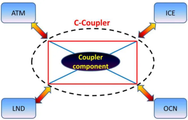
To achieve the target of integrating various models on the same common model software platform for a high-level shar-ing of the component models and for facilitatshar-ing the con-struction of a new experiment model, we have designed an architecture for the experiment models with C-Coupler. Fig-ure 1 shows an example of this architectFig-ure with a typical CSM, where “ATM”, “ICE”, “LND”, and “OCN” stand for the component models. The key ideas of this design include the following:
Figure 1.The architecture of the models with C-Coupler.
transfer, data interpolation, and flux computation, are performed through the uniform C-Coupler application programming interfaces (APIs) called by the component models. Compared to the approach with a separate cou-pler component, direct coupling can reduce the number of data transfers for better parallel performance, but it can lower code modularity. Users can select a separate coupler component, direct coupling, or hybrid for con-structing a coupled model configuration. For example, users can use a separate coupler component for a CSM or ESM for better code modularity and use direct cou-pling for an air–sea coupled model for better parallel performance.
2. When a component model is shared by multiple experi-ment models, it keeps the same code version in all these experiment models. The code of coupling interfaces in the component model only specifies the input fields that the component model wants and the output fields that the component model can provide, but does not specify how to get the input fields and how to provide the out-put fields. For example, the source component models, the target component models, and the flux calculation of the coupling fields are not specified in the code of the coupling interfaces.
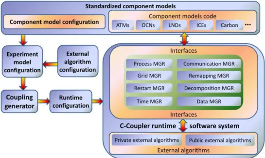
3.3 General software architecture of C-Coupler Under the guidance of the key ideas, we designed the gen-eral software architecture of C-Coupler, which consists of a configuration system, a runtime software system, and a cou-pling generator, as shown in Fig. 2. In the following context of this subsection, we will further introduce the configuration system and runtime software system. The coupling generator that has not been developed in C-Coupler1 will be further discussed in Sect. 6.
3.3.1 Configuration system
In different experiment models, a component model always has different procedures for the input and output fields. For example, given an atmosphere model, in its stand-alone com-ponent model configuration, the ocean surface state fields (such as sea surface temperature) are obtained from the I/O data files, while in an air–sea coupled model config-uration, the ocean surface state fields are obtained from the ocean model through coupling. Moreover, in these two model configurations, the algorithms for computing the air– sea flux (such as evaporation, heat flux, and wind stress) can be different. To make the same code version of a compo-nent model shared by various experiment models, C-Coupler should make a procedure adaptively achieve different func-tions for different model configurafunc-tions without code mod-ification. We therefore designed a configuration system in C-Coupler. Besides the functionality achieved by the “nam-couple” configuration file in the OASIS coupler and BFG, the configuration system of C-Coupler can further specify procedures for coupling. In the following context of this pa-per, we call such proceduresruntime procedures. A runtime procedure consists of a list of algorithms calledruntime al-gorithms. The runtime algorithms can be classified into two categories: internal algorithms and external algorithms. The internal algorithms are implemented within C-Coupler, in-cluding the data transfer algorithms, data-remapping algo-rithms, data I/O algoalgo-rithms, etc. The external algorithms are always provided by the component models, coupled models, and users. They could be the private algorithms of a compo-nent model or common algorithms such as flux calculation algorithms which can be shared by various experiment mod-els.
The configuration system manages the configuration files of software modules and the runtime configuration files of model simulations. The software modules include compo-nent models, experiment models, and external algorithms. In detail, the configuration files of a component model specify some characteristics of the component model, e.g., the input and output fields, how to generate the input namelists, and how to compile the code of the model. The configuration files of an experiment model specify how to organize the compo-nents, e.g., the components in the experiment model and how each component gets the input fields and provides the output fields. The configuration files of an external algorithm spec-ify the input and output fields of the algorithm. The runtime configuration files specify how to run an experiment model for a simulation, e.g., how to organize the internal algorithms and external algorithms into the runtime procedures for the input and output fields of the components, the coupling fre-quencies, and the start time and stop time of the simulation.
Figure 2.The general software architecture of C-Coupler.
more easily understood. When a runtime procedure is called by model code, the function pointer (some programming lan-guages such as C++ support function pointers) corresponding to each runtime algorithm will be found according to the key-word and then the runtime algorithms can be executed one by one. As the function pointer of a runtime algorithm needs to be searched only one time during the whole simulation, the extra overhead introduced by the approach of the runtime procedure is trivial. The same runtime procedure can achieve different functions in different model configurations through modifying the list of runtime algorithms that is recorded in a configuration file, without modification of model code.
3.3.2 Runtime software system
The runtime software system can be viewed as a common, flexible, and extendible library for constructing experiment models and for running model simulations. It enables various kinds of experiment models to share the same code of C-Coupler.
First, it provides a set of uniform APIs for integrating component models. With these APIs, a component model can register the model grids, parallel decompositions and I/O fields, and get/put the I/O fields from/into I/O data files or other components, etc.
Second, similar to the ESMF, the runtime software sys-tem supports the registry of functions in a coupled syssys-tem. It provides uniform APIs for integrating external algorithms. A component model can register its private subroutines as external algorithms of C-Coupler. Common algorithms like flux calculation algorithms can also be registered as external algorithms. Therefore, the runtime software system is an ex-tendible library which can integrate more and more common
external algorithms, and thus users can have more choices for model simulations. For example, given an air–sea coupled model, if there are several different algorithms for calculat-ing air–sea flux, users can select one of them in a simulation, or two or more of them for sensitivity experiments.
into the restart I/O data files when the timer for the restart writing is on. The runtime process manager manages the in-ternal algorithms and the registered exin-ternal algorithms, or-ganizes these runtime algorithms into a number of runtime procedures, and executes the runtime procedures in a model simulation.
Modularity is an important characteristic of software qual-ity. A coupler is a software tool for improving modularity of coupled models. The software architecture with a set of managers targets better modularity of the runtime software system. It can enhance the independence of each manager, so as to facilitate the advancement of C-Coupler. For exam-ple, when one manager is upgraded, the whole C-Coupler is upgraded. Moreover, it can enhance the testing and reliabil-ity for each manager. For example, diagnoses can be inserted into the source code of C-Coupler for detecting potential er-rors in the input and output of a manager.
4 C-Coupler1: first released version of C-Coupler C-Coupler1 is the first version of C-Coupler for public use. Many ideas and concepts from existing couplers have been considered for its design and implementation. As the ini-tial version of C-Coupler, it does not include the coupling generator. However, we carefully developed the configura-tion system and the runtime software system, which makes C-Coupler1 achieve most of the characteristics in the general design of C-Coupler and reach the target of sharing the same code version of C-Coupler and component models among different experiment models. Moreover, we designed and de-veloped the C-Coupler platform, which enables users to op-erate various model simulations in the same manner.
C-Coupler1 is a 3-D coupler, where the coupling fields can be 0-D, 1-D, 2-D, or 3-D. It uses multiple executables for the coupled models, each component of which has a sepa-rate executable. It can be used to construct a simple coupler component with a few lines of code, and can also be used for direct coupling between component models without separate executables specifically for the coupling tasks. It does not use the “codecouple” configuration but develops a powerful configuration system. As it is a 3-D coupler, it can interpo-late both 2-D and 3-D fields. The runtime software system of C-Coupler1 has been parallelized using the Message Passing Interfaces (MPI) library, while the bitwise-identical result is kept when changing the number of processes for C-Coupler1. In the following context of this section, we will present the runtime software system, configuration system, and C-Coupler platform in C-C-Coupler1, and then introduce how to couple a component model and the enhancement for reliabil-ity of software.
4.1 The runtime software system
The runtime software system is a parallel software library programmed mainly in C++ for better code modularity. It provides APIs mainly in Fortran, because most component models for Earth system modeling are programmed in For-tran. In the following context, we will introduce the technical features of the runtime software system, including the APIs, each manager, and parallelization.
4.1.1 The APIs
Table 1 lists out the APIs provided by C-Coupler1, which can be classified into four categories: the main driver, reg-istration, restart function, and time information. Besides the brief description of each API in Table 1, we would like to fur-ther introduce two APIs:c_coupler_execute_procedure and c_coupler_register_model_algorithm.
The APIc_coupler_execute_proceduretakes the name of a runtime procedure as an input parameter, while the algo-rithm list for the runtime procedure is specified in the cor-responding runtime configuration files. Thus, a runtime pro-cedure can keep the same name in various experiment mod-els, and users can make the same runtime procedure perform different tasks through modifying the runtime configuration files that can be viewed as a part of input of a model simula-tion. As a result, a component model can keep the same code version in various experiment models sharing it.
Almost all APIs are in Fortran except
the c_coupler_register_model_algorithm. The
c_coupler_register_model_algorithm is in C++
be-cause most Fortran versions do not support function pointer. A private external algorithm (or subroutine) registered by a component model through this API does not have explicit input and output fields. The input and output of such a algorithm are specified implicitly in the code (always Fortran code) through use of public variables of component models. In the future version of C-Coupler, we may enable the private external algorithms to have explicit input and output fields.
4.1.2 The implementation of managers The communication manager
The communication manager adaptively allocates and man-ages the MPI communicators for the MPI communications within and between the components of an experiment model. It also provides some utilities for other managers, such as getting the ID of a process in the communicator of a compo-nent or in the global communicator.
The grid manager
Table 1.The APIs provided by C-Coupler1.
Classification API Brief description
Main driver c_coupler_initialize This API initializes the runtime software system. A component model can obtain its MPI communicator with this interface.
c_coupler_finalize This API finalizes the runtime software system.
c_coupler_execute_procedure This API invokes the runtime software system to run the correspond-ing runtime procedure which consists of a list of runtime algorithms specified by the corresponding runtime configuration files. The cor-responding runtime procedure could be empty without any runtime algorithms. A component model can have multiple different runtime procedures.
Registration c_coupler_register_model_data This API registers a field of component model to enable the runtime software system to access the memory space of this field.
c_coupler_withdraw_model_data This API withdraws a field of component model from the runtime software system which has been registered before.
c_coupler_register_decomposition This API registers a parallel decomposition to the runtime software system. A component model can register multiple different parallel decompositions, even on the same horizontal grid.
c_coupler_register_model_algorithm This API registers an algorithm (also known as a subroutine) of a com-ponent model as an external algorithm of the runtime software system. Restart function c_coupler_do_restart_read This API reads in the data value of fields in a restart run of a model
simulation.
c_coupler_do_restart_write This API writes out the data value of fields for restart run. Time information c_coupler_get_current_calendar_time This API gets the calendar time of the current step.
c_coupler_get_nstep This API gets the number of the current step from the start of the model simulation.
c_coupler_get_num_total_step This API gets the number of total steps of the model simulation. c_coupler_get_step_size This API gets the number of seconds of the time step.
c_coupler_is_first_restart_step This API checks whether the current step is the first step of a restart run.
c_coupler_is_first_step This API checks whether the current step is the first step of an initial run, which also means whether the number of the current step is 0. c_coupler_advance_timer This API advances the time of simulation.
c_coupler_check_coupled_run_finished This API checks whether the model simulation ends.
c_coupler_check_coupled_run_restart_time This API checks whether the current step is time for writing fields into I/O data files for restart run.
c_coupler_get_current_num_days_in_year This API gets the number of days elapsed since the first day of the current year.
c_coupler_get_current_year This API gets the year of the current step. c_coupler_get_current_date This API gets the date of the current step. c_coupler_get_current_second This API gets the second of the current step. c_coupler_get_start_time This API gets the start time of the model simulation c_coupler_get_stop_time This API gets the end time of the model simulation. c_coupler_get_previous_time This API gets the time of the previous step. c_coupler_get_current_time This API gets the time of the current step.
c_coupler_get_num_elapsed_days_from_start This API gets the number of days elapsed since the start time of the model simulation.
c_coupler_is_end_current_day This API checks whether the current step is the last step of the current day.
b; it can be downloaded through “svn–username=guest– password=guest co http://thucpl1.3322.org/svn/coupler/ CoR1.0”) to manage the grids with dimensions from 1-D to 4-D. In a model simulation, the grids of component models are registered to the grid manager with a script of CoR, where the grid data (such the latitude, longitude and mask corresponding to each grid cell) are always read from I/O data files. Besides the support of multiple dimensions of grids, another advantage of using CoR for grid management is that it can detect the relationship between to two grids; for example, a 2-D grid is the horizontal grid of a 3-D grid with vertical levels. Moreover, for horizontal 2-D grid, CoR can support logically rectangular and unstructured grids, such as a cubic spherical grid.
The parallel decomposition manager
Most of component models for Earth system modeling have been parallelized using the MPI library, where the whole do-main of each component model, which always is a 3-D grid with vertical levels, is decomposed into a number of subdo-mains for parallelization and each process of the component model is responsible for a subdomain. We refer to the decom-position from the whole domain into subdomains as parallel decomposition. In C-Coupler1, each parallel decomposition managed by the parallel decomposition manager is based on a 2-D horizontal grid that has been registered to the grid man-ager; the parallel decomposition on the vertical subgrid of the 3-D grid is not yet supported. To register a parallel decom-position, C-Coupler1 uses an implementation derived from MCT: each process of a component model enumerates the global index (the unique index in the whole domain) of each local cell (each cell in the subdomain of this process) in the corresponding horizontal grid. A component model can reg-ister multiple parallel decompositions on the same horizontal grid, while each parallel decomposition has a unique name which is treated as the keyword of it.
The remapping manager
The remapping manager utilizes CoR to achieve the data interpolation function. There are several remarkable advan-tages of using CoR for interpolation. First, it can help the Coupler1 to remap the field data on 1-D, 2-D, and 3-D grids. Second, it can generate remapping weights using its inter-nal remapping algorithms and can also use the remapping weights generated by other software, such as SCRIP. Third, it is designed to be able to interpolate field data between two grids with any structures, which makes C-Coupler1 able to be used more extensively. Similar to other couplers such as the OASIS coupler, MCT, ESMF, and the CPL6/CPL7 coupler, C-Coupler1 can utilize the remapping weights generated of-fline by remapping software such as CoR and SCRIP. The I/O data files for the offline remapping weights are specified in a script of CoR, the same script for registering the grids.
In different simulations of the same experiment model, users can select different remapping algorithms through modifying the script.
Considering that the vertical grids (such as a sigma-p grid) of component models may be changed during the model ex-ecution, the 1-D remapping weights for the “2-D+1-D” in-terpolation can be generated online in parallel by C-Coupler1 in the execution of a model simulation. This online weight generation can scale well because the vertical grid is not de-composed for parallelization and each process can generate the 1-D remapping weights independently.
CoR makes C-Coupler1 more flexible in 3-D interpolation when compared with existing couplers. First, CoR supports the “2-D+1-D” approach to interpolate data between two
3-D grids, where a 2-D remapping algorithm is used for the interpolation between the 2-D horizontal subgrids and a 1-D remapping algorithm is used for the interpolation between the 1-D vertical subgrids. Given that there areM2-D remap-ping algorithms andN 1-D remapping algorithms, there are M×N selections for 3-D interpolation. Second, CoR sup-ports both sparse matrix multiplication and equation group solving for interpolation calculation. Thus, it can provide some higher-order remapping algorithms, such as spline, that require a tri-diagonal equation group to be solved. Moreover, it makes C-Coupler1 able to handle some unstructured grids. For example, when the source grid is a cubic spherical grid, the bilinear remapping algorithm in SCRIP cannot be used, while CoR can handle this case.
The timer manager
The timer manager coordinates the component models in a coupled model to advance the simulation time in an orderly. In the runtime software system, each coupling field can have a set of timers for periodically triggering the operations on it. For example, a coupling field always has a timer for data transfer and a timer for data interpolation. Moreover, each external algorithm has a timer to periodically trigger its ex-ecution. There are three elements in a timer: the unit of fre-quency, the count of frefre-quency, and the count of delay. The unit and the count of frequency specify the period of the timer. The count of delay specifies a lag of the time during which the corresponding operation or algorithm will not be executed. The unit of frequency can be “years”, “months”, “days”, “seconds”, and “steps”, where “steps” means the time step of calling the API c_coupler_advance_timer. For example, the timer <10, steps, 15>means that the corre-sponding operation or algorithm will be executed at the steps with number 10×N+15, whereNis a nonnegative integer. Sequential and concurrent runs between component models can be achieved through cooperatively setting the delay of the timers.
Besides managing all the timers, the timer manager pro-vides interfaces for getting the information of model time (e.g., calendars) during a simulation.
The data manager
The fields managed by the data manager include the external fields which are registered by the components with APIs and the internal fields which are automatically allocated by the data manager. A coupling field, such as sea surface temper-ature (SST), can have different instances in a coupled model configuration due to different parallel decompositions and different grids. There is a keyword for each field instance, which consists of the name of the field, the name of the cor-responding component model, the name of the ing parallel decomposition, and the name of the correspond-ing grid. To define a field instance, the correspondcorrespond-ing four names must have been defined or registered to the runtime software system. For an external field instance, these four names are specified when a component model registers this field instance through calling the corresponding API, while for an internal field instance, these four names are specified in configuration files. For the scalar field which is not on a grid, the corresponding parallel decomposition and grid are marked as “NULL”.
All instances of a coupling field share the same field name. The field values in one instance can be transformed into an-other instance through data transferring between two com-ponent models and data interpolation within a comcom-ponent model. All component models in a coupled model share the names of the coupling fields. All legal field names are listed in the configuration files, with other attributes such as the
long name (also known as the description of the field) and the unit.
The data manager achieves several advantages beyond ex-isting solutions. First, a 2-D field and a 3-D field can share the same 2-D parallel decomposition, while their correspond-ing grids are different, where the 2-D grid correspondcorrespond-ing to the 2-D field is a subgrid of the 3-D grid corresponding to the 3-D field. Second, the data manager unifies the manage-ment of different kinds of field instances, such as with dif-ferent grids, difdif-ferent parallel decompositions, and difdif-ferent data types (i.e., integer and floating point). As a result, the data transfer algorithm can transfer different kinds of field instances at the same time for better communication perfor-mance. Third, the data manager helps improve the reliability for model coupling. For example, the remapping manager can examine whether the grids of source fields and target fields match the grids of the remapping weights.
The restart manager
For reading/writing fields from/into the restart I/O data files, the restart manager iterates on each field managed by the data manager. For the internal fields, the restart manager can auto-matically detect the fields which are necessary for restarting the model simulation. For an external field, the correspond-ing component can specify whether this field is necessary for restarting when registering it with the C-Coupler API. As a result, a component model has more selections for achiev-ing the restart function. It can still use its own restart system or register all fields for restart as external fields to the data manager.
The runtime process manager
The runtime process manager is responsible for running the list of runtime algorithms in each runtime procedure during a model simulation. Besides the external algorithms, including the private algorithms registered by the component models and the common flux calculation algorithms, there are several algorithms internally implemented in the runtime software system, e.g., the data transfer algorithm, data-remapping al-gorithm, and data I/O algorithm. The data transfer algorithm is responsible for transferring a number of fields from one component to another. The fields transferred by the same data transfer algorithm can have different number of dimensions, different data types, different parallel decompositions, differ-ent grids, differdiffer-ent frequency of transfer, etc. The data trans-fer algorithm packs all fields that are to be transtrans-ferred at the current time step into one package to improve the communi-cation performance.
timer, while the data types (i.e., single-precision and double-precision floating point) can be different.
The data I/O algorithm currently utilizes the serial I/O to read/write multiple fields which are managed by the data manager from/into the data I/O files. The multiple fields in a data I/O algorithm share the same timer, but they can have different parallel decompositions, different grids, and differ-ent data types. The fields of a data I/O algorithm are speci-fied in the corresponding runtime configuration file. For the future version of C-Coupler, we will further improve the I/O performance with parallel I/O for higher-resolution models. 4.1.3 Parallelization
As previously mentioned, the runtime software system has been parallelized using the MPI library and achieves bitwise-identical results when changing the number of processes. Here we would like to further introduce some details, includ-ing the parallelization of the data transfer algorithm, the par-allelization of the data-remapping algorithm, and the default parallel decomposition.
Parallelization of the data transfer algorithm
This parallelization is derived from existing couplers such as MCT. For a coupling field instance transferred by the data transfer algorithm, it has a parallel decomposition in the source component and another parallel decomposition in the target component, and these two parallel decompositions share the same horizontal grid. A process in the source com-ponent will transfer the data of this field to a process in the target component only when the corresponding subdomains on these two processes have common cells. As this imple-mentation does not involve collective communications and there are always multiple processes to execute the source component and the target component, the data transfer al-gorithm can transfer the coupling fields in parallel.
Parallelization of the data-remapping algorithm
The data-remapping algorithm interpolates a number of fields from the source grid to the target grid. To cause the fields to be interpolated in parallel, C-Coupler1 uses an ap-proach from MCT, which generates an internal parallel de-composition for rearranging coupling fields before interpo-lating. The internal parallel decomposition is on the source grid and determined by the remapping weights and the par-allel decomposition corresponding to the target grid. For ex-ample, given that global cellyof the target grid is assigned to processp, and given a remapping weight< x, y, w >, where x specifies a global cell in the source grid andwis a weight value, the internal parallel decomposition for processpwill include the global cellx of the source grid. After rearrang-ing the fields accordrearrang-ing to the internal parallel decomposition using the data transfer algorithm, process pcan interpolate the fields locally. This implementation avoids the reduction
for sum between multiple processes of a component model so as to make the data-remapping algorithm achieve bitwise-identical results when using different numbers of processes. Although it can increase the overhead when rearranging cou-pling fields, the collective communication for the reduction for sum between multiple processes can be avoided. Default parallel decomposition
In an experiment model, not all parallel decompositions are specified by the component models through registration. For example, the parallel decompositions in a coupler component are not determined by any component model. Therefore, the runtime software system provides a default parallel decom-position. Given the number of processesN, the default paral-lel decomposition partitions a horizontal grid intoNdistinct subdomains without common cells, and the number of cells in each subdomain is around the average number.
4.2 Configuration system
As we did not develop the coupling generator in C-Coupler1, we did not develop the configuration files of experiment models accordingly. In the following context of this subsec-tion, we will introduce the configuration files of the com-ponent models, the configuration files of the external algo-rithms, and the runtime configuration files of the model sim-ulations.
4.2.1 The configuration files of the component models Each component model has a set of configuration files which specify the following information:
1. How to generate input namelist files. The generation of input namelist files is specified in a script named con-fig.sh. When users configure a model simulation, con-fig.shwill be invoked to generate the namelist files. 2. Where the source code is. The locations of source code
are specified in a script named form_src.sh. A loca-tion can be a specific code file or a directory, which means that all code files under it need to be compiled. When users compile the model code for a simulation, form_src.shwill be invoked.
3. How to compile the model code. The compilation of a model code is specified in a script named build.sh. It enhances flexibility for compilation: a component model can use the compilation utility provided by the C-Coupler platform or use its own compilation system. When users compile the model code for a simulation, build.shwill be invoked.
itime NULL NULL tbot atm_2D_decomp1 atm_2D_grid1 tbot atm_2D_decomp2 atm_2D_grid1 tbot atm_2D_decomp3 atm_2D_grid2 tbot atm_2D_decomp4 atm_2D_grid2 qpert atm_2D_decomp1 atm_3D_grid1 qpert atm_2D_decomp3 atm_3D_grid2
Figure 3.A configuration file for an atmospherical model to register field instances to C-Coupler.
5. The information of the field instances that will be reg-istered to C-Coupler1. Figure 3 shows an example for the corresponding configuration file, where each line corresponds to a field instance. The first column spec-ifies the field names, the second column specspec-ifies the parallel decompositions, and the last column specifies the grids. A component model can register multiple in-stances for the same field, on different grids or different parallel decomposition. From Fig. 3, we can find that atm_2D_grid1 is a subgrid of atm_3D_grid1 because they can both share the same parallel decomposition, atm_2D_decomp1. Similarly, atm_2D_grid2 is a sub-grid of atm_3D_grid2. This configuration file will be queried when the atmosphere model registers a field in-stance.
4.2.2 The configuration files of the external algorithms As shown in Fig. 4, an external algorithm has a configura-tion file for the main informaconfigura-tion. In the main informaconfigura-tion (Fig. 4a), the first line is the algorithm name for searching the corresponding function pointer, and the second line specifies a timer for triggering the execution of the external algorithm. The last two lines specify the name of two configuration files for the input and output field instances, respectively. For the private external algorithm that does not have input and output fields, these two lines are set to “NULL”. For a field instance that is both an input and output of the external algorithm, it should be referenced in the two configurations files. Fig-ure 4b shows an example for how to describe the input (or output) field instances, where each line corresponds to a field instance. Columns 1–4 specify the keyword for each field in-stance, while the last column specifies the data type. 4.2.3 The runtime configuration files of the
model simulations
Corresponding to the design and implementation of the run-time software system, the runrun-time configuration files contain the following information about a model simulation: (1) the configuration files of the corresponding components and ex-ternal algorithms; (2) a CoR script to specify the grids and the weights for remapping algorithms; (3) the configuration
files for each runtime procedure in each component that will be further illustrated in Sect. 5.1; and (4) the namelist of the model simulation that is common to all components, includ-ing the start time, stop time, run type (initial run or restart run), etc.
4.2.4 Summary
Similar to the OASIS coupler and BFG, C-Coupler devel-ops a “namcouple” configuration system for specifying the coupling characteristics of an experiment model. BFG de-fines the metadata of coupling characteristics in three phases: model definition, composition, and deployment. Regarding C-Coupler, the configuration files of a component model function similarly to the model definition metadata and the configuration files of an experiment model function similarly to metadata composition. Generally, the “namcouple” imple-mentation in C-Coupler is different from that in the OASIS coupler and BFG as follows:
1. The procedure registration system with runtime proce-dures and runtime algorithms can support a wide num-ber of coupled model configurations while maintaining the same codebase for component models.
2. Grids and parallel decompositions are referenced by name in the configuration system. As a result, most of the configuration files of an experiment model can remain the same when changing the parallel settings, model resolutions, or model grids.
3. With the help of CoR, the configuration system can bridge the relationship between parallel decomposi-tions, grids, remap weights, etc. Therefore more kinds of diagnoses can be conducted to make C-Coupler and experiment models more reliable. For example, the remapping manager can examine whether the grids of source fields and target fields match the grids of remap-ping weights.
4.3 The C-Coupler platform
(a) Main information for the external algorithm
(b). Configuration file fields_mult_input_fields.cfg for specifying the input fields of the external algorithm.
fields_mult
seconds 3600 0 fields_mult_input_fields.cfg fields_mult_output_fields.cfg
itime atm_model NULL NULL integer tbot atm_model atm_2D_decomp1 atm_2D_grid1 real8 qpert atm_model atm_2D_decomp1 atm_3D_grid1 real8
Figure 4.Configuration files for an external algorithm.
facilitates the second approach. At each time of “config-ure” of a model simulation, a package of the correspond-ing experimental setup is automatically generated and stored. This package can be used to reproduce the existing model simulation or develop new model simulations. After creat-ing a model simulation, users can modify the experimental setup, such as the namelist, parallel settings, hardware plat-form, compiling options, output settings, start and stop time, etc. After the modification of the experimental setup, users should “configure” the model simulation, and then users can “compile” and “run case”. For various experiment models on various hardware platforms, users can use the same opera-tions for various model simulaopera-tions. For more information about the C-Coupler platform, please read its users’ guide (Liu et al., 2014a).
The model platforms of CCSM3 and CCSM4/CESM have demonstrated that the four steps, i.e., “create case”, “con-figure”, “compile”, and “run case”, are sufficient and user-friendly for model simulations. We therefore used a simi-lar four-step design for the C-Coupler platform. The most unique feature of the C-Coupler platform is the enhancement for reproducibility of bitwise-identical simulation result for Earth system modeling. Please refer to Liu et al. (2014b) for details.
4.4 How to couple a component model
Generally, it takes the following steps to couple a component model with C-Coupler1:
1. Generate remapping weights if necessary.
2. Write a CoR script to register the grids of the component model and read in the remapping weights.
3. Initialize the C-Coupler runtime software system and get the MPI communicator through calling the API
c_coupler_initialize, finalize the runtime software sys-tem through calling the API c_coupler_finalize, and advance the simulation time through calling the API c_coupler_advance_timer in the source code of the component model.
4. Register each parallel decomposition to C-Coupler through calling the API c_coupler_register_decomposition, register each field instance through calling the API c_coupler_register_model_data, and provide or obtain coupling fields through calling the API c_coupler_execute_procedure in the source code of the component model.
5. Write configuration files (Sect. 4.2) for the component model in order to integrate the component model into the C-Coupler platform.
We note that the steps similar to the above 1, 3, and 4 are always required when coupling a new component model with other couplers. Steps 2 and 5, which produce configuration files for coupling, are specific to C-Coupler. In C-Coupler1, these configuration files for the coupling procedures are writ-ten manually by scientists. In the future C-Coupler2, they will be generated automatically by the coupling generator. 4.5 Enhancement for reliability of software
Reliability is an important characteristic of software quality. To make C-Coupler1 and experiment models more reliable, more than 900 diagnoses are inserted into the source code (about 30 000 lines) of C-Coupler1. These diagnoses focus on the following functions:
Figure 5.The general software architecture of the C-Coupler platform.
component model and the I/O fields for each runtime algorithm at each coupling step.
2. Detect errors (software bugs) in C-Coupler1. There are more than 600 diagnoses for detecting potential errors in the input and output of managers in the runtime soft-ware system of C-Coupler1.
3. Detect errors in the configuration files. C-Coupler1 can check whether a configuration file is right in format and content, and whether configuration files are consistent between component models. For example, given that a runtime algorithm transfers a number of coupling field instances from component model A to B, each of A and B has a configuration file for this data transfer. C-Coupler1 will check the consistency between these two configuration files.
4. Detect errors in the C-Coupler API calls. When a com-ponent model calls a C-Coupler API, C-Coupler1 will check the consistency between the API call and the cor-responding configuration files. Moreover, C-Coupler1 can detect the field instances which are required as input for coupling but not provided by any component mod-els.
In a default setting, the trace for coupling behavior is dis-abled because it is time-consuming and will produce a large amount of data. This detection of errors in C-Coupler1, con-figuration files, and C-Coupler API calls is always enabled because it only slows down the initialization for the runtime software system.
5 Evaluation
To evaluate C-Coupler1, we used it to construct several experiment models, including FGOALS-gc, GAMIL2-sole, GAMIL2-CLM3, sole, POM-sole, MASNUM-POM, and MOM4p1-sole. FGOALS-gc is a CSM version based on the CSM FGOALS-g2 (Li et al., 2013a), where the original CPL6 coupler in FGOALS-g2 is replaced by C-Coupler1. GAMIL2-sole is a stand-alone component model configuration of the atmosphere model GAMIL2 (Li et al., 2013b), the atmosphere component in FGOALS-g2, which participated in the Atmosphere Model Intercompar-ison Project (AMIP) in CMIP5. GAMIL2-CLM3 is a cou-pled model configuration consisting of GAMIL2 and the land surface model CLM3 (Oleson et al., 2004). MASNUM-sole is a stand-alone component model configuration of the wave model MASNUM (Yang et al., 2005). POM-sole is a stand-alone component model configuration based on a par-allel version of the ocean model POM (Wang et al., 2010). MASNUM-POM is a coupled model configuration consist-ing of MASNUM and POM. MOM4p1-sole is a stand-alone component model version of the ocean model MOM4p1 (Griffies et al., 2010).
program cpl
use cpl_read_namelist_mod use c_coupler_interface_mod
implicit none integer comm
call c_coupler_initialize(comm)
call parse_cpl_nml
call c_coupler_execute_procedure("calc_frac", "initialize") call c_coupler_execute_procedure("sendalb_to_atm", "initialize") call c_coupler_execute_procedure("check_stage", "initialize") call c_coupler_do_restart_read
if (c_coupler_is_first_restart_step()) call c_coupler_advance_timer
do while (.not. c_coupler_check_coupled_run_finished()) call c_coupler_execute_procedure("kernel_stage", "kernel") call c_coupler_do_restart_write()
call c_coupler_advance_timer() enddo
call c_coupler_finalize()
stop
end program cpl
Figure 6.The code of the main driver of the coupler component in FGOALS-gc. The C-Coupler APIs are marked in blue.
5.1 Coupler component and direct coupling
To construct FGOALS-gc, we use C-Coupler1 to develop a separate and centralized coupler component according to the CPL6 coupler. Then the four component models in FGOALS-g2 – i.e., the atmosphere model GAMIL2, land surface model CLM3, ocean model LICOM2 (Liu et al., 2012), and an improved version of the sea ice model CICE4 (Liu, 2010) – are coupled together with the C-Coupler1 coupler component. All flux calculation algorithms in the CPL6 coupler are integrated into C-Coupler1 as external al-gorithms. These algorithms can be treated as public algo-rithms that can be shared by other experiment models. Fig-ure 6 shows the main driver of the coupler component in FGOALS-gc. It is very simple, with a few lines of code, most of which call the C-Coupler APIs, while the main driver of the CPL6 coupler has about 1000 lines of code. This is be-cause the coupling flow derived from the CPL6 has been
transfer runtime_transfer_cpl_a2c_areac_recv.cfg
transfer runtime_transfer_cpl_o2c_areac_recv.cfg
transfer runtime_transfer_cpl_i2c_areac_recv.cfg
normal frac_init_step1.cfg
remap frac_init_remap.cfg
normal frac_init_step2.cfg
transfer runtime_transfer_cpl_c2lg_2D_send.cfg
transfer runtime_transfer_cpl_r2c_areac_recv.cfg
normal areafact_init.cfg
transfer runtime_transfer_cpl_i2c_2D_recv.cfg
transfer runtime_transfer_cpl_l2c_2D_recv.cfg
transfer runtime_transfer_cpl_o2c_scalar_recv.cfg
transfer runtime_transfer_cpl_o2c_2D_recv.cfg
transfer runtime_transfer_cpl_a2c_2D_recv.cfg
normal areafact_o2c.cfg
normal areafact_i2c.cfg
normal areafact_a2c.cfg
normal areafact_l2c.cfg
normal areafact_r2c.cfg
remap runtime_remap_Xr2c.cfg
Figure 7.Part of the runtime configuration file of the algorithm list for the coupler component in FGOALS-gc. The first column specifies the type of each runtime algorithm.Transferspecifies the data transfer algorithms,remapspecifies the data interpolation al-gorithms, andnormalspecifies the external algorithms. The second column specifies the configuration file of each runtime algorithm.
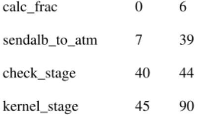
described by a set of configuration files that are manually defined by us. Figure 7 shows a part of the runtime configu-ration file of the algorithm list for the coupler component. In detail, each line is the keyword of a runtime algorithm. The first column in the keyword specifies the type of the runtime algorithm.Transferdenotes a data transfer algorithm,remap denotes a data interpolation algorithm, andnormaldenotes an external algorithm. The second column specifies the con-figuration file of the runtime algorithm. In sum, this runtime configuration file clearly lists out 91 runtime algorithms. For each runtime algorithm, there are configuration files to spec-ify the input and output field instances.
calc_frac 0 6 sendalb_to_atm 7 39 check_stage 40 44 kernel_stage 45 90
Figure 8.The runtime configuration file of the runtime procedures for the coupler component in FGOALS-gc.
list in Fig. 7. Then a runtime procedure can find the keywords of all runtime algorithms in it.
Our tests show that FGOALS-gc achieves the same (bitwise-identical) simulation result with FGOALS-g2. This result demonstrates that C-Coupler1 can be used to construct a coupler component for a complicated coupled model, such as a CSM, without changing the simulation result. FGOALS-g2 and FGOALS-gc can be downloaded through “svn–username=guest–password=guest co http://thucpl1. 3322.org/svn/coupler/CCPL_CPL6_consistency_checking.”
When constructing the experiment models GAMIL2-CLM3 and MASNUM-POM, we did not build a separate coupler component but used the direct coupling where no separate executable is generated for coupling. For GAMIL2-CLM3, as GAMIL2 and CLM3 share the same horizon-tal grid, there is only data transfer between them. For MASNUM-POM, as the grid of MASNUM is different from the grid of POM, both data transfer and data interpolation are between these two component models.
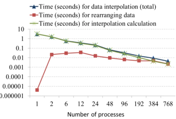
5.2 Parallel 3-D coupling
In MASNUM-POM, there is only one coupling field, the wave-induced mixing coefficient (Qiao et al., 2004), a 3-D field from MASNUM to POM. As the horizontal grids and vertical grids in these two component models are different, 3-D interpolation is required during coupling. In detail, we use CoR to generate the remapping weights for the 3-D in-terpolation. The corresponding 3-D remapping algorithm is generated through cascading two remapping algorithms: a bi-linear remapping algorithm for the horizontal grids and a 1-D spline remapping algorithm for the vertical grids. For the 1-D vertical interpolation, MASNUM and POM have different kinds of vertical grids: azgrid for MASNUM and asigma grid for POM.
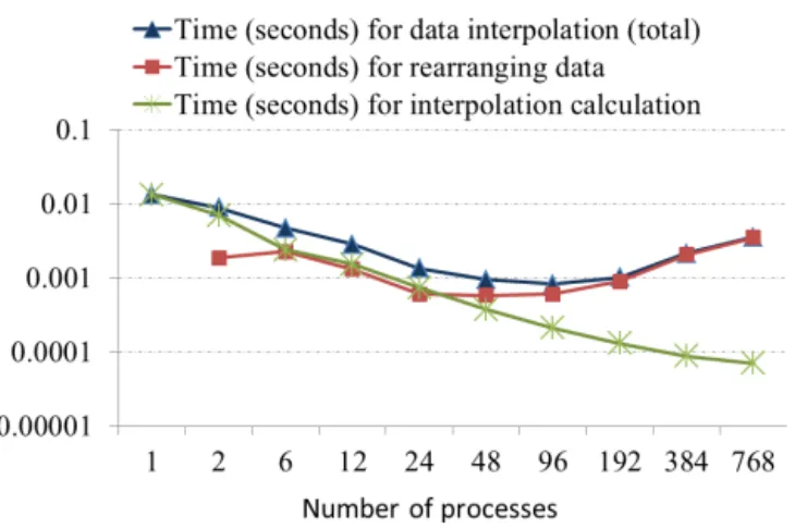
As introduced in Sect. 5.1, MASNUM-POM uses direct coupling without a coupler component. As the resolution of MASNUM is lower than the resolution of POM, we put the calculation of the 3-D interpolation in the runtime proce-dure of POM in order to achieve better parallel performance. Therefore, the 3-D interpolation shares the same processes with POM. When POM runs with multiple processes, the 3-D interpolation is computed in parallel. Our evaluation shows
that the 3-D interpolation keeps the same (bitwise-identical) result with different numbers of processes.
5.3 Code sharing
The experiment models FGOALS-gc, GAMIL2-CLM3, and GAMIL2-sole share the same atmosphere model, GAMIL2. In FGOALS-gc, the surface fields required by GAMIL2 are provided by other component models and computed by the coupler component with C-Coupler1. In GAMIL2-CLM3, the surface fields required by GAMIL2 are provided by CLM3 and the I/O data files which contain ocean fields and sea ice fields, and computed by the private flux algorithms in GAMIL2. GAMIL2-sole is similar to GAMIL2-CLM3, while the difference is that GAMIL2-sole directly calls a land surface package to simulate the surface fields from the land. Therefore, in these three experiment models, GAMIL2 has different procedures for the surface fields.
However, we make GAMIL2 share the same code version in these three experiment models. All algorithms for com-puting the input surface fields in GAMIL2 have been reg-istered to C-Coupler1 as the private external algorithms. In different experiment models, the same runtime procedures of GAMIL2 have different lists of runtime algorithms. As a result, all these experiment models keep the same (bitwise-identical) simulation result with the original model versions without C-Coupler1.
MASNUM-POM and MASNUM-sole share the same wave model, MASNUM, while MASNUM-POM and POM-sole share the same ocean model, POM. Similarly, we make MASNUM and POM share the same code in these exper-iment models that keeps the same (bitwise-identical) sim-ulation result with the original model versions without C-Coupler1.
5.4 Parallel performance
To evaluate the parallel performance of C-Coupler1, we use a high-performance computer named Tansuo100 in Tsing-hua University in China. It consists of more than 700 com-puting nodes, each of which contains two Intel Xeon 5670 six-core CPUs and 32 GB main memory. All computing nodes are connected by a high-speed InfiniBand network with peak communication bandwidth 5 GB s−1. We use the
Intel C/C++/Fortran compiler version 11.1 and the Intel MPI library version 4.0 for compiling the experiment mod-els, with optimization level O2 or O3.