Geosci. Model Dev., 9, 1853–1890, 2016 www.geosci-model-dev.net/9/1853/2016/ doi:10.5194/gmd-9-1853-2016
© Author(s) 2016. CC Attribution 3.0 License.
Representation of the Community Earth System Model (CESM1)
CAM4-chem within the Chemistry-Climate Model Initiative
(CCMI)
Simone Tilmes1, Jean-Francois Lamarque1, Louisa K. Emmons1, Doug E. Kinnison1, Dan Marsh1, Rolando R. Garcia1, Anne K. Smith1, Ryan R. Neely1, Andrew Conley1, Francis Vitt1, Maria Val Martin2, Hiroshi Tanimoto3, Isobel Simpson4, Don R. Blake4, and Nicola Blake4
1National Center for Atmospheric Research, Boulder, CO, USA 2The University of Sheffield, Sheffield, S1 3JD, UK
3National Institute for Environmental Studies, Tsukuba, Ibaraki 305-8506, Japan 4University of California, Irvine, CA, USA
Correspondence to:Simone Tilmes ([email protected])
Received: 23 October 2015 – Published in Geosci. Model Dev. Discuss.: 18 January 2016 Revised: 8 April 2016 – Accepted: 21 April 2016 – Published: 20 May 2016
Abstract. The Community Earth System Model (CESM1) CAM4-chem has been used to perform the Chemistry Cli-mate Model Initiative (CCMI) reference and sensitivity sim-ulations. In this model, the Community Atmospheric Model version 4 (CAM4) is fully coupled to tropospheric and strato-spheric chemistry. Details and specifics of each configu-ration, including new developments and improvements are described. CESM1 CAM4-chem is a low-top model that reaches up to approximately 40 km and uses a horizontal resolution of 1.9◦latitude and 2.5◦longitude. For the speci-fied dynamics experiments, the model is nudged to Modern-Era Retrospective Analysis for Research and Applications (MERRA) reanalysis. We summarize the performance of the three reference simulations suggested by CCMI, with a fo-cus on the last 15 years of the simulation when most ob-servations are available. Comparisons with selected data sets are employed to demonstrate the general performance of the model. We highlight new data sets that are suited for multi-model evaluation studies. Most important improvements of the model are the treatment of stratospheric aerosols and the corresponding adjustments for radiation and optics, the updated chemistry scheme including improved polar chem-istry and stratospheric dynamics and improved dry deposi-tion rates. These updates lead to a very good representa-tion of tropospheric ozone within 20 % of values from avail-able observations for most regions. In particular, the trend and magnitude of surface ozone is much improved
com-pared to earlier versions of the model. Furthermore, strato-spheric column ozone of the Southern Hemisphere in winter and spring is reasonably well represented. All experiments still underestimate CO most significantly in Northern Hemi-sphere spring and show a significant underestimation of hy-drocarbons based on surface observations.
1 Introduction
comparison studies. Improvements in comparison to earlier versions of the model are discussed in the Conclusions.
2 Model description
CESM is a fully coupled Earth System model, which in-cludes atmosphere, land, ocean and sea-ice components. All CCMI simulations are carried out with the same model code that is based on CESM version 1.1.1 (CESM1) (Neale et al., 2013), with modifications discussed below. The configura-tion of the model used here fully couples the Community At-mosphere Model version 4 (CAM4), the Community Land model version 4.0 (CLM4.0), the Parallel Ocean Program version 2 (POP2) and the Los Alamos sea ice model (CICE version 4). The land model was run without an interactive carbon or nitrogen cycle and only the atmospheric and land components are coupled to the chemistry. The climatological present-day land cover is used for all simulations.
2.1 The atmosphere model
Detailed information about the physics of the atmosphere model used here are described in Neale et al. (2013) and Richter and Rasch (2008), and also summarized in Lamarque et al. (2012, and references therein). In summary, deep con-vection is treated by Zhang and McFarlanle (1995) with im-provements in the convective momentum transport (Richter and Rasch, 2008), which improved surface winds, stresses and tropical convection. At the same time, an entraining plume was added to the convection parameterization, which together with the momentum transport improved the repre-sentation of El Niño–Southern Oscillation (ENSO) signifi-cantly (Neale et al., 2008). The photolysis calculation uses a look-up table between 200 and 750 nm and online calcula-tions for wavelengths<200 nm. Only changes in the ozone column, but not in the aerosol burden, impact photolysis rates. Attenuation of the spectral irradiance above the model top is calculated using the approach of Kinnison et al. (2007) and Lamarque et al. (2012).
due to differences in the meteorology to ensure values of ap-proximately 3–5 Tg N year−1for present-day conditions. 2.1.1 Model grid
For all CCMI reference simulations, CESM1 CAM4-chem uses a horizontal grid with a resolution of 1.9◦×2.5◦ (lat-itude by long(lat-itude), and uses the finite volume dynami-cal core. The top of the model is located at 3 hPa (about 40 km). The vertical coordinate is sigma (hybrid terrain-following pressure) in the troposphere, switching over to iso-baric at pressure levels less than 100 hPa; the vertical res-olution of the model depends on the configuration of the experiment. The atmosphere model, CAM4, makes use of two different configurations, the FR (with 26 vertical levels) and the SD(with 56 vertical levels adopted from the analy-sis fields); see Lamarque et al. (2012). For the SD config-uration, internally derived meteorological fields are nudged every time step of 30 min by 1 % towards reanalysis fields (equivalent to a 50 h Newtonian relaxation timescale for nudging) from Modern-Era Retrospective Analysis for Re-search and Applications (MERRA) reanalysis (http://gmao. gsfc.nasa.gov/merra/) (Rienecker et al., 2011). Nudged me-teorological fields include wind components, temperatures, surface pressure, surface stress, latent and sensible heat flux. The MERRA reanalysis fields are interpolated to the hori-zontal resolution of the model prior to running the simula-tion. The MERRA surface geopotential height is used for the SD simulations to be consistent with the reanalysis fields. 2.1.2 Quasi-Biennial Oscillation
S. Tilmes et al.: Representation of CESM1 CAM4-chem within CCMI 1855 vary the QBO phase between eastward and westward phase
using an approximate 28-month period, similar to what was done by Marsh et al. (2013).
2.1.3 Improved gravity wave representation
The representation of sub-grid-scale gravity waves (GW) in CAM was formerly limited to orographic gravity waves us-ing the parameterization adapted from McFarlane (1987). In the present simulations, the parameterizations of non-orographic gravity waves generated by convection (Beres et al., 2005) and fronts (Richter et al., 2010), which were developed for the Whole Atmosphere Community Climate Model (WACCM), are also included.
In addition, we have added another gravity wave mod-ule to represent the waves with large horizontal wavelengths that are often observed in the stratosphere (e.g., Zink and Vincent, 2001). The new GW module is adopted from the inertia-gravity wave (IGW) parameterization developed by Xue et al. (2012) for an interactive QBO. The formulation includes the impact of the Coriolis force on gravity wave propagation and breaking. Rather than applying it in the equatorial region, as done by Xue et al. (2012), we use a more general mechanism for determining sources; gravity waves are triggered by the same frontal threshold used for the mesoscale gravity waves (Richter et al., 2010). This has the impact of shifting the bulk of the waves from the tropics to middle and high latitudes. In the current implementation, gravity waves have a narrow phase speed spectrum (−20 to 20 m s−1) and long horizontal wavelength (1000 km). The momentum forcing associated with this module particularly impacts the winter stratosphere. In the Southern Hemisphere (SH), it enhances downwelling and increases the winter stratospheric temperature, which in previous simulations was substantially colder than observed.
However, it was found, that the version of the IGW param-eterization used for the performed experiments has a narrow IGW spectrum centered on zero phase velocity instead of be-ing centered on the speed of the background wind at the GW launch level, as in the standard GW parameterization. Even with this shortcoming, the model produces a much improved temperature evolution in the stratosphere, in particular in the SH high latitudes compared to earlier versions. This results in a well-resolved ozone hole in winter and spring over Antarc-tica. No significant changes are expected from a corrected IGW parameterization for the troposphere.
2.1.4 Tropospheric aerosols
CAM4-chem runs with the bulk aerosol model (BAM), which simulates the distribution of externally mixed sulfate, black carbon (BC), primary organic carbon (OC), sea-salt and dust, as described in Lamarque et al. (2012). The dust emissions are calibrated so that the global dust aerosol opti-cal depth (AOD) is about 0.025 to 0.030 (Mahowald et al.,
2006). The distribution of sea-salt and dust are described using four size bins. In CAM4-chem, the formation of sec-ondary organic aerosols (SOA) is coupled to the chemistry and biogenic emissions. SOA are derived using the two-product model approach using laboratory determined yields for SOA formation from monoterpene, isoprene and aromatic photooxidation, as described in Heald et al. (2008). The ag-ing process of BC and OC from hydrophobic to hydrophilic is included through a specified conversion timescale. For all aerosol species, the size distributions are specified as in Lamarque et al. (2012). Aerosols interact with the gas-phase chemistry through heterogeneous reactions that depend on the available surface area density (SAD), as discussed below. For the tropospheric SAD calculation, sulfate, hydrophilic black carbon, primary organic carbon and nitrates are in-cluded, where SOA has not been included. This may lead to a significant underestimation of tropospheric SAD in the experiments.
2.1.5 Representation of aerosols in the stratosphere Aerosol mass, heating rates and SAD are revised in this ver-sion compared to earlier configurations. Most significantly, the model uses a new stratospheric aerosol and SAD data set, derived based on observations, to force models partici-pating in CCMI (Eyring et al., 2013). In addition, in order to fully utilize the aerosol size information provided by the new model input file, the optics in the radiative transfer code as-sociated with CAM4 (i.e., CAMRT) (Neale et al., 2010) have been modified to include a lookup table for aerosol effective radius in the shortwave radiation scheme. The new descrip-tion leads to an updated representadescrip-tion of volcanic heating for REFC1 and REFC2, whereas in REFC1SD volcanic heating is included through the nudged temperature fields. See Neely et al. (2015) for a full description of changes to the strato-spheric aerosol scheme. Tropostrato-spheric aerosols that enter the stratosphere are promptly removed (as listed in Table A2) since the aerosol burden in the stratosphere is prescribed. 2.1.6 Coupling to the land model
Dry deposition velocity for tracers in the atmosphere are cal-culated online in CLM4.0. An updated calculation is used, where leaf and stomatal resistances are coupled to the leaf area index (LAI) and are also linked to the photosynthesis provided by the land model, as described in Val Martin et al. (2014).
boundary conditions, as indicated in Table A1, as discussed in Sect. 2.3.2. Different species experience wet and/or dry deposition, as also listed in Table A1. Furthermore, 14 artificial tracers are implemented as recommended by CCMI (Eyring et al., 2013, Sect. 4.2.1): NH5, NH50, NH50W, AOANH, ST8025, CO25, CO50, SO2t, SF6em, O3S, E90, E90NH, E90SH. O3S is a stratospheric ozone tracer that represents the amount of ozone in the troposphere with its source in the stratosphere. O3S is set to stratospheric values at the tropopause, and experiences the same loss rates as ozone in the troposphere, as defined by CCMI. As interpreted from the CCMI recommendation, dry deposition is not included, which will lead to an overestimation of O3S in the lower boundary layer when compared to ozone (which is dry deposited).
The chemical mechanism, is based on the Model for Ozone and Related chemical Tracers (MOZART), version 4 mechanism for the troposphere (Emmons et al., 2010). It further includes extended stratospheric chemistry (Kinnison et al., 2007) and updates, as described in Lamarque et al. (2012) and Tilmes et al. (2015). The reactions include pho-tolysis, gas-phase chemistry and heterogeneous chemistry, in both troposphere and stratosphere. The complete chemi-cal mechanism is listed in Table A2 and incorporates all the latest updates. All aerosols and some gas-phase species, in-cluding H2O, O2, CO2, O3, N2O, CH4, CFC11, CFC12, are radiatively active.
Reaction rates are updated following JPL2010 recommen-dations (Sander et al., 2011). Bromoform (CHBr3) and di-bromomethane (CH2Br2) were added to the model to repre-sent the stratospheric bromine loading from very short-lived (VSL) species. The surface volume mixing ratio for these two VSL species was set globally to 1.2 ppt (i.e., 6 ppt total bromine). This approach adds an additional≈5 ppt of inor-ganic bromine to the stratosphere. The resulting stratospheric total inorganic bromine abundance (for present-day condi-tions) from both long-lived and VSL species is ≈21.5 ppt. Besides the current lower boundary condition (LBC) ap-proach for VSL species, CAM4-chem can be also config-ured with a full-VSL mechanism, including detailed gas-phase halogen chemistry mechanism, geographically and
O3-Prod=r(NO−HO2)+r(CH3O2−NO)
+r(PO2−NO)+r(CH3CO3−NO)
+r(C2H5O2−NO)+0.92·r(ISOPO2−NO)
+r(MACRO2−NOa)+r(MCO3−NO)
+r(C3H7O2−NO)+r(RO2−NO)
+r(XO2−NO)+0.9·r(TOLO2−NO)
+r(TERPO2−NO)+0.9·r(ALKO2−NO)
+r(ENEO2−NO)+r(EO2−NO)
+r(MEKO2−NO)+0.4·r(ONITR−OH)
+jonitr
O3-Loss=r(O1D−H2O)+r(OH−O3)
+r(HO2−O3)+r(C3H6−O3)
+0.9·r(ISOP−O3)+r(C2H4−O3)
+0.8·r(MVK−O3)+0.8·r(MACR−O3)
+r(C10H16−O3).
These are defined based on the rate-limiting terms for the gas-phase reactions of the Oxfamily (O3, O, O1D , NO2), not including O2+hv→2O production, Ox, ClOx, and BrOx
losses, and are therefore not valid for the stratosphere. The sum of those rates are very similar to the explicit calculation of the net chemical change of ozone (as listed in Table A2). 2.3 Experimental Setup
ev-S. Tilmes et al.: Representation of CESM1 CAM4-chem within CCMI 1857 ery 5–10 years. All emissions include a seasonal cycle.
Bio-genic emissions are calculated every time step by MEGAN, as described in Sect. 2.1.6.
The REFC1SD experiment is nudged to analyzed air tem-peratures, winds, surface fluxes and surface pressure, and uses the Hadley Centre Global Sea Ice and Sea Surface Temperature version 2 (HadISST2) observed time-dependent data set for sea surface temperatures (SSTs) and sea ice. The REFC1 experiment also uses prescribed SSTs and sea ice, while the REFC2 simulation calculates temperatures in the ocean and atmosphere. We have carried out one simulation for REFC1SD, and an ensemble of three members for each REFC1 and REFC2.
The solar cycle is prescribed using observed daily fields for the years until 2010. For the future period in REFC2, we follow the CCMI recommendation and repeat a sequence of the last four solar cycles (20–23), as defined in http: //solarisheppa.geomar.de/ccmi.
2.3.1 Initial conditions and spin-up
CAM4-chem initial conditions for the three REFC1 and REFC2 ensemble members are taken from 3 realizations of CESM1-WACCM 20th Century ensemble for CMIP5 (Marsh et al., 2013). The spin-up period started in 1950 and ran through 1959. The experiments simulated the years 1960 to 2010 (REFC1) and 1960 to 2100 (REFC2). Initial condi-tions for the REFC1SD simulation are taken from the first REFC1 ensemble member in 1975. The spin-up of this ex-periment covered the years 1975 to 1979, repeating 1979 meteorological analysis for each year. The experiment was performed between 1980 and 2010.
2.3.2 Lower boundary conditions
For all of the three reference experiments the same monthly and annually varying lower boundary conditions are used based on the Representation Concentration Pathway 6.0 (RCP6.0) Coupled Model Intercomparison Project Phase 5 (CMIP5) future projection (Taylor et al., 2012). We prescribe CO2, N2O, CH4, as well as the following halogen species based on the CCMI recommendations: CCl4, CF2ClBr, CF3Br, CFC11, CFC113, CFC12, CH3Br, CH3CCl3, CH3Cl, H2, HCFC22, CFC114, CFC115, HCFC141b, HCFC142b, CH2Br2, CHBr3, H1202, H2402, SF6. A north–south gradient was added for CH3Br, HCFC22, HCFC141b, HCFC142b, based on the HIAPER (High-Performance In-strumented Airborne Platform for Environmental Research) Pole-to-Pole Observations (HIPPO) (Wofsy et al., 2011; Mi-jeong Park, personal communication, 2015).
3 Model performance 3.1 Global diagnostics
The general state of the model is investigated by compar-ing diagnostics of globally averaged values between different model experiments that are averaged between 1995 and 2010 (Table 1). The global surface temperatures (TS) of all three experiments are in agreement within 0.15 K for the observed period (Table 1). REFC1SD land temperature (TS land) is on average 0.25 K higher than for REFC1 and 0.15 K higher than for the REFC2 experiments (Table 1). The largest devia-tions occur over high latitudes (not shown). In the REFC1SD experiment, low cloud fraction is significantly larger than in the other experiments, which results in a much smaller short-wave cloud forcing (SWCF) of−83 W m−2 compared the other experiments that are with 54–56 W m−2 more in line with observations.
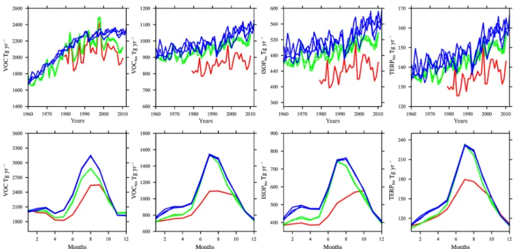
Differences in clouds and land surface temperatures be-tween the reference experiments result in different biogenic emissions of volatile organic components (VOCs) (Fig. 1). REFC1SD biogenic emissions are about 10 % lower than in the REFC1 experiment and about 15 % lower than in the REFC2 experiment. The emissions differ the most in sum-mer during their peak (Fig. 1, bottom row). Despite the fact that surface temperatures in REFC1SD are warmer than in REFC1, more low cloud clouds and reduced solar radia-tion (as evident in photolysis rates) near the surface may be the important driver for the reduced biogenic emissions in REFC1SD, which has to be further investigated. Other dif-ferences in the REFC1 and REFC2 VOC emissions arise from different anthropogenic and biomass burning emis-sions, while biogenic emissions differ by less than 10 % (Ta-ble 1). Despite the variation in the reference experiments, biogenic emissions are in agreement with earlier estimates (e.g., Young et al., 2013).
CH4Lifet. (year) 7.6 8.0 8.1 8.1 8.2 8.2 8.2
CH3CCl3Lifet. (year) 4.5 4.8 4.8 4.8 4.9 4.9 4.9
CO Burden (Tg) 289.6 303.6 305.3 305.7 315.4 316.7 315.3 CO Emis. (Tg year−1) 1114.8 1119.3 1126.5 1126.8 1170.1 1171.1 1169.9 CO Dep. (Tg year−1) 125.8 120.7 122.0 122.1 122.7 123.0 122.9 CO Chem. Loss (Tg year−1) 2264.1 2294.2 2295.3 2298.0 2348.4 2353.3 2345.5
CO Lifet. (days) 44.2 45.9 46.1 46.1 46.6 46.7 46.6
O3Burden (Tg) 332.5 326.9 326.5 326.4 327.8 327.2 327.0 O3Dep. (Tg year−1) 871.7 894.4 893.9 894.2 895.0 892.8 894.7 O3Chem. Loss (Tg year−1) 4256.0 4268.3 4250.6 4259.0 4287.6 4293.5 4278.9 O3Chem. Prod. (Tg year−1) 4693.8 4710.0 4706.5 4708.3 4747.2 4756.9 4744.1 O3Net Chem.Change (Tg year−1) 392.9 420.9 430.5 426.0 432.5 436.5 438.2 O3STE (Tg year−1) 478.8 473.4 463.4 468.2 462.5 456.4 456.5
Isop. Emis. (Tg year−1) 454.2 512.6 511.8 515.0 546.6 551.6 545.6 Monoterp. Emis. (Tg year−1) 138.9 150.0 150.0 150.3 155.4 156.4 155.0 Methanol Emis. (Tg year−1) 100.4 114.6 114.8 114.9 113.7 114.9 113.4 Aceton Emis. (Tg year−1) 41.6 44.3 44.3 44.3 47.8 48.1 47.7
Lightning Prod. (TgN year−1) 4.5 4.8 4.7 4.8 4.7 4.7 4.7
Total optical depth 0.107 0.119 0.119 0.119 0.118 0.118 0.118 Dust optical depth 0.041 0.043 0.043 0.043 0.040 0.041 0.040
POM Burden (TgC) 0.75 0.73 0.73 0.74 0.77 0.77 0.77
POM Emis. (TgC year−1) 48.38 47.99 48.38 48.38 51.23 51.23 51.23
POM Lifet. (days) 7.23 7.18 7.15 7.19 7.05 7.06 7.01
SOA Burden (TgC) 0.54 0.49 0.49 0.49 0.51 0.51 0.50
SOA Chem. Prod. (TgC year−1) 32.79 34.45 34.43 34.79 35.86 36.32 35.54
SOA Lifet. (days) 0.54 0.49 0.49 0.49 0.51 0.51 0.50
BC Burden (TgC) 0.12 0.12 0.12 0.12 0.12 0.12 0.12
BC Emis. (TgC year−1) 7.71 7.68 7.71 7.71 7.95 7.95 7.95
BC Lifet. (days) 7.44 7.48 7.46 7.49 5.88 5.89 5.86
DUST Burden (TgC) 43.87 45.04 45.03 45.20 42.60 42.75 42.31 SALT Burden (TgC) 6.02 10.88 10.88 10.87 11.14 11.10 11.11
SO4Burden (TgS) 0.45 0.49 0.49 0.49 0.51 0.51 0.51
SO4Emis. (TgS year−1) 0.25 0.25 0.25 0.25 0.25 0.25 0.25 SO4Dry Dep. (TgS year−1) 5.29 5.76 5.78 5.77 5.94 6.00 5.99 SO4Wet Dep. (TgS year−1) −49.93 −46.36 −46.28 −46.30 −46.36 −46.42 −46.49 SO4Chem. Prod. (TgS year−1) 10.35 10.81 10.83 10.82 10.98 11.02 11.02 SO4AQ. Prod. (TgS year−1) 44.95 41.41 41.34 41.35 41.44 41.53 41.58 SO4Total Prod. (TgS year−1) 55.30 52.23 52.17 52.18 52.42 52.55 52.60
S. Tilmes et al.: Representation of CESM1 CAM4-chem within CCMI 1859
Figure 1.Global-averaged surface emissions of total volatile organic compounds (VOCs) (first column), biogenic VOCs (second column), biogenic isoprene (third column), and biogenic terpenes (fourth column), for different experiments, REFC1SD (red), REFC1 (green), REFC2 (blue). The seasonal cycle of zonal averages between 1960 and 2010 are shown at the bottom row.
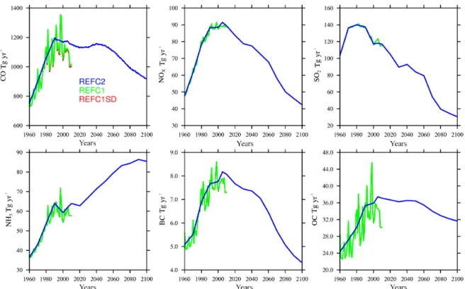
3.2 Trends of tropospheric components
Time-varying emissions of ozone precursors and aerosols impact the oxidation capacity of the atmosphere. In the following, we discuss the evolution of different chemical species and surface area density in the tropical troposphere between 30◦S and 30◦N, tropospheric methane lifetime and stratospheric column ozone (Fig. 2), since methane is mostly controlled by processes in the tropics. Increasing ni-trogen dioxide (NO2), CO and VOC burdens between 1960 and 1990 result in increasing tropospheric ozone with the strongest trend between 1960 and 1990. Increasing aerosols between 1960 and 1990 result in an increase in SAD, with little change after 1990. Together with the increase in CO burden, this results in a decrease of OH. Other factors re-sult in an increase in tropospheric OH, including decreasing stratospheric column ozone between 1960 and 2010, increas-ing tropospheric column ozone, increasincreas-ing nitrogen dioxides (NOx) burden, and decreasing methane emissions (e.g.,
Mur-ray et al., 2014). Both counteracting effects on OH result in little change in methane lifetime between 1960 and 1990. Af-ter 1990, SAD, as well as CO and VOC, trends are leveling off, but nitrogen dioxide and ozone burdens are still increas-ing, partly due to increasing lightning NOxproduction (not
shown). This results in a decreasing trend in methane lifetime after 1990 for all reference experiments.
The burden of chemical tracers differs between REFC1SD and REFC1/REFC2 (Fig. 2). Variations in emissions and at-mospheric dynamics, including surface temperature, clouds and convection, influence the chemical composition of the
atmosphere. Exchange processes between the upper tro-posphere and lower stratosphere are also different in the model experiments and impact ozone. The shorter lifetime of methane in REFC1SD compared to the other experiments may be a result of a reduction in high clouds, and, to some amount, the larger ozone mixing ratios in the tropical tropo-sphere, which would increase the oxidation capacity in the tropics. This has to be investigated in more detail in future studies.
Besides a continuous decrease, the stratospheric ozone column shows a significant drop after major volcanic erup-tions (e.g., WMO, 2006). This is expected due to an increase in stratospheric SAD after the eruption, which causes en-hanced halogen activation, resulting in ozone depletion (see Fig. 2).
4 Evaluation against selected diagnostics
Figure 2.Time series of annually averaged column integrated tropospheric and tropical nitrogen dioxide (in Tg N), tropospheric ozone burden, and CO, in (30◦S–30◦N), tropical average of tropospheric surface area density, global stratospheric column ozone and tropospheric methane lifetime.
4.1 Ozone
Ozone is an important atmospheric tracer in both the tropo-sphere and the stratotropo-sphere. In the tropotropo-sphere and at the surface, ozone is an air pollutant and is impacted by vari-ous precursors, most importantly CO and NOx. A
reason-able performance of tropospheric ozone is required for air quality studies. In the stratosphere, ozone is strongly influ-enced by dynamics, photo-chemistry and catalytic reactions (e.g., WMO, 2011). The strength of the transport of strato-spheric ozone into the troposphere follows a seasonal cycle controlled by the Brewer–Dobson circulation (BDC). Short-comings in the representation of the strength of the BDC and mixing processes between stratosphere and troposphere in-fluence the performance of tropospheric ozone, as discussed below. In addition, ozone is an important greenhouse gas in the upper troposphere and lower stratosphere (UTLS) and in-fluences tropospheric climate (e.g., WMO, 2014).
4.1.1 Trends and seasonality of ozone
Ozone trends and seasonality in the reference experiments are compared to ozonesonde observations (Tilmes et al., 2012) in the free troposphere (at 500 hPa) and the bound-ary layer (at 900 hPa). For Japan, we employ an additional climatology derived by Tanimoto et al. (2015), which is based on surface observations at five marine boundary layer
sites from the Acid Deposition Monitoring Network in East Asia (EANET) for pressure levels larger than 900 hPa, and a combination of the historical Measurements of OZone, water vapor, carbon monoxide and nitrogen oxides by in-service AIrbus airCraft (MOZAIC; URL: http://www.iagos. fr/mozaic) data (over Narita airport) and ozonesonde obser-vations (at Tateno/Tsukuba) for pressure levels between 472 and 616 hPa. We use an artificial stratospheric ozone tracer (O3S) to identify differences in stratosphere–troposphere ex-change (STE) between different model experiments for four selected regions (see Figs. 3 and 4).
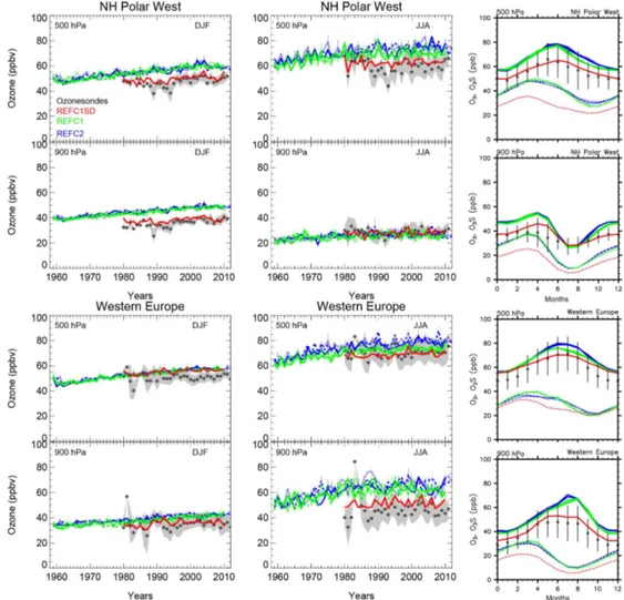
In high northern latitudes, REFC1SD reproduces the mag-nitude and trend of ozone very well, including variability within the standard deviation of the observations for all sea-sons, as shown in the example of the Northern Hemisphere (NH) polar west region (Fig. 3, first and second row). A very good agreement between the model experiment and ozonesondes also exists for western Europe, with the ex-ception of the high bias between October and February at 500 hPa of 5–10 ppb (Fig. 3, third and fourth row).
ex-S. Tilmes et al.: Representation of CESM1 CAM4-chem within CCMI 1861
Figure 3.Left and middle column: time evolution of seasonal averaged and regionally aggregated ozone mixing ratios derived from ozone soundings (black diamonds) and model results (colored lines) at two different pressure levels, two different seasons (DJF: left, JJA: right) and regions (NH polar west, and western Europe). Grey shading indicates the standard deviation of the observations that include at least 12 observed profiles per season in a year. Colored error bars indicate the standard deviation based on monthly averaged model output. Right column: Regionally aggregated seasonal cycle comparisons of ozone soundings (black lines) and model simulations (colored lines), averaged between 1995 and 2010. Dashed lines indicate mixing ratios of the stratospheric ozone tracer (see text for more details).
plained by differences in O3S for the whole year at 500 hPa and for winter months at 900 hPa. During summer months, differences in chemical production at the surface for the dif-ferent experiments seem to play an additional role and ex-plain about 5–10 ppb of the deviations for western Europe.
Selected ozonesondes over eastern USA and Japan are lo-cated further south and are more strongly influenced by trop-ical air masses and tropospheric intrusion in the lowermost stratosphere in particular in winter, as discussed in Tilmes et al. (2012). Each of the regions covers only two stations and so uses fewer observations for the different years than other regions, which increases the uncertainty of trends (Saunois et al., 2012).
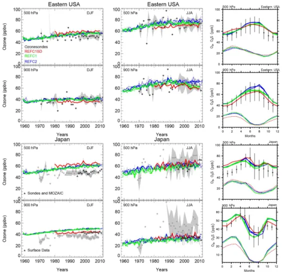
Comparisons for eastern USA and Japan are illustrated in Fig. 4. For Japan, we are using two data sets to compare to model results. Ozone mixing ratios and trends at 900 hPa over Japan using ozonesondes, as compiled by Tilmes et al.
(2012), Fig. 4 (black diamonds), largely differ from the cli-matology by Tanimoto et al. (2015), which is based on sur-face observations (black triangles). This is due to uncertain-ties in the ozonesonde observations at these altitudes, which should be treated with caution. On the other hand, the two climatologies agree well in the free troposphere at 500 hPa.
Figure 4.As Fig. 3, but for Eastern USA and Japan instead. For Japan, ozone time series compiled by Tanimoto et al. (2015) are added (black triangles) (see text for more details) and used to compare with the seasonal cycle of the model for Japan.
tracer (see Fig. 4). At 500 hPa, ozone mixing ratios and trends are well reproduced for all experiments in summer. However, the model overestimates winter ozone mixing ra-tios in the upper troposphere.
4.1.2 Present-day ozone
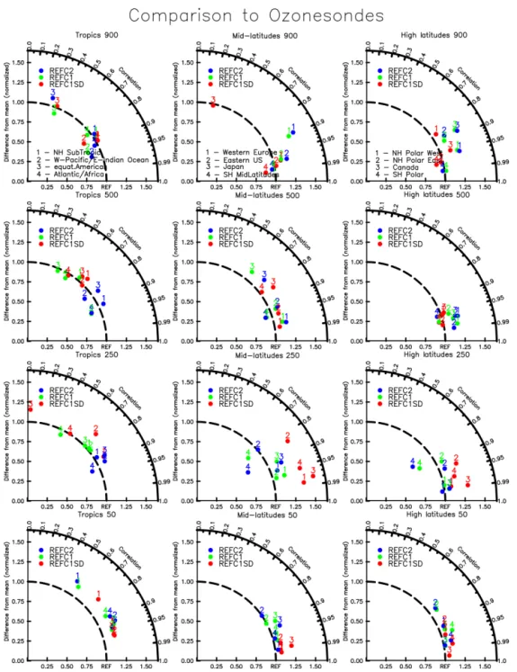
A comparison with ozonesonde observations over different regions for simulated years between 1995 and 2010 is pre-sented in Fig. 5. Besides some differences in ozone compared to observations, as discussed above, all model experiments reproduce observed tropospheric ozone within 25 % for most of the regions. At 250 hPa, which is the UTLS at mid- and high latitudes, REFC1SD overestimates ozone by up to 50 %, particularly at mid-latitudes in both hemispheres. This could be the result of strong mixing in the UTLS associated with the use of the small nudging amount of 1 % in this study; however, this needs to be investigated in more detail in fu-ture studies. The other experiments show smaller deviations from the observations of about 20 % or less. Tropical values at 50 hPa are overestimated by no more than 20 % compared
to observations for all the experiments, while ozone in the mid- and high latitudes in the stratosphere agrees within 10 % with observations.
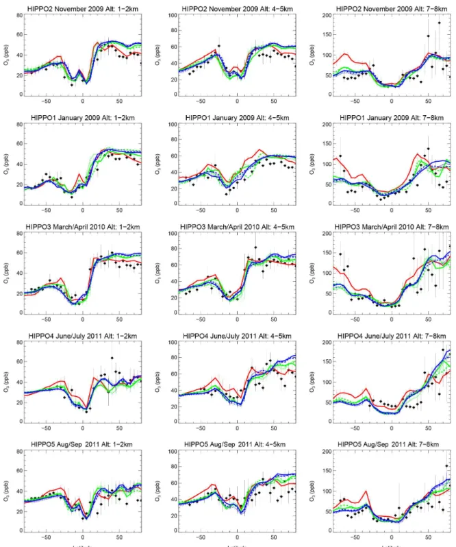
Model results further agree well with HIPPO aircraft ob-servations for profiles sampled from 85◦N to 65◦S over the Pacific Ocean between 2009 and 2011 (Fig. A2). In REFC1SD, lower troposphere values (1–2 km) are within the range of the observations, while for REFC1 and REFC2 ozone is overestimated by about 5 ppb in high northern lat-itudes, in particular in winter and spring, which points to a transport problem as discussed above. Some differences, especially at higher altitudes (7–8 km) are likely caused by the specific meteorological situation for the flight conditions compared to the climatological model results.
S. Tilmes et al.: Representation of CESM1 CAM4-chem within CCMI 1863
Figure 5. Taylor-like diagram comparing the mean and correlation of the seasonal cycle between observations using a present-day ozonesonde climatology between 1995 and 2011 and model results between 1995 and 2010, interpolated to the same locations as sam-pled by the observations and for different pressure levels, 900 hPa (top panel), 500 hPa (second panel), 250 hPa (third panel) and 50 hPa (bottom panel). Different numbers correspond to a specific region, as defined in Tilmes et al. (2012). Left panels: 1 – NH-subtropics; 2 – W-Pacific/eastern Indian Ocean; 3 – equat. Americas; 4 – Atlantic/Africa. Middle panels: 1 – western Europe; 2 – eastern USA; 3 – Japan; 4 – SH mid-latitudes. Right panels: 1 – NH polar west; 2 – NH polar east; 3 – Canada; 4 – SH polar.
(Kalabokas et al., 2013; Zanis et al., 2014), are reproduced by the REFC1 and REFC1SD experiments. The ozone gra-dient between mid-latitudes and tropics is for the most part well captured, for example over Japan in summer. The pole to mid-latitude ozone gradient in the SD simulation showed a larger southward ozone gradient than the REFC1
simula-tion, which is more consistent with the measurements. Re-gional differences in tropospheric ozone between the differ-ent model experimdiffer-ents have to be investigated in future stud-ies.
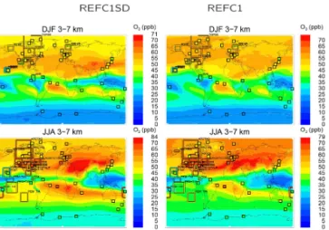
Monitor-Figure 6. Comparison between model results in contours (REFC1SD left and REFC1.1 right) and observations of ozone mix-ing ratios, averaged over 3–7 km for December–January–February (DJF), top, and June–July–August (JJA), bottom. The color of each square represents the value of the observed ozonesonde measure-ment for the same period and altitude interval, and the color of framed regions corresponds to values derived from aircraft obser-vations averaged over the particular region for each experiment (Tilmes et al., 2015).
ing Instrument (OMI) and Microwave Limb Sounder (MLS) satellite observations between 2004 and 2010, compiled by Ziemke et al. (2011), in the troposphere (Fig. 7) and strato-sphere (Fig. 8). The model tropopause for this diagnostic is defined as the 150 ppb ozone level, which may lead to small differences between observations and model simula-tions, but not between model experiments themselves. The comparisons reveal additional characteristics of the model performance compared to observations. Tropospheric col-umn ozone is reproduced within±10 DU of the observations, with a close agreement to the satellite climatology within less than±5 DU in low and mid-latitudes in spring and summer (Fig. 7). All model experiments show a low bias in mid-latitudes in the SH and high bias by 10–15 DU in the NH mid-latitudes in winter and fall. NH tropospheric ozone is in general large in the REFC1 and REFC2 simulations com-pared to the REFC1SD experiments, as discussed above.
Stratospheric ozone in all model experiments agree within ±30 DU in mid- and low latitudes compared to the satellite climatology (Fig. 8). Larger deviations from the observations occur in the NH mid- and high latitudes in winter and spring with a high bias of up to 60 DU. Ozone in the SH is within about 25 DU from the observations and is reasonably well reproduced by all model experiments, especially for the free-running experiments.
4.2 Carbon monoxide
Carbon monoxide, non-methane hydrocarbons and nitrogen dioxides are the most important precursors to the formation
Figure 7.Monthly and zonally averaged tropospheric ozone col-umn (in DU) comparison between OMI/MLS observations (black) and different model experiments; see legend (for ozone<150 ppb in the model) for 4 months. Error bars describe the zonally aver-aged 2 sigma 6-year root mean square standard error of the mean at a giving grid point, derived from the 10◦N to 10◦S gridded prod-uct (Ziemke et al., 2011). Model results are interpolated to the same grid and error bars indicate the standard deviation of the interannual variability per latitude interval.
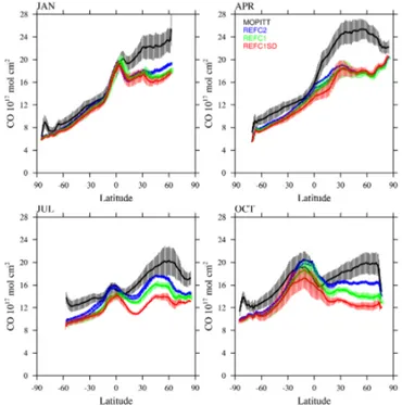
of tropospheric ozone. Carbon monoxide also impacts the oxidation capacity of the atmosphere and therefore methane lifetime. We compare the CO burden from different experi-ments to monthly and zonally averaged tropospheric column carbon monoxide derived from Measurements of Pollution in the Troposphere (MOPITT) version 6 level 3 satellite ob-servations, as described in Tilmes et al. (2015) (see Fig. 9). The climatological averaging kernel and a priori is applied to both observations and model experiments in the same way.
ex-S. Tilmes et al.: Representation of CESM1 CAM4-chem within CCMI 1865
Figure 8. As Fig. 7, but showing monthly and zonally averaged stratospheric ozone column comparison between OMI/MLS obser-vations (black) and different model experiments; see legend (for ozone>150 ppb in the model) for 4 months.
periments (not shown), which is consistent with more ozone in the tropical troposphere (see Fig. 2).
The simulated CO column in the tropics agrees with the satellite climatology within the interannual variability. How-ever, the model underestimates CO column in the SH for all the experiments, in particular in summer. In contrast, com-parisons to HIPPO CO in situ observations indicate very good agreement between CO mixing ratios in the SH over the remote region of the Pacific Ocean for most of the sea-sons (see Fig. A3). Furthermore, CO mixing ratios are largely underestimated in March and April in comparison to the air-craft observations, consistent with the satellite comparison. Differences in CO will be investigated in more detail in fu-ture studies.
4.3 Hydrocarbons
Hydrocarbons are important tropospheric compounds that are emitted from vegetation, biomass burning and anthro-pogenic sources, including oil and gas extraction activities. They are important ozone precursors, influence the oxidation capacity of the atmosphere, and eventually form CO.
Ethane and other hydrocarbons have been measured us-ing canister samples along coastal and island sites in the Pa-cific Ocean since 1984 typically every 3 months, December, March, June and September (Simpson et al., 2012); data are available at http://cdiac.ornl.gov/trends/otheratg/blake/blake. html. We have compiled a climatology using ethane mixing ratios between 1995 and 2010 that covers latitudes between
Figure 9.Monthly and zonally averaged tropospheric CO column comparison (in molec. cm−2) between MOPITT satellite observa-tions (black) and different model experiments; see legend (for ozone <150 ppb in the model) for 4 months. Error bars for observations and model experiments show the standard deviation of the interan-nual variability per latitude interval.
S. Tilmes et al.: Representation of CESM1 CAM4-chem within CCMI 1867 50◦S and 75◦N (shown in Fig. 10). Comparisons to the three
model experiments reveal a very large underestimation of ethane mixing ratios by up to 80 % in spring. The smallest deviations occur in NH fall. These deviations are likely con-tributing to the underestimation of CO and overestimation of OH.
While there is significant uncertainty in the speciation of VOC emissions (e.g., Li et al., 2014), which could lead to this discrepancy, it is likely there is an underestimation of all VOC emissions. Globally, ethane concentrations have been declining since long-term global record keeping be-gan. Simpson et al. (2012) reported a 21 % decline in global ethane concentrations from 1984 to 2010, which is much smaller than the discrepancy between the model and obser-vations.
4.4 Aerosols
A reasonable description of aerosols in climate models, in-cluding interactions with chemistry and clouds, is important for the representation of radiative processes. The aerosol op-tical depth, global aerosol burden of organic matter, black carbon and sulfate aerosol are global diagnostics to evalu-ate the general performance of aerosol processes (Table 1). This version of CAM4-chem produces values for these di-agnostics very similar to earlier model studies using CAM4-chem (e.g., Tilmes et al., 2015). Here, we focus on the eval-uation of background black carbon in comparison to HIPPO observations. The HIPPO campaign between 2009 and 2011 provided a comprehensive data set of black carbon over the remote region of the Pacific. Black carbon results from the model are averaged over the same locations, and altitude lev-els and compared to the observations, as described above.
All model simulations show a very similar distribution (Fig. 11), with only a few deviations from each other mostly in the SH. The model reproduces BC values in the SH and NH mid-latitudes for most seasons within the range of uncer-tainty. A significant high bias in BC occurs in the tropics for all altitude levels and most seasons. Otherwise, in spring and summer, the hemispheric gradient of BC is represented well, following the observed larger burden in the NH compared to the SH, with some overestimation in the SH. The largest BC values in the NH spring are however underestimated. On the other hand, BC values in August/September, and partly November, are overestimated in the NH and in March/April and June/July in the SH.
5 Conclusions
The CESM1 CAM4-chem model has been used to perform the CCMI reference and sensitivity simulations. This paper provides an overview of the model setup of the reference ex-periments, including a detailed description of new develop-ments. The most important improvements of the model
be-yond what has been discussed in earlier studies (Lamarque et al., 2012; Tilmes et al., 2015) are the treatment of strato-spheric aerosols and the corresponding radiation and optics, which is important for the free-running experiments (Neely et al., 2015). Further, the chemistry scheme has been updated to reaction rates of JPL 2010, and improved polar chemistry has been implemented (Wegner et al., 2013; Solomon et al., 2015). A new gravity wave description, while implemented incorrectly in the code, led to an improved representation of the evolution of polar stratospheric ozone in the SH. The up-dated dry deposition scheme by Val Martin et al. (2014) re-sulted in a much improved ozone near the surface, as also shown in Tilmes et al. (2015), and leads to a very good repre-sentation of ozone mixing ratios and trends in the REFC1SD simulation.
Global model diagnostics are investigated and a selected evaluation of key chemical species, including ozone, carbon monoxide, hydrocarbons and black carbon is performed. We limit our evaluation to present-day results of the REFC1SD, REFC1 and REFC2 experiments. Comparisons to observa-tions are focused mostly on the troposphere. Nevertheless, stratospheric column ozone reproduces observed values, in particular in SH winter and spring, but overestimates values in the NH high latitudes.
For the troposphere, near-surface ozone mixing ratios and trends are very well reproduced and within 25 % of the values from ozonesonde and satellite observations throughout the troposphere. A high bias in mid- and high northern latitudes for the REFC1 and REFC2 experiments can be explained by a stronger influence of stratospheric air masses compared to the REFC1SD simulation. This points to shortcomings in the stratosphere–troposphere exchange in the free-running simu-lations. On the other hand, the specified dynamics model ex-periment shows an overestimation of ozone in mid-latitude UTLS, as well as enhanced ozone in the upper tropical tro-posphere compared to the free-running experiments. The im-pact of shortcomings in the dynamical description of the model needs to be investigated in multi-model comparison studies.
S. Tilmes et al.: Representation of CESM1 CAM4-chem within CCMI 1869 Appendix A
S. Tilmes et al.: Representation of CESM1 CAM4-chem within CCMI 1871
11 BRO (BrO) I
12 BRONO2 (BrONO2) I X
13 BRY E
14 C10H16 I X
15 C2H2 I X
16 C2H4 I X
17 C2H5O2 I
18 C2H5OH I X X X
19 C2H5OOH I X X
20 C2H6 I X
21 C3H6 I X
22 C3H7O2 I
23 C3H7OOH I X X
24 C3H8 I X
25 CCL4 (CCl4) E X
26 CF2CLBR (CF2ClBr) E X
27 CF3BR (CF3Br) E X
28 CFC11 (CFCl3) E X
29 CFC113 (CCl2FCClF2) E X
30 CFC114 (CClF2CClF2) E X
31 CFC115 (CClF2CF3) E X
32 CFC12 (CF2Cl2) E X
33 CH2BR2 (CH2Br2) E X
34 CH2O I X X X
35 CH3BR (CH3Br) E X
36 CH3CCL3 (CH3CCl3) E X
37 CH3CHO I X X X
38 CH3CL (CH3Cl) E X
39 CH3CN I X X X
40 CH3CO3 I
41 CH3COCH3 I X X X
42 CH3COCHO I X X
43 CH3COOH I X X
44 CH3COOOH I X X
45 CH3O2 I
46 CH3OH I X X X
47 CH3OOH I X X
48 CH4 E X
49 CHBR3 (CHBr3) E X
S. Tilmes et al.: Representation of CESM1 CAM4-chem within CCMI 1873 Table A1.Continued.
No. Species Formula Solver Emis. LBC Wet dep. Dry dep.
51 CL2 (Cl2) I
52 CL2O2 (Cl2O2) I
53 CLO (ClO) I
54 CLONO2 (ClONO2) I X
55 CLY E
56 CO I X X
57 CO2 E X
58 CRESOL (C7H8O) I
59 DMS (CH3SCH3) I X
60 ENEO2 (C4H9O3) I
61 EO (HOCH2CH2O) I
62 EO2 (HOCH2CH2O2) I
63 EOOH (HOCH2CH2OOH) I X X
64 GLYALD (HOCH2CHO) I X X
65 GLYOXAL (C2H2O2) I
66 H I
67 H1202 (CBr2F2) E X
68 H2 I X
69 H2402 (CBrF2CBrF2) E X
70 H2O I
71 H2O2 I X X
72 HBR (HBr) I X
73 HCFC141B (CH3CCl2F) E X
74 HCFC142B (CH3CClF2) E X
75 HCFC22 (CHF2Cl) E X
76 HCL (HCl) I X
77 HCN I X X X
78 HCOOH I X X X
79 HNO3 I X X
80 HO2 I
81 HO2NO2 I X X
82 HOBR (HOBr) I X
83 HOCH2OO I
84 HOCL (HOCl) I X
85 HYAC (CH3COCH2OH) I X X
86 HYDRALD (HOCH2CCH3CHCHO) I X X
87 ISOP (C5H8) I X
88 ISOPNO3 (CH2CHCCH3OOCH2ONO2) I X
89 ISOPO2 (HOCH2COOCH3CHCH2) I
90 ISOPOOH (HOCH2COOHCH3CHCH2) I X X
91 MACR (CH2CCH3CHO) I X
92 MACRO2 (CH3COCHO2CH2OH) I
93 MACROOH (CH3COCHOOHCH2OH) I X X
94 MCO3 (CH2CCH3CO3) I
95 MEK (C4H8O) I X
96 MEKO2 (C4H7O3) I
97 MEKOOH (C4H8O3) I X X
98 MPAN (CH2CCH3CO3NO2) I X
99 MVK (CH2CHCOCH3) I X
112 ONIT (CH3COCH2ONO2) I X X
113 ONITR (CH2CCH3CHONO2CH2OH) I X X
114 PAN (CH3CO3NO2) I X
115 PO2 (C3H6OHO2) I
116 POOH (C3H6OHOOH) I X X
117 RO2 (CH3COCH2O2) I
118 ROOH (CH3COCH2OOH) I X X
119 SF6 E X
120 SO2 I X X X
121 SOGB (C6H7O3) I X X
122 SOGI (CH3C4H9O4) I X X
123 SOGM (C10H16O4) I X X
124 SOGT (C7H9O3) I X X
125 SOGX (C8H11O3) I X X
126 TERPO2 (C10H17O3) I
127 TERPOOH (C10H18O3) I X X
128 TOLO2 (C7H9O5) I
129 TOLOOH (C7H10O5) I X X
130 TOLUENE (C7H8) I X
131 XO2 (HOCH2COOCH3CHOHCHO) I
132 XOH (C7H10O6) I
133 XOOH (HOCH2COOHCH3CHOHCHO) I X X
134 XYLENE (C8H10) I
135 XYLO2 (C8H11O3) I
S. Tilmes et al.: Representation of CESM1 CAM4-chem within CCMI 1875 Table A1.Continued.
No. Aerosols Formula Solver Emis. LBC Wet dep. Dry dep.
1 CB1 (C), hydrophobic BC I X X
2 CB2 (C) hydrophilic BC I X X
3 NH4 I NH4
4 NH4NO3 I X
5 OC1 (C), hydrophobic OC I X X
6 OC2 (C) hydrophilic OC I X X
7 DST01 (AlSiO5) I
8 DST02 (AlSiO5) I
9 DST03 (AlSiO5) I
10 DST04 (AlSiO5) I
11 SO4 I X
12 SOAB (C6H7O3) I X
13 SOAI (CH3C4H9O4) I X
14 SOAM (C10H16O4) I X
15 SOAT (C7H9O3) I X
16 SOAX (C8H11O3) I X
17 SSLT01 (NaCl) I
18 SSLT02 (NaCl) I
19 SSLT03 (NaCl) I
20 SSLT04 (NaCl) I
No. Artificial tracers Formula Solver Emis. LBC Wet dep. Dry dep.
1 AOANH (H) E
2 CO25 (CO) E X
3 CO50 (CO) E X
4 E90 (CO) E X
5 E90NH (CO) E X
6 E90SH (CO) E X
7 NH5 (H) E
8 NH50 (H) E
9 NH50W (H) E X
10 O3S (O3) E
11 SF6em (SF6) E X
12 SO2t (SO2) E X
HO2NO2 +hv→OH + NO3 HO2NO2 +hv→NO2 + HO2 CH3OOH +hv→CH2O + H + OH CH2O +hv→CO + 2*H
CH2O +hv→CO + H2 H2O +hv→OH + H H2O +hv→H2 + O1D
H2O +hv→2*H + O H2O2 +hv→2*OH CL2 +hv→2*CL CLO +hv→CL + O OCLO +hv→O + CLO CL2O2 +hv→2*CL HOCL +hv→OH + CL HCL +hv→H + CL CLONO2 +hv→CL + NO3
CLONO2 +hv→CLO + NO2 BRCL +hv→BR + CL BRO +hv→BR + O HOBR +hv→BR + OH HBR +hv→BR + H BRONO2 +hv→BR + NO3 BRONO2 +hv→BRO + NO2 CH3CL +hv→CL + CH3O2 CCL4 +hv→4*CL
S. Tilmes et al.: Representation of CESM1 CAM4-chem within CCMI 1877 Table A2.Continued.
Photolysis
HCFC141B +hv→2*CL HCFC142B +hv→CL
CH3BR +hv→BR + CH3O2 CF3BR +hv→BR
H1202 +hv→2*BR H2402 +hv→2*BR CF2CLBR +hv→BR + CL CHBR3 +hv→3*BR CH2BR2 +hv→2*BR CO2 +hv→CO + O CH4 +hv→H + CH3O2
CH4 +hv→1.44*H2 + 0.18*CH2O + 0.18*O + 0.33*OH + 0.33*H + 0.44*CO2 + 0.38*CO + 0.05*H2O
CH3CHO +hv→CH3O2 + CO + HO2 POOH +hv→CH3CHO + CH2O + HO2 + OH CH3COOOH +hv→CH3O2 + OH + CO2
PAN +hv→.6*CH3CO3 + .6*NO2 + .4*CH3O2 + .4*NO3 + .4*CO2 MPAN +hv→MCO3 + NO2
MACR +hv→1.34*HO2 + .66*MCO3 + 1.34*CH2O + 1.34*CH3CO3 MACR +hv→.66*HO2 + 1.34*CO
MVK +hv→.7*C3H6 + .7*CO + .3*CH3O2 + .3*CH3CO3 C2H5OOH +hv→CH3CHO + HO2 + OH
EOOH +hv→EO + OH
C3H7OOH +hv→0.82*CH3COCH3 + OH + HO2 ROOH +hv→CH3CO3 + CH2O + OH
CH3COCH3 +hv→CH3CO3 + CH3O2 CH3COCHO +hv→CH3CO3 + CO + HO2
XOOH +hv→OH
ONITR +hv→HO2 + CO + NO2 + CH2O
ISOPOOH +hv→.402*MVK + .288*MACR + .69*CH2O + HO2 HYAC +hv→CH3CO3 + HO2 + CH2O
GLYALD +hv→2*HO2 + CO + CH2O MEK +hv→CH3CO3 + C2H5O2
BIGALD +hv→.45*CO + .13*GLYOXAL + .56*HO2 + .13*CH3CO3 + .18*CH3COCHO
GLYOXAL +hv→2*CO + 2*HO2
ALKOOH +hv→.4*CH3CHO + .1*CH2O + .25*CH3COCH3 + .9*HO2 + .8*MEK + OH
MEKOOH +hv→OH + CH3CO3 + CH3CHO
TOLOOH +hv→OH + .45*GLYOXAL + .45*CH3COCHO + .9*BIGALD TERPOOH +hv→OH + .1*CH3COCH3 + HO2 + MVK + MACR SF6 +hv→sink
O1D + CFC11→3*CL 2.02E-10 O1D + CFC12→2*CL 1.20E-10 O1D + CFC113→3*CL 1.50E-10 O1D + CFC114→2*CL 9.75E-11 O1D + CFC115→CL 1.50E-11 O1D + HCFC22→CL 7.20E-11 O1D + HCFC141B→2*CL 1.79E-10 O1D + HCFC142B→CL 1.63E-10 O1D + CCL4→4*CL 2.84E-10 O1D + CH3BR→BR 1.67E-10 O1D + CF2CLBR→CL + BR 9.60E-11 O1D + CF3BR→BR 4.10E-11
O1D + H1202→2*BR 1.01E-10 O1D + H2402→2*BR 1.20E-10 O1D + CHBR3→3*BR 4.49E-10 O1D + CH2BR2→2*BR 2.57E-10 O1D + CH4→CH3O2 + OH 1.31E-10 O1D + CH4→CH2O + H + HO2 3.50E-11 O1D + CH4→CH2O + H2 9.00E-12 O1D + H2→H + OH 1.20E-10 O1D + HCL→CL + OH 1.50E-10
O1D + HBR→BR + OH 1.20E-10
O1D + HCN→OH 7.70E-11*exp( 100./t)
Odd hydrogen reactions
H + O2 + M→HO2 + M ko=4.40E-32*(300/t)**1.30 ki=7.50E-11*(300/t)**-0.20 f=0.60
H + O3→OH + O2 1.40E-10*exp( -470./t) H + HO2→2*OH 7.20E-11
H + HO2→H2 + O2 6.90E-12 H + HO2→H2O + O 1.60E-12
OH + O→H + O2 1.80E-11*exp( 180./t)
OH + O3→HO2 + O2 1.70E-12*exp( -940./t) OH + HO2→H2O + O2 4.80E-11*exp( 250./t) OH + OH→H2O + O 1.80E-12
OH + OH + M→H2O2 + M ko=6.90E-31*(300/t)**1.00 ki=2.60E-11
S. Tilmes et al.: Representation of CESM1 CAM4-chem within CCMI 1879 Table A2.Continued.
Odd hydrogen reactions
OH + H2→H2O + H 2.80E-12*exp( -1800./t) OH + H2O2→H2O + HO2 1.80E-12
H2 + O→OH + H 1.60E-11*exp( -4570./t) HO2 + O→OH + O2 3.00E-11*exp( 200./t) HO2 + O3→OH + 2*O2 1.00E-14*exp( -490./t) HO2 + HO2→H2O2 + O2 3.0E-13*exp(460/t)
+ 2.1E-33 * [M] * exp (920/t)) * (1 + 1.4E-21 * [H2O] exp (2200/t)) H2O2 + O→OH + HO2 1.40E-12*exp( -2000./t)
HCN + OH + M→HO2 + M ko=4.28E-33
ki=9.30E-15*(300/t)**-4.42 f=0.80
CH3CN + OH→HO2 7.80E-13*exp( -1050./t)
Odd nitrogen reactions
N + O2→NO + O 1.50E-11*exp( -3600./t) N + NO→N2 + O 2.10E-11*exp( 100./t) N + NO2→N2O + O 2.90E-12*exp( 220./t) N + NO2→2*NO 1.45E-12*exp( 220./t) N + NO2→N2 + O2 1.45E-12*exp( 220./t) NO + O + M→NO2 + M ko=9.00E-32*(300/t)**1.50
ki=3.00E-11 f=0.60
NO + HO2→NO2 + OH 3.30E-12*exp( 270./t) NO + O3→NO2 + O2 3.00E-12*exp( -1500./t) NO2 + O→NO + O2 5.10E-12*exp( 210./t) NO2 + O + M→NO3 + M ko=2.50E-31*(300/t)**1.80
ki=2.20E-11*(300/t)**0.70 f=0.60
NO2 + O3→NO3 + O2 1.20E-13*exp( -2450./t) NO2 + NO3 + M→N2O5 + M ko=2.00E-30*(300/t)**4.40
ki=1.40E-12*(300/t)**0.70 f=0.60
N2O5 + M→NO2 + NO3 + M k(NO2 + NO3 + M) * 3.704E26 * exp(-11000./t) NO2 + OH + M→HNO3 + M ko=1.80E-30*(300/t)**3.00
ki=2.80E-11 f=0.60
HNO3 + OH→NO3 + H2O k0 + k3[M]/(1 + k3[M]/k2)
k0 = 2.4E-14*exp(460/t) k2 = 2.7E-17*exp(2199/t) k3 = 6.5E-34*exp(1335/t) NO3 + NO→2*NO2 1.50E-11*exp( 170./t) NO3 + O→NO2 + O2 1.00E-11
NO3 + OH→HO2 + NO2 2.20E-11 NO3 + HO2→OH + NO2 + O2 3.50E-12
NO2 + HO2 + M→HO2NO2 + M ko=2.00E-31*(300/t)**3.40 ki=2.90E-12*(300/t)**1.10 f=0.60
HO2NO2 + OH→H2O + NO2 + O2 1.30E-12*exp( 380./t) HO2NO2 + M→HO2 + NO2 + M k(NO2+HO2+M)
CLO + CH3O2→CL + HO2 + CH2O 3.30E-12*exp( -115./t) CLO + NO→NO2 + CL 6.40E-12*exp( 290./t) CLO + NO2 + M→CLONO2 + M ko=1.80E-31*(300/t)**3.40
ki=1.50E-11*(300/t)**1.90 f=0.60
CLO + CLO→2*CL + O2 3.00E-11*exp( -2450./t) CLO + CLO→CL2 + O2 1.00E-12*exp( -1590./t)
CLO + CLO→CL + OCLO 3.50E-13*exp( -1370./t) CLO + CLO + M→CL2O2 + M ko=1.60E-32*(300/t)**4.50
ki=3.00E-12*(300/t)**2.00 f=0.60
CL2O2 + M→CLO + CLO + M k(CLO+CLO+M) / (1.72E-27*exp(8649./t)) HCL + OH→H2O + CL 1.80E-12*exp( -250./t)
HCL + O→CL + OH 1.00E-11*exp( -3300./t) HOCL + O→CLO + OH 1.70E-13
HOCL + CL→HCL + CLO 3.40E-12*exp( -130./t)
HOCL + OH→H2O + CLO 3.00E-12*exp( -500./t) CLONO2 + O→CLO + NO3 3.60E-12*exp( -840./t) CLONO2 + OH→HOCL + NO3 1.20E-12*exp( -330./t) CLONO2 + CL→CL2 + NO3 6.50E-12*exp( 135./t)
Odd bromine reactions
BR + O3→BRO + O2 1.60E-11*exp( -780./t) BR + HO2→HBR + O2 4.80E-12*exp( -310./t) BR + CH2O→HBR + HO2 + CO 1.70E-11*exp( -800./t) BRO + O→BR + O2 1.90E-11*exp( 230./t) BRO + OH→BR + HO2 1.70E-11*exp( 250./t) BRO + HO2→HOBR + O2 4.50E-12*exp( 460./t)
BRO + NO→BR + NO2 8.80E-12*exp( 260./t) BRO + NO2 + M→BRONO2 + M ko=5.20E-31*(300/t)**3.20
ki=6.90E-12*(300/t)**2.90 f=0.60
BRO + CLO→BR + OCLO 9.50E-13*exp( 550./t) BRO + CLO→BR + CL + O2 2.30E-12*exp( 260./t) BRO + CLO→BRCL + O2 4.10E-13*exp( 290./t) BRO + BRO→2*BR + O2 1.50E-12*exp( 230./t) HBR + OH→BR + H2O 5.50E-12*exp( 200./t)
S. Tilmes et al.: Representation of CESM1 CAM4-chem within CCMI 1881 Table A2.Continued.
Organic halogens reactions with Cl, OH Rate
CH3CL + CL→HO2 + CO + 2*HCL 2.17E-11*exp( -1130./t) CH3CL + OH→CL + H2O + HO2 2.40E-12*exp( -1250./t)
CH3CCL3 + OH→H2O + 3*CL 1.64E-12*exp( -1520./t) HCFC22 + OH→H2O + CL 1.05E-12*exp( -1600./t) CH3BR + OH→BR + H2O + HO2 2.35E-12*exp( -1300./t) CH3BR + CL→HCL + HO2 + BR 1.40E-11*exp( -1030./t)
HCFC141B + OH→2*CL 1.25E-12*exp( -1600./t)
HCFC142B + OH→CL 1.30E-12*exp( -1770./t)
CH2BR2 + OH→2*BR + H2O 2.00E-12*exp( -840./t)
CHBR3 + OH→3*BR 1.35E-12*exp( -600./t)
CH2BR2 + CL→2*BR + HCL 6.30E-12*exp( -800./t)
CHBR3 + CL→3*BR + HCL 4.85E-12*exp( -850./t)
C-1 degradation (Methane, CO, CH2O and derivatives)
CH4 + OH→CH3O2 + H2O 2.45E-12*exp( -1775./t)
CO + OH→CO2 + H ki = 2.1E09 * (t/300)**6.1
ko = 1.5E-13 * (t/300)**0.6 rate=ko/(1+ko/(ki/M))
*0.6**(1/(1+log10(ko/(ki/M)**2))) CO + OH + M→CO2 + HO2 + M ko=5.90E-33*(300/t)**1.40
ki=1.10E-12*(300/t)**-1.30 f=0.60
CH2O + NO3→CO + HO2 + HNO3 6.00E-13*exp( -2058./t)
CH2O + OH→CO + H2O + H 5.50E-12*exp( 125./t) CH2O + O→HO2 + OH + CO 3.40E-11*exp( -1600./t)
CH2O + HO2→HOCH2OO 9.70E-15*exp( 625./t)
CH3O2 + NO→CH2O + NO2 + HO2 2.80E-12*exp( 300./t) CH3O2 + HO2→CH3OOH + O2 4.10E-13*exp( 750./t) CH3O2 + CH3O2→2*CH2O + 2*HO2 5.00E-13*exp( -424./t) CH3O2 + CH3O2→CH2O + CH3OH 1.90E-14*exp( 706./t) CH3OH + OH→HO2 + CH2O 2.90E-12*exp( -345./t) CH3OOH + OH→.7*CH3O2 + .3*OH + .3*CH2O + H2O 3.80E-12*exp( 200./t)
HCOOH + OH→HO2 + CO2 + H2O 4.50E-13
HOCH2OO→CH2O + HO2 2.40E+12*exp( -7000./t)
HOCH2OO + NO→HCOOH + NO2 + HO2 2.60E-12*exp( 265./t)
HOCH2OO + HO2→HCOOH 7.50E-13*exp( 700./t)
C-2 degradation
C2H2 + CL + M→CL + M ko=5.20E-30*(300/t)**2.40 ki=2.20E-10*(300/t)**0.70 f=0.60
C2H4 + CL + M→CL + M ko=1.60E-29*(300/t)**3.30 ki=3.10E-10*(300/t) f=0.60
C2H6 + CL→HCL + C2H5O2 7.20E-11*exp( -70./t) C2H2 + OH + M→.65*GLYOXAL + .65*OH + .35*HCOOH + .35*HO2 ko=5.50E-30
+ .35*CO + M ki=8.30E-13*(300/t)**-2.00
f=0.60
C2H6 + OH→C2H5O2 + H2O 7.66E-12*exp( -1020./t) C2H4 + OH + M→EO2 + M ko=8.60E-29*(300/t)**3.10
C2H5OOH + OH→.5*C2H5O2 + .5*CH3CHO + .5*OH 3.80E-12*exp( 200./t) CH3CHO + OH→CH3CO3 + H2O 4.63E-12*exp( 350./t) CH3CHO + NO3→CH3CO3 + HNO3 1.40E-12*exp( -1900./t) CH3CO3 + NO→CH3O2 + CO2 + NO2 8.10E-12*exp( 270./t) CH3CO3 + NO2 + M→PAN + M ko=9.70E-29*(300/t)**5.60
ki=9.30E-12*(300/t)**1.50 f=0.60
CH3CO3 + HO2→.75*CH3COOOH + .25*CH3COOH + .25*O3 4.30E-13*exp( 1040./t) CH3CO3 + CH3O2→.9*CH3O2 + CH2O + .9*HO2 + .9*CO2 2.00E-12*exp( 500./t) + .1*CH3COOH
CH3CO3 + CH3CO3→2*CH3O2 + 2*CO2 2.50E-12*exp( 500./t) CH3COOOH + OH→.5*CH3CO3 + .5*CH2O + .5*CO2 + H2O 1.00E-12
GLYALD + OH→HO2 + .2*GLYOXAL + .8*CH2O + .8*CO2 1.00E-11 GLYOXAL + OH→HO2 + CO + CO2 1.15E-11
C2H5OH + OH→HO2 + CH3CHO 6.90E-12*exp( -230./t)
PAN + M→CH3CO3 + NO2 + M k(CH3CO3+NO2+M)
*1.111E28 * exp(-14000/t)
PAN + OH→CH2O + NO3 4.00E-14
C-3 degradation Rate
C3H6 + OH + M→PO2 + M ko=8.00E-27*(300/t)**3.50 ki=3.00E-11
f=0.50
C3H6 + O3→.54*CH2O + .19*HO2 + .33*OH + .08*CH4 + .56*CO 6.50E-15*exp( -1900./t) + .5*CH3CHO + .31*CH3O2 + .25*CH3COOH
C3H6 + NO3→ONIT 4.60E-13*exp( -1156./t)
C3H7O2 + NO→.82*CH3COCH3 + NO2 + HO2 + .27*CH3CHO 4.20E-12*exp( 180./t)
C3H7O2 + HO2→C3H7OOH + O2 7.50E-13*exp( 700./t) C3H7O2 + CH3O2→CH2O + HO2 + .82*CH3COCH3 3.75E-13*exp( -40./t) C3H7OOH + OH→H2O + C3H7O2 3.80E-12*exp( 200./t) C3H8 + OH→C3H7O2 + H2O 8.70E-12*exp( -615./t) PO2 + NO→CH3CHO + CH2O + HO2 + NO2 4.20E-12*exp( 180./t) PO2 + HO2→POOH + O2 7.50E-13*exp( 700./t) POOH + OH→.5*PO2 + .5*OH + .5*HYAC + H2O 3.80E-12*exp( 200./t) CH3COCH3 + OH→RO2 + H2O 3.82E-11*exp(-2000/t)
+ .33E-13
S. Tilmes et al.: Representation of CESM1 CAM4-chem within CCMI 1883 Table A2.Continued.
C-3 degradation Rate
ROOH + OH→RO2 + H2O 3.80E-12*exp( 200./t)
HYAC + OH→CH3COCHO + HO2 3.00E-12
CH3COCHO + OH→CH3CO3 + CO + H2O 8.40E-13*exp( 830./t) CH3COCHO + NO3→HNO3 + CO + CH3CO3 1.40E-12*exp( -1860./t)
ONIT + OH→NO2 + CH3COCHO 6.80E-13
C-4 degradation
BIGENE + OH→ENEO2 5.40E-11
ENEO2 + NO→CH3CHO + .5*CH2O + .5*CH3COCH3 + HO2 + NO2 4.20E-12*exp( 180./t)
MVK + OH→MACRO2 4.13E-12*exp( 452./t)
MVK + O3→.8*CH2O + .95*CH3COCHO + .08*OH + .2*O3 + .06*HO2 7.52E-16*exp( -1521./t) + .05*CO + .04*CH3CHO
MEK + OH→MEKO2 2.30E-12*exp( -170./t)
MEKO2 + NO→CH3CO3 + CH3CHO + NO2 4.20E-12*exp( 180./t)
MEKO2 + HO2→MEKOOH 7.50E-13*exp( 700./t)
MEKOOH + OH→MEKO2 3.80E-12*exp( 200./t)
MACR + OH→.5*MACRO2 + .5*H2O + .5*MCO3 1.86E-11*exp( 175./t) MACR + O3→.8*CH3COCHO + .275*HO2 + .2*CO + .2*O3 + .7*CH2O 4.40E-15*exp( -2500./t) + .215*OH
MACRO2 + NO→NO2 + .47*HO2 + .25*CH2O + .53*GLYALD 2.70E-12*exp( 360./t) + .25*CH3COCHO + .53*CH3CO3 + .22*HYAC + .22*CO
MACRO2 + NO→0.8*ONITR 1.30E-13*exp( 360./t)
MACRO2 + NO3→NO2 + .47*HO2 + .25*CH2O + .25*CH3COCHO 2.40E-12
+ .22*CO + .53*GLYALD + .22*HYAC + .53*CH3CO3
MACRO2 + HO2→MACROOH 8.00E-13*exp( 700./t)
MACRO2 + CH3O2→.73*HO2 + .88*CH2O + .11*CO + .24*CH3COCHO 5.00E-13*exp( 400./t) + .26*GLYALD + .26*CH3CO3 + .25*CH3OH + .23*HYAC
MACRO2 + CH3CO3→.25*CH3COCHO + CH3O2 + .22*CO + .47*HO2 1.40E-11 + .53*GLYALD + .22*HYAC + .25*CH2O + .53*CH3CO3
MACROOH + OH→.5*MCO3 + .2*MACRO2 + .1*OH + .2*HO2 2.30E-11*exp( 200./t) MCO3 + NO→NO2 + CH2O + CH3CO3 5.30E-12*exp( 360./t) MCO3 + NO3→NO2 + CH2O + CH3CO3 5.00E-12
MCO3 + HO2→.25*O3 + .25*CH3COOH + .75*CH3COOOH + .75*O2 4.30E-13*exp( 1040./t) MCO3 + CH3O2→2*CH2O + HO2 + CO2 + CH3CO3 2.00E-12*exp( 500./t) MCO3 + CH3CO3→2*CO2 + CH3O2 + CH2O + CH3CO3 4.60E-12*exp( 530./t) MCO3 + MCO3→2*CO2 + 2*CH2O + 2*CH3CO3 2.30E-12*exp( 530./t)
MCO3 + NO2 + M→MPAN + M 1.1E-11*300./t/[M]
MPAN + M→MCO3 + NO2 + M k(MCO3 + NO2 + M)
* 1.111E28 * exp(-14000/t) MPAN + OH + M→.5*HYAC + .5*NO3 + .5*CH2O + .5*HO2 ko=8.00E-27*(300/t)**3.50
+ 0.5*CO2 + M ki=3.00E-11
ISOPO2 + CH3O2→.25*CH3OH + HO2 + 1.2*CH2O + .19*MACR 5.00E-13*exp( 400./t) + .26*MVK + .3*HYDRALD
ISOPO2 + CH3CO3→CH3O2 + HO2 + .6*CH2O + .25*MACR 1.40E-11 + .35*MVK + .4*HYDRALD
ISOPNO3 + NO→1.206*NO2 + .794*HO2 + .072*CH2O + .167*MACR 2.70E-12*exp( 360./t) + .039*MVK + .794*ONITR
ISOPNO3 + NO3→1.206*NO2 + .072*CH2O + .167*MACR 2.40E-12
+ .039*MVK + .794*ONITR + .794*HO2
ISOPNO3 + HO2→.206*NO2 + .206*CH2O + .206*OH + .167*MACR 8.00E-13*exp( 700./t) + .039*MVK + .794*ONITR
BIGALK + OH→ALKO2 3.50E-12
ONITR + OH→HYDRALD + .4*NO2 + HO2 4.50E-11
ONITR + NO3→HO2 + NO2 + HYDRALD 1.40E-12*exp( -1860./t)
HYDRALD + OH→XO2 1.86E-11*exp( 175./t)
ALKO2 + NO→.4*CH3CHO + .1*CH2O + .25*CH3COCH3 + .9*HO2 4.20E-12*exp( 180./t) + .8*MEK + .9*NO2 + .1*ONIT
ALKO2 + HO2→ALKOOH 7.50E-13*exp( 700./t)
ALKOOH + OH→ALKO2 3.80E-12*exp( 200./t)
XO2 + NO→NO2 + HO2 + .25*CO + .25*CH2O 2.70E-12*exp( 360./t) + .25*GLYOXAL + .25*CH3COCHO + .25*HYAC + .25*GLYALD
XO2 + NO3→NO2 + HO2 + 0.5*CO + .25*HYAC + 0.25*GLYOXAL 2.40E-12 + .25*CH3COCHO + .25*GLYALD
XO2 + HO2→XOOH 8.00E-13*exp( 700./t)
XO2 + CH3O2→.3*CH3OH + .8*HO2 + .8*CH2O + .2*CO 5.00E-13*exp( 400./t) + .1*GLYOXAL + .1*CH3COCHO + .1*HYAC + .1*GLYALD
XO2 + CH3CO3→.25*CO + .25*CH2O + .25*GLYOXAL + CH3O2 1.30E-12*exp( 640./t) + HO2 + .25*CH3COCHO + .25*HYAC + .25*GLYALD + CO2
XOOH + OH→H2O + XO2 1.90E-12*exp( 190./t)
S. Tilmes et al.: Representation of CESM1 CAM4-chem within CCMI 1885 Table A2.Continued.
C-7 degradation Rate
TOLUENE + OH→.25*CRESOL + .25*HO2 + .7*TOLO2 1.70E-12*exp( 352./t) TOLO2 + NO→.45*GLYOXAL + .45*CH3COCHO + .9*BIGALD 4.20E-12*exp( 180./t)
+ .9*NO2 + .9*HO2
TOLO2 + HO2→TOLOOH 7.50E-13*exp( 700./t)
TOLOOH + OH→TOLO2 3.80E-12*exp( 200./t)
CRESOL + OH→XOH 3.00E-12
XOH + NO2→.7*NO2 + .7*BIGALD + .7*HO2 1.00E-11
BENZENE + OH→BENO2 2.30E-12*exp( -193./t)
BENO2 + HO2→BENOOH 1.40E-12*exp( 700./t)
BENO2 + NO→0.9*GLYOXAL + 0.9*BIGALD + 0.9*NO2 + 0.9*HO2 2.60E-12*exp( 350./t)
XYLENE + OH→XYLO2 2.30E-11
XYLO2 + HO2→XYLOOH 1.40E-12*exp( 700./t)
XYLO2 + NO→0.62*BIGALD + 0.34*GLYOXAL + 0.54*CH3COCHO 2.60E-12*exp( 350./t) + 0.9*NO2 + 0.9*HO2
C-10 degradation
C10H16 + OH→TERPO2 1.20E-11*exp( 444./t)
C10H16 + O3→.7*OH + MVK + MACR + HO2 1.00E-15*exp( -732./t) C10H16 + NO3→TERPO2 + NO2 1.20E-12*exp( 490./t) TERPO2 + NO→.1*CH3COCH3 + HO2 + MVK + MACR + NO2 4.20E-12*exp( 180./t)
TERPO2 + HO2→TERPOOH 7.50E-13*exp( 700./t)
TERPOOH + OH→TERPO2 3.80E-12*exp( 200./t)
Tropospheric heterogeneous reactions
N2O5→2*HNO3 NO3→HNO3
NO2→0.5*OH + 0.5*NO + 0.5*HNO3
CB1→CB2 7.10E-06
SO2 + OH→SO4
DMS + OH→SO2 9.60E-12*exp( -234./t)
DMS + OH→.5*SO2 + .5*HO2
DMS + NO3→SO2 + HNO3 1.90E-13*exp( 520./t)
NH3 + OH→H2O 1.70E-12*exp( -710./t)
OC1→OC2 7.10E-06
HO2→0.5*H2O2
Stratospheric removal rates for BAM aerosols
CB1→(No products) 6.34E-08
CB2→(No products) 6.34E-08
OC1→(No products) 6.34E-08
OC2→(No products) 6.34E-08
DST01→(No products) 6.34E-08 DST02→(No products) 6.34E-08 DST03→(No products) 6.34E-08 DST04→(No products) 6.34E-08 SO2t→(No products) 6.34E-08
Sulfate aerosol reactions
N2O5→2*HNO3 f (sulfuric acid wt%) CLONO2→HOCL + HNO3 f (T,P,HCl,H2O,r) BRONO2→HOBR + HNO3 f (T,P,H2O,r) CLONO2 + HCL→CL2 + HNO3 f (T,P,HCl,H2O,r) HOCL + HCL→CL2 + H2O f (T,P,HCl,HOCl,H2O,r)
HOBR + HCL→BRCL + H2O f (T,P,HCl,HOBr,H2O,r)
Nitric acid Di-hydrate reactions
N2O5→2*HNO3 γ=0.0004
CLONO2→HOCL + HNO3 γ=0.004
CLONO2 + HCL→CL2 + HNO3 γ=0.2 HOCL + HCL→CL2 + H2O γ=0.1 BRONO2→HOBR + HNO3 γ=0.3
Ice aerosol reactions
N2O5→2*HNO3 γ=0.02
CLONO2→HOCL + HNO3 γ=0.3 BRONO2→HOBR + HNO3 γ=0.3 CLONO2 + HCL→CL2 + HNO3 γ=0.3 HOCL + HCL→CL2 + H2O γ=0.2 HOBR + HCL→BRCL + H2O γ=0.3
Synthetic tracer reactions
NH5→(No products) 2.31E-06 NH50→(No products) 2.31E-07 NH50W→(No products) 2.31E-07
S. Tilmes et al.: Representation of CESM1 CAM4-chem within CCMI 1887 Table A3. Tropospheric ozone production and loss rates calculated for explicit reaction rates, O3-Prod and O3-Loss are the sum of the specific reaction rates.
Production/loss (Tg year−1) REFC1SD REFC1 REFC2
O3-Prod 4701.1 4716.5 4758.0
NO-HO2 3032.2 3017.3 3051.7
CH3O2-NO 1102.1 1078.6 1072.2
PO2-NO 19.8 20.9 21.1
CH3CO3-NO 159.6 168.8 172.3
C2H5O2-NO 8.2 8.1 7.5
0.92*ISOPO2-NO 113.0 131.8 136.1
MACRO2-NOa 60.9 68.3 69.9
MCO3-NO 25.6 28.9 29.8
C3H7O2-NO n.a. n.a. n.a.
RO2-NO 10.6 11.2 11.6
XO2-NO 53.6 62.4 64.1
0.9*TOLO2-NO 2.7 2.8 3.8
TERPO2-NO 15.2 16.7 16.8
0.9*ALKO2-NO 21.6 21.3 21.7
ENEO2-NO 12.0 12.4 12.5
EO2-NO 34.9 37.2 37.0
MEKO2-NO 16.4 16.1 16.7
0.4*ONITR-OH 6.0 6.8 7.1
jonitr 1.1 1.2 1.3
O3-Loss 4118.0 4128.9 4157.6 O1D-H2O 2217.8 2295.8 2290.2
OH-O3 582.2 537.6 536.7
HO2-O3 1203.5 1179.0 1202.4
C3H6-O3 11.9 11.0 12.0
0.9*ISOP-O3 51.3 51.9 59.4
C2H4-O3 7.9 8.0 8.1
0.8*MVK-O3 12.9 13.5 14.8
0.8*MACR-O3 2.4 2.4 2.7
References
Beres, J. H., Garcia, R. R., Boville, B. A., and Sassi, F.: Imple-mentation of a gravity wave source spectrum parameterization dependent on the properties of convection in the Whole Atmo-sphere Community Climate Model (WACCM), J. Geophys. Res.-Atmos., 110, 1–13, doi:10.1029/2004JD005504, 2005.
Emmons, L. K., Walters, S., Hess, P. G., Lamarque, J.-F., Pfister, G. G., Fillmore, D., Granier, C., Guenther, A., Kinnison, D., Laepple, T., Orlando, J., Tie, X., Tyndall, G., Wiedinmyer, C., Baughcum, S. L., and Kloster, S.: Description and evaluation of the Model for Ozone and Related chemical Tracers, version 4 (MOZART-4), Geosci. Model Dev., 3, 43–67, doi:10.5194/gmd-3-43-2010, 2010.
Eyring, V., Lamarque, J.-F., and Hess, P.: Overview of IGAC/SPARC Chemistry-Climate Model Initiative (CCMI) Community Simulations in Support of Upcoming Ozone and Cli-mate Assessments, Tech. rep., SPARC Newsletter No. 40, 48–66, 2013.
Fernandez, R. P., Salawitch, R. J., Kinnison, D. E., Lamarque, J.-F., and Saiz-Lopez, A.: Bromine partitioning in the tropi-cal tropopause layer: implications for stratospheric injection, Atmos. Chem. Phys., 14, 13391–13410, doi:10.5194/acp-14-13391-2014, 2014.
Granier, C., Bessagnet, B., Bond, T., D’Angiola, A., Denier van der Gon, H., Frost, G. J., Heil, A., Kaiser, J. W., Kinne, S., Klimont, Z., Kloster, S., Lamarque, J.-F., Liousse, C., Masui, T., Meleux, F., Mieville, A., Ohara, T., Raut, J.-C., Riahi, K., Schultz, M. G., Smith, S. J., Thompson, A., van Aardenne, J., van der Werf, G. R., and van Vuuren, D. P.: Evolution of anthropogenic and biomass burning emissions of air pollutants at global and re-gional scales during the 1980–2010 period, Climatic Change, 109, 163–190, doi:10.1007/s10584-011-0154-1, 2011.
Guenther, A. B., Jiang, X., Heald, C. L., Sakulyanontvittaya, T., Duhl, T., Emmons, L. K., and Wang, X.: The Model of Emissions of Gases and Aerosols from Nature version 2.1 (MEGAN2.1): an extended and updated framework for modeling biogenic emis-sions, Geosci. Model Dev., 5, 1471–1492, doi:10.5194/gmd-5-1471-2012, 2012.
Heald, C. L., Henze, D. K., Horowitz, L. W., Feddema, J., Lamar-que, J.-F., Guenther, A., Hess, P. G., Vitt, F., Seinfeld, J. H., Goldstein, A. H., and Fung, I.: Predicted change in global sec-ondary organic aerosol concentrations in response to future cli-mate, emissions, and land use change, J. Geophys. Res.-Atmos., 113, D05211, doi:10.1029/2007JD009092, 2008.
3 chemical transport model, J. Geophys. Res., 112, D20302, doi:10.1029/2006JD007879, 2007.
Lamarque, J.-F., Bond, T. C., Eyring, V., Granier, C., Heil, A., Klimont, Z., Lee, D., Liousse, C., Mieville, A., Owen, B., Schultz, M. G., Shindell, D., Smith, S. J., Stehfest, E., Van Aar-denne, J., Cooper, O. R., Kainuma, M., Mahowald, N., Mc-Connell, J. R., Naik, V., Riahi, K., and van Vuuren, D. P.: His-torical (1850–2000) gridded anthropogenic and biomass burning emissions of reactive gases and aerosols: methodology and ap-plication, Atmos. Chem. Phys., 10, 7017–7039, doi:10.5194/acp-10-7017-2010, 2010.
Lamarque, J.-F., Emmons, L. K., Hess, P. G., Kinnison, D. E., Tilmes, S., Vitt, F., Heald, C. L., Holland, E. A., Lauritzen, P. H., Neu, J., Orlando, J. J., Rasch, P. J., and Tyndall, G. K.: CAM-chem: description and evaluation of interactive at-mospheric chemistry in the Community Earth System Model, Geosci. Model Dev., 5, 369–411, doi:10.5194/gmd-5-369-2012, 2012.
Li, M., Zhang, Q., Streets, D. G., He, K. B., Cheng, Y. F., Emmons, L. K., Huo, H., Kang, S. C., Lu, Z., Shao, M., Su, H., Yu, X., and Zhang, Y.: Mapping Asian anthropogenic emissions of non-methane volatile organic compounds to multiple chemical mech-anisms, Atmos. Chem. Phys., 14, 5617–5638, doi:10.5194/acp-14-5617-2014, 2014.
Liu, X., Easter, R. C., Ghan, S. J., Zaveri, R., Rasch, P., Shi, X., Lamarque, J.-F., Gettelman, A., Morrison, H., Vitt, F., Conley, A., Park, S., Neale, R., Hannay, C., Ekman, A. M. L., Hess, P., Mahowald, N., Collins, W., Iacono, M. J., Bretherton, C. S., Flan-ner, M. G., and Mitchell, D.: Toward a minimal representation of aerosols in climate models: description and evaluation in the Community Atmosphere Model CAM5, Geosci. Model Dev., 5, 709–739, doi:10.5194/gmd-5-709-2012, 2012.
Mahowald, N. M., Yoshioka, M., Collins, W. D., Conley, A. J., Fill-more, D. W., and Coleman, D. B.: Climate response and radiative forcing from mineral aerosols during the last glacial maximum, pre-industrial, current and doubled-carbon dioxide climates, Geophys. Res. Lett., 33, 2–5, doi:10.1029/2006GL026126, 2006. Marsh, D. R., Mills, M. J., Kinnison, D. E., Lamarque, J.-F., Calvo, N., and Polvani, L. M.: Climate Change from 1850 to 2005 Simulated in CESM1(WACCM), J. Climate, 26, 7372–7391, doi:10.1175/JCLI-D-12-00558.1, 2013.