www.geosci-model-dev.net/4/771/2011/ doi:10.5194/gmd-4-771-2011
© Author(s) 2011. CC Attribution 3.0 License.
Geoscientific
Model Development
The Atmosphere-Ocean General Circulation Model EMAC-MPIOM
A. Pozzer1,2, P. J¨ockel2,*, B. Kern2, and H. Haak3
1The Cyprus Institute, Energy, Environment and Water Research Center, Nicosia, Cyprus 2Atmospheric Chemistry Department, Max-Planck Institute for Chemistry, Mainz, Germany 3Ocean in the Earth System, Max-Planck Institute for Meteorology, Hamburg, Germany
*now at: Deutsches Zentrum f¨ur Luft- und Raumfahrt, Institut f¨ur Physik der Atmosph¨are, Oberpfaffenhofen, Germany Received: 8 February 2011 – Published in Geosci. Model Dev. Discuss.: 4 March 2011
Revised: 6 September 2011 – Accepted: 6 September 2011 – Published: 9 September 2011
Abstract. The ECHAM/MESSy Atmospheric Chemistry (EMAC) model is coupled to the ocean general circulation model MPIOM using the Modular Earth Submodel System (MESSy) interface. MPIOM is operated as a MESSy sub-model, thus the need of an external coupler is avoided. The coupling method is tested for different model configurations, proving to be very flexible in terms of parallel decompo-sition and very well load balanced. The run-time perfor-mance analysis and the simulation results are compared to those of the COSMOS (Community earth System MOdelS) climate model, using the same configurations for the atmo-sphere and the ocean in both model systems. It is shown that our coupling method shows a comparable run-time per-formance to the coupling based on the OASIS (Ocean At-mosphere Sea Ice Soil, version 3) coupler. The standard (CMIP3) climate model simulations performed with EMAC-MPIOM show that the results are comparable to those of other Atmosphere-Ocean General Circulation models.
1 Introduction
Coupled atmosphere-ocean general circulation models (AO-GCMs) are essential tools in climate research. They are used to project the future climate and to study the actual state of our climate system (Houghton et al., 2001). An AO-GCM comprises an atmospheric general circulation model (A-GCM), also including a land-surface component, and an ocean model (an Ocean General Circulation Model, O-GCM), also including a sea-ice component. In addition, biogeochemical components can be added, for example, if
Correspondence to:A. Pozzer ([email protected])
constituent cycles, such as the carbon, sulfur or nitrogen cy-cle are to be studied. Historically, the different model com-ponents have been mostly developed independently, and at a later stage they have been connected to create AO-GCMs (Valcke, 2006; Sausen and Voss, 1996). However, as indi-cated by the Fourth Assessment Report of the Intergovern-mental Panel on Climate Change (IPCC AR4), no model used in the AR4 presented a complete and online calcula-tion of atmospheric chemistry. The main motivacalcula-tion of this work is to provide such a model to the scientific commu-nity, which is indeed essential to effectively study the intri-cate feedbacks between atmospheric composition, element cycles and climate.
Here, a new coupling method between the ECHAM/MESSy Atmospheric Chemistry (EMAC) model, (Roeckner et al., 2006; J¨ockel et al., 2006, ECHAM5 version 5.3.02) and the ocean model MPIOM (Marsland et al., 2003, version 1.3.0) is presented, with the coupling based on the Modular Earth Submodel System (MESSy2, J¨ockel et al., 2010). In the present study, only the dynamical coupling will be discussed. Hence EMAC is, so far, only used as an AO-GCM, i.e. all processes relevant for atmospheric chemistry included in EMAC are switched off. This first step towards including an explicit calculation of atmospheric chemistry in a climate model is needed to test the coupling, i.e. the option to exchange a large amount of data between the model components, and to maintain optimal performance of the coupled system.
2 External and internal coupling methods
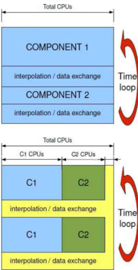
As sketched in Fig. 1, at least two different methods exist to couple the components of an a AO-GCM:
– internal coupling: the different components of the AO-GCM are part of the same executable and share the same parallel decomposition topology. In an operator split-ting approach, the different components (processes) are calculated in sequence. This implies that each task col-lects the required information, and performs the inter-polation between the grids.
– external coupling: the different components (gener-ally an atmosphere GCM and an ocean GCM) of the AO-GCM are executed as separate tasks1, at the same time, i.e. in parallel. An additional external coupler program synchronises the different component models (w.r.t. simulation time) and organises the exchange of data between the different component models. This in-volves the collection of data, the interpolation between different model grids, and the redistribution of data. External coupling is the most widely used method, e.g. by the OASIS coupler (Valcke et al., 2006; Valcke, 2006). The OASIS coupler is used, for example, in the ECHAM5/MPIOM coupled climate model of the Max Planck Institute for Meteorology (Jungclaus et al., 2007) and in the Hadley Centre Global Environment Model (Johns et al., 2006). Also the Community Climate System Model 3 (CCSM3, Collins et al., 2006) adopts a similar technique for information exchange between its different components. Internal coupling is instead largely used in the US, e.g. in the new version of the Community Climate System Model 4 (CCSM4, Gent et al., 2011) and in the Earth System Model-ing Framework (ESMF, Collins et al., 2005).
Following the MESSy standard (J¨ockel et al., 2005), and its modular structure, it is a natural choice to select the in-ternal coupling method as a preferred technique to couple EMAC and MPIOM. In fact, the aim of the MESSy system is to implement the processes of the Earth System as sub-models. Hence, the coupling routines have been developed as part of the MESSy infrastructure as a separate submodel (see A2O submodel below).
3 Coupling MPIOM to EMAC via the MESSy interface
3.1 MPIOM as MESSy submodel
According to the MESSy standard definition, a single time manager clocks all submodels (= processes) in an operator 1task here refers to a process in the distributed memory paralleli-sation model, such as implemented in the Message Passing Interface (MPI)
Fig. 1. Coupling methods between the different model components (C1 and C2) of an AO-GCM (upper panel “internal method”, as im-plemented here, lower panel ”external method” as used for example in the OASIS coupler). The colours denote the different executa-bles.
splitting approach. The MPIOM source code files are com-piled and archived as a library. Minor modifications were re-quired in the source code, and all were enclosed in preproces-sor directives (#ifdef MESSY), which allow to reproduce the legacy code if compiled without this definition. About 20 modifications in 11 different files were required. The major-ity of these modifications are to restrict write statements to one PE (processor), in order to reduce the output to the log-file. The main changes in the original source code modify the input of the initialisation fields (salinity and temperature from the Levitus climatology), with which the ocean model can now be initialised at any date. Another main modifica-tion is related to the selecmodifica-tion of various parameters for cou-pled and non-coucou-pled simulations. In the original MPIOM code, this selection was implemented with preprocessor di-rectives, hence reducing the model flexibility at run-time. In the EMAC-MPIOM coupled system, the preprocessor direc-tives have been substituted by a logical namelist parameter, and in one case (growth.f90) the routines in the coupled case were moved to a new file (growth coupled.f90).
(messy mpiom e5.f90). This file mimics the time loop of MPIOM with the calls to the main entry points to those subroutines, which calculate the ocean dynamics. For the entry points, initialisation, time integration and a finalising phase are distinguished. The MPIOM-library is linked to the model system, operating as a submodel core layer of the MPIOM submodel. Following the MESSy standard, a strict separation of the process formulations from the model infras-tructure (e.g. time management, I/O, parallel decomposition etc.) was implemented. I/O units, for example, are generated dynamically at run-time. In addition, the two model compo-nents (EMAC and MPIOM) use the same high level API (ap-plication programmers interface) to the MPI (Message Pass-ing Interface) library. This implies that the same subroutines (frommo mpi.f90) are used for the data exchange between the tasks in MPIOM and EMAC, respectively.
The new MESSy interface (J¨ockel et al., 2010) introduces the concept of “representations”, which we make use of here. The “representation” is a basic entity of the submodel CHANNEL (J¨ockel et al., 2010), and it allows an easy man-agement of the memory, internal data exchange and output to files. New representations for the ocean variables (2-D and 3-D fields) have been introduced, consistent with the dimen-sioning of the original MPIOM arrays and compatible with the MPIOM parallel domain decomposition. Application of the CHANNEL submodel implies that no more specific out-put routines are required for the ocean model; the outout-put files now have the same format and contain the same meta infor-mation for both the atmosphere and the ocean components. Furthermore, in the CHANNEL API, each “representation” is related to the high-level MPI API via a definition of the gathering (i.e. collecting a field from all tasks) and scatter-ing (i.e. distributscatter-ing a field to all tasks) subroutines. In case of the new MPIOM “representations”, the original gathering and scattering subroutines from MPIOM are applied. As im-plication, the spatial coverage of each core is independently defined for the two AO-GCM components and constrained by the values ofNPXandNPYset in the run-script, both for the atmosphere and for the ocean model. In fact, both mod-els, EMAC and MPIOM, share the same horizontal domain decomposition topology for their grid-point-space represen-tations, in which the global model grid is subdivided into
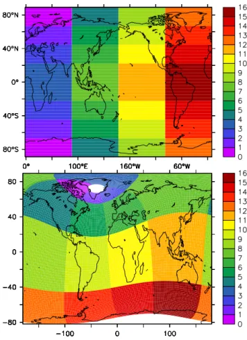
NPXtimesNPYsub-domains (in North-South and East-West direction, respectively, for ECHAM5 and in East-West and North-South direction, respectively for MPIOM). Hence, the same task, which calculates a sub-domain in the atmosphere, also calculates a domain in the ocean, and the two sub-domains do not necessarily match geographically. An exam-ple is shown in Fig. 2, where possible parallel domain de-compositions of EMAC and MPIOM are presented. A total of 16 tasks (specifically withNPX=4 andNPY=4) is used,
and the color indicates the task number in the atmosphere and ocean model, respectively. Other decompositions are possi-ble, depending on the values ofNPXandNPY.
Fig. 2. Parallel (horizontal) “4 times 4” domain decomposition for a model setup with 16 tasks for the atmosphere model (upper panel) and the ocean model (lower panel). The color code denotes the task number.
3.2 The A2O submodel
As described in Sect. 3.1, the two components of the AO-GCM (EMAC and MPIOM) run within the MESSy structure, sharing the same time manager. To couple the two model components (EMAC and MPIOM) physically, some grid-ded information has to be exchanged (see Table 1). For this purpose, a new submodel, named A2O, was developed. In EMAC, a quadratic Gaussian grid (corresponding to the cho-sen triangular spectral truncation) is used, whereas MPIOM operates on a curvilinear rotated grid. The exchanged grid-ded information must therefore be transformed between the different grids.
accumulated fields by the coupling period (in seconds) and resetting the accumulated values to zero. This procedure also allows to change the GCMs time step and/or the coupling fre-quency during run-time.
The submodel A2O (Atmosphere to Ocean, and vice versa) performs the required accumulation/averaging in time and the subsequent grid-transformation. The submodel im-plementation is such that three different setups are possible:
– EMAC and MPIOM are completely decoupled, – EMAC or MPIOM are one-way forced, i.e. one
compo-nent delivers the boundary conditions to the other, but not vice versa,
– EMAC and MPIOM are fully coupled, i.e. the boundary conditions are mutually exchanged in both directions. The setup is controlled by the A2O CPL-namelist, which is described in detail in the Supplement. In Table 1 the vari-ables required for the physical coupling are listed. The fields are interpolated between the grids with a bilinear remap-ping method for scalar fields, while aconservative remap-ping method is used for flux fields (see Sect. 3.3).
For the interpolation the respective weights between the different model grid-points (atmosphere and ocean) are cal-culated during the initialisation phase of the model (see also Sect. 3.3). This allows that any combination of grids and/or parallel decompositions can be used without additional pre-processing.
One of the main advantages of the coupling approach adopted in this study (internal coupling) is the implicit “par-tial” parallelisation of the coupling procedure. Generally, one problem of the coupling routines is that the required in-formation must first be collected from the different tasks of one model component, then processed (e.g. interpolated) and finally re-distributed to the tasks of the other model com-ponent. This process requires a “gathering” of information from different tasks, a subsequent grid transformation, and a “scattering” of the results to the corresponding target tasks. This process is computationally expensive, in particular, if many fields need to be exchanged (as is the case for in-teractive atmosphere-ocean chemistry). In the internal cou-pling approach, only the “gathering” (or collection) and the grid-transformation steps are required. During the initiali-sation phase of the model system, each task (in any of the AO-GCM components) stores the locations (indices) and the corresponding weights required for the transformation from the global domain of the other AO-GCM component. These weights are calculated for the global domain of the other AO-GCM component, because the applied search algorithm (see Sect. 3.3) is sequential and in order to reduce the algorithm complexity in the storage process. Then, within the time in-tegration phase, each task collects the required information from the global field of the other AO-GCM component. Due to this procedure, the interpolation is performed simultane-ously by all tasks (without the need to scatter, i.e. to distribute
information) and thus increasing the coupling performance (see Sect. 4). It must, however, be noted that the new ver-sion of the OASIS coupler (Verver-sion 4; Redler et al., 2010) supports a fully parallel interpolation, which means the in-terpolation is performed in parallel for each intersection of source and target sub-domains. This will potentially increase the run-time performance of OASIS coupled parallel appli-cations.
3.3 Grid-transformation utilising the SCRIP library
For the transformation of fields between the different grids (i.e. from the atmosphere grid to the ocean grid and vice versa), the SCRIP (Spherical Coordinate Remapping and In-terpolation Package) routines (Jones, 1999) are used. These state-of-the-art transformation routines are widely used, for instance in the COSMOS model and the CCSM3 model. The SCRIP routines allow four types of transformations between two different grids:
– first- and second-order conservative remapping (in the MESSy system, only the first order is used),
– bilinear interpolation with local bilinear approximation, – bicubic interpolation,
– inverse-distance-weighted averaging (with a user-specified number of nearest neighbour values).
The library has been embedded into the MESSy2 interface-structure as independent generic module (messy main gridtrafo scrip.f90). For the coupling of EMAC and MPIOM presented here, this module is called by the submodel A2O. It can, however, also be used for grid-transformations by other MESSy submodels. According to the MESSy standard, the parameters used by A2O for the SCRIP library routines can be modified from their default values by changing the A2O submodel CPL-namelist (see the Supplement).
In Fig. 3, an example of a grid transformation with con-servative remapping from the atmosphere grid to the ocean grid is shown. The patterns are preserved and the fluxes are conserved, not only on the global scale but also on the local scale.
4 Analysis of the run-time performance
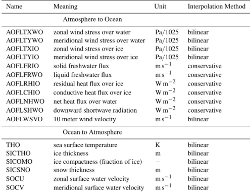
Table 1. Variables to be exchanged by A2O for a physical coupling between EMAC and MPIOM.
Name Meaning Unit Interpolation Method
Atmosphere to Ocean
AOFLTXWO zonal wind stress over water Pa/1025 bilinear AOFLTYWO meridional wind stress over water Pa/1025 bilinear AOFLTXIO zonal wind stress over ice Pa/1025 bilinear AOFLTYIO meridional wind stress over ice Pa/1025 bilinear AOFLFRIO solid freshwater flux m s−1 conservative AOFLFRWO liquid freshwater flux m s−1 conservative AOFLRHIO residual heat flux over ice W m−2 conservative AOFLCHIO conductive heat flux over ice W m−2 conservative AOFLNHWO net heat flux over water W m−2 conservative AOFLSHWO downward shortwave radiation W m−2 conservative AOFLWSVO 10 meter wind velocity m s−1 bilinear
Ocean to Atmosphere
THO sea surface temperature K bilinear
SICTHO ice thickness m bilinear
SICOMO ice compactness (fraction of ice) − bilinear
SICSNO snow thickness m bilinear
SOCU zonal surface water velocity m s−1 bilinear SOCV meridional surface water velocity m s−1 bilinear
MPIOM), differences in the achieved efficiency can be at-tributed to the different coupling methods. In fact, the ef-ficiency of the AO-GCM depends on the efef-ficiency of the component models and on the load balancing between them. For the comparison, we compiled and executed both model systems with the same setup on the same platform: a 64bit Linux cluster, with 24 nodes each equipped with 32 GB RAM and 2 Intel 5440 (2.83 GHz, 4 cores) processors, for a total of 8 cores per node. The Intel Fortran Compiler (ver-sion 11.1.046) together with the MPI-library mvapich2-1.2 has been used with the optimisation option-O1to compile both model codes. The two climate models were run with no output for one month at T31L19 resolution for the sphere and at GR30L40 resolution for the ocean. The atmo-sphere and the ocean model used a 40 and 144 min time-step, respectively. In both cases (EMAC-MPIOM and COSMOS), the same convective and large scale cloud parameterisations were used for the atmosphere, and the same algorithms for advection and diffusion in the ocean, respectively. The ra-diation in the atmosphere was calculated every 2 simulation hours. In addition, the number of tasks requested in the sim-ulation were coincident with the number of cores allocated (i.e. one task per core).
Since in COSMOS the user can distribute a given number of tasks almost arbitrarily between ECHAM5 and MPIOM (one task is always reserved for OASIS), the wall-clock-time required for one simulation with a given number of tasks is not unambiguous. To investigate the distribution of tasks for
the optimum load balance, a number of test simulations are usually required for any given setup. Here, we report only the times achieved with the optimal task distribution. In contrast, EMAC-MPIOM does not require any task distribution opti-misation and the simulation is performed with the maximum possible computational speed.
Three factors contribute to the differences in the model performance:
– The MESSy interface decreases the performance of EMAC in the “GCM-only mode” compared to ECHAM5 by∼3–5 %, and therefore, EMAC-MPIOM is expected to be at least∼ 3–5 % slower than
COS-MOS (see the link “ECHAM5/MESSy Performance” at http://www.messy-interface.org).
– EMAC-MPIOM calculates the interpolation weights during its initialisation phase, whereas COSMOS reads pre-calculated values from files. This calculation is computationally expensive and depends on the AO-GCM component resolutions and on the number of tasks selected. In fact, as seen before in Sect. 3.2, each task calculates the interpolation weights from the global do-main of the other AO-GCM component, with the in-terpolation algorithm scanning the global domain for overlaps with the local domain. This calculation is per-formedonlyduring the initialisation phase.
Fig. 3. Example of a grid transformation with the SCRIP library routines embedded in the generic MESSy submodel MAIN GRIDTRAFO and called by A2O: the precipitation minus evaporation field on the EMAC grid (top) has been transformed to the MPIOM grid (bottom) using the conservative remapping.
number, the single core used by OASIS limits the over-all performance of the COSMOS model.
The total wall-clock-time required to complete the simula-tion of one month shows a constant bias of 58 s for EMAC-MPIOM compared to COSMOS. This bias is independent on the number of tasks used and results from non-parallel pro-cess in EMAC-MPIOM, mainly caused by the different ini-tialisation phases of the two climate models. To analyse the performances of the models, this constant bias has been sub-tracted from the data, so that only the wall-clock times of the model integration phase are investigated. In Fig. 4, the wall-clock times required to complete the integration phase of one month simulation are presented, dependent on the num-ber of cores (= numnum-ber of tasks) used. The wall-clock-times correlate very well between COSMOS and EMAC-MPIOM (see Fig. 4,R2= 0.998), showing that the model scalability
Fig. 4. Scatter plot of the time (seconds wall-clock) required to sim-ulate one month with the COSMOS-1.0.0 model (horizontal axis) and with the EMAC-MPIOM model with the same setup. The color code denotes the number of tasks used (for clarity the number of tasks used are shown also on the top of the points). In these simula-tions one task per core has been used. The regression line is shown in red and the result of the linear regression is denoted in the top left side of the plot. The constant bias of 58 s has been subtracted from the data.
is similar in both cases. Overall, the difference in the perfor-mances can be quantified by the slope of the regression line (see Fig. 4). This slope shows that EMAC-MPIOM has an approx. 10 % better scalability (0.89 times) than COSMOS. In general, the improvement in the performance is due to a re-duction of the gather/scatter operations between the different tasks. In fact, as described in Sect. 3.2, the EMAC-MPIOM model does not perform the transformation as a separate task sequentially, but, instead, performs the interpolation simulta-neously for all tasks in their part of the domain.
It must be stressed that this analysis does not allow a gen-eral conclusion, which is valid for all model setups, res-olutions, task numbers, etc. Most likely, the results ob-tained here are not even to be transferable to other ma-chines/architectures or compilers. However, it is possible to conclude that the coupling method implemented here, does not deteriorate the performance of the coupled model.
5 Evaluation of EMAC-MPIOM
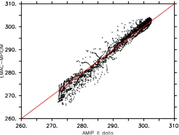
Fig. 5. Scatter plot of 1960–1990 average sea surface temperatures from the Taylor et al. (2000) dataset versus those resulting from simulation TRANS (in K).
model. Therefore, we refer to Jungclaus et al. (2007) for a detailed overview of the model climatology.
The model resolution applied here for the standard simu-lations is T31L19 for the atmosphere component EMAC and GR30L40 for the ocean component MPIOM. This resolution is coarser than the actual state-of-the-art resolution used in climate models. However, near future EMAC-MPIOM sim-ulations with atmospheric and/or ocean chemistry included will be limited by the computational demands and therefore are required to be run at such lower resolutions. It is hence essential to obtain reasonable results at this rather coarse res-olution, which has been yet widely used to couple ECHAM5 with MPIOM. Following the Coupled Model Intercompar-ison Project (CMIP3) recommendations, three simulations have been performed with different Greenhouse gas (GHG) forcings:
– a “preindustrial control simulation” with constant prein-dustrial conditions (GHG of the year 1850), hereafter referred to as PI,
– a “climate of the 20 century” simulation (varying GHG from 1850 to 2000) hereafter referred to as TRANS, and – a “1 % yr−1CO
2increase to doubling” simulation (with other GHG of the year 1850), hereafter referred to as CO2×2.
These simulations have been chosen to allow some of the most important evaluations that can be conducted for climate models of this complexity. In addition, the output from a large variety of well tested and reliable climate models can be used to compare the results with. Because these models had been run at higher resolutions and with slightly different set-ups, some differences in the results are expected, never-theless providing important benchmarks.
Fig. 6. Surface temperature differences between the AMIP II (Tay-lor et al., 2000) dataset and the simulation TRANS (in K). Both datasets have been averaged over the years 1960–1990.
Fig. 7. Global surface temperature anomaly with respect to the 1960–1990 average in K. The lines represent a yearly running mean from simulation TRANS (black) and other IPCC AR4 models (20th century simulations; red: ECHAM5/MPIOM, green: INGV-SXG, blue: UKMO-HadCM3, light blue: IPSL-CM4).
The series of annual values of the GHG for the TRANS simulations have been obtained from the framework of the ENSEMBLES European project and include CO2(Etheridge et al., 1998), CH4 (Etheridge et al., 2002), N2O (Machida et al., 1995) and CFCs (Walker et al., 2000).
5.1 Surface temperature
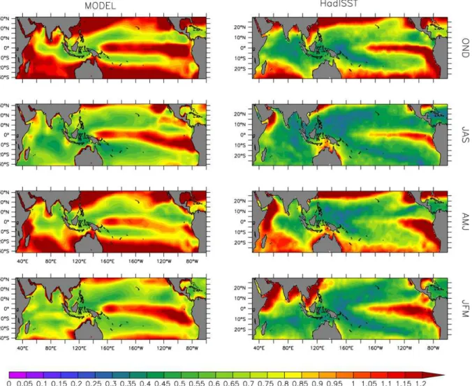
Fig. 8. Standard deviation of the seasonal mean inter-annual variability of the SST (in K). The left and right columns show results from the TRANS simulation, and from the HadISST data (Rayner et al., 2003), respectively, both for the year 1900–1999 (not detrended).
In Fig. 5, the SST of simulation TRANS is compared to the SST from the Atmospheric Model Intercomparison Project (AMIP, Taylor et al., 2000), compiled by Hurrell et al. (2008) based on monthly mean Hadley Centre sea ice and SST data (HadlSST, version 1) and weekly optimum interpolation (OI) SST analysis data (version 2) of the National Oceanic and Atmospheric Administration (NOAA). Both datasets are av-eraged over the years 1960–1990. The correlation between the two datasets is high (R2= 0.97), which confirms that the model is generally correctly reproducing the observed SST.
Although the correlation is high, it is interesting to anal-yse the spatial differences between the AMIPII data and the TRANS simulation. In Fig. 6 the spatial distribution of the differences corresponding to the data shown in Fig. 5 is pre-sented. Although the deviation from the observed values is less than 1 K in most regions over the ocean, in some regions the deviation is larger. The largest biases (up to 6 K) are lo-cated in the North Atlantic and in the Irminger and Labrador Seas in the Northwestern Atlantic. Deviations of similar
Fig. 9. Standard deviation of monthly mean inter-annual variability of the SST (in K) averaged over the NINO3.4 region. The black line shows results from the TRANS simulation, and the red line from the HadISST data (Rayner et al., 2003), both for the year 1900–1999 (not detrended).
The surface temperature changes during the 20th century have been compared with model results provided for the Fourth Assessment Report of the Intergovernmental Panel on Climate Change (IPCC AR4). In Fig. 7, the global av-erage surface temperature increase with respect to the 1960– 1990 average is shown for simulation TRANS in compari-son to a series of simulations by other models, which partic-ipated in the third phase of the World Climate Research Pro-gramme (WCRP) Coupled Model Intercomparison Project (CMIP3, Meehl et al., 2007). The overall increase of the surface temperature is in line with what has been obtained by other climate models of the same complexity. The global surface temperature is somewhat lower compared to those of other models of the CMIP3 database in the 1850–1880 pe-riod, while the trend observed during the 1960–1990 period is very similar for all models.
The tropical ocean seasonal mean inter-annual variability is shown in Fig. 8. It is known that ENSO (El Ni˜no-Southern Oscillation) is the dominating signal of the variability in the Tropical Pacific Ocean region. Although in the East Pacific the simulated variability correlates well with the observed one (see Fig. 8), in the western Tropical Pacific, the model generates a somewhat higher inter-annual variability, which is absent in the observations. The cause is most probably the low resolution of the models. The ocean model, as applied here, has a curvilinear rotated grid with the lowest resolution in the Pacific Ocean (see also AchutaRao and Sperber (2006, and references therein) for a review on ENSO simulations in climate models). Although the variability is generally higher in the model than in the observations, an ENSO signal is observed, as shown in Fig. 9. In this figure, the monthly variability of the SST is depicted for the so called ENSO re-gion 3.4 (i.e. between 170◦ and 120◦W and between 5◦S
and 5◦N). The model variability is confirmed to be higher than the observed one; nevertheless, the model reproduces the correct seasonal phase of El Ni˜no, with a peak of the SST anomaly in the boreal winter. Compared to the diffi-culties in representing the correct inter-annual variability in the Pacific Ocean, in the Indian Ocean the model reproduces the observed patterns with better agreement to the observa-tions. During July, August and September the model repro-duces (with a slight overestimation) the correct variability in the central Indian Ocean, while the patterns produced by the model are qualitatively similar to the observed one dur-ing April, May and June. The model is, however, strongly overestimating the variability during October, November and December in the Indian Ocean, especially in the Southern part, while in January, February and March the simulated open ocean shows a too high inter-annual variability over the central-south Indian Ocean and a too low variability near the Northern coasts.
5.2 Ice coverage
Observations Simulation Observations Simulation
March
September
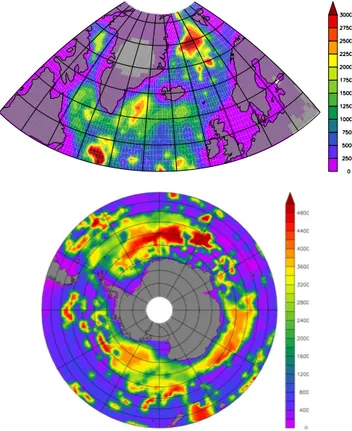
Fig. 10.Simulated and observed polar ice coverage. The upper and lower rows show March and September, respectively. Observations and results from simulation TRANS are averaged for the years 1960–1990. Observations are from the HadISST (Rayner et al., 2003) data set.
Fig. 11. Global sea ice coverage (in 1012m2). The black line shows the HadISST (Rayner et al., 2003) data, while the blue and the red lines represent the model results from simulations PI and TRANS, respectively. Dashed and solid lines represent annual and decadal running means, respectively.
To compare the changes of the sea ice coverage during the 20th century, the annual sea ice coverage area has been cal-culated from the simulations TRANS and PI and compared with the dataset by Rayner et al. (2003), which is based on observations (see Fig. 11). The simulated sea ice coverage agrees with the observations, although with an overestima-tion (up to≃8 %). In addition, the simulated inter-annual
variability is much larger than what is observed. Neverthe-less the model is able to mimic the decrease in the sea ice area coverage observed after 1950, although with a general overestimation.
5.3 Thermohaline circulation and meridional overturning circulation
Fig. 12. Maximum depth (m) of vertical convection for the years 1900–1999 of simulation TRANS.
and appears to be well simulated by the model. In the SH, convection occurs mainly outside the Weddel Sea and Ross Sea, with some small convective events all around the South-ern Ocean and with the major events occurring between 0 and 45◦E.
5.4 Jet streams
The jet streams are strong air currents concentrated within a narrow region in the upper troposphere. The predominant one, the polar-front jet, is associated with synoptic weather systems at mid-latitudes.
Hereafter, jet stream always refers to the polar-front jet. The adequate representation of the jet stream by a model indicates that the horizontal temperature gradient (the main cause of these thermal winds) is reproduced correctly. In Fig. 13, the results from simulation TRANS are compared with the NCEP/NCAR (National Centers for Environmental Prediction/ National Center for Atmospheric Research) Re-analysis (Kalnay et al., 1996). The maximum zonal wind speed is reproduced well by the model, with the SH jet stream somewhat stronger than the NH jet stream (≃30 and ≃22 m s−1, respectively). The location of the maximum
wind, however, is slightly shifted poleward by≃5◦. The
ver-tical position of the jet streams is also≃50 hPa higher than
the observed. The NH jet stream has a meridional extension
Fig. 13. Climatologically averaged zonal wind. The color denotes the wind speed in m s−1as calculated from simulation TRANS for the years 1968–1996, while the contour lines denote the wind speed calculated from the NCEP/NCAR Reanalysis 1 for the same years. The vertical axis is in hPa.
which is in line with what is observed, while the simulated SH jet stream is narrower in the latitudinal direction com-pared to the re-analysis provided by NCEP. In fact, the av-eraged zonal wind speed higher than 26 m s−1in the SH is located between≃40–30◦S in the model results, while it is
distributed on a larger latitudinal range (≃50–25◦S) in the
NCEP re-analysis data. Finally, while the NCEP data show a change of direction between the tropical and extratropical zonal winds, the simulation TRANS reproduces such fea-tures only in the lower troposphere and in the stratosphere, while in the upper troposphere (at around 200 hPa) westerly winds still dominate. Although some differences arise from the comparison, the general features of thermal winds are re-produced correctly by the model, despite the low resolution used for the atmosphere model (T31L19).
5.5 Precipitation
Fig. 14. Zonally averaged difference in the precipitation rate (in mm day−1) between climatologies derived from simulation TRANS (1950–2000) and from observations (Global Precipitation Climatology Project, 1979–2009, Adler et al., 2003).
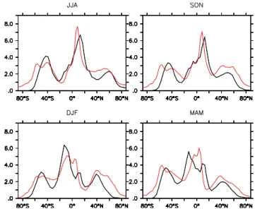
a distinct minimum at around 30◦S, which is weaker in the observations. Finally, the model largely underestimates the precipitation over Antarctica throughout the year and in the storm track during the NH winter. This is associated with the underestimation of the sea surface temperature in these regions.
5.6 Climate sensitivity
To estimate the climate sensitivity of the coupled model EMAC-MPIOM, the results from the CO2×2 simulation are
analysed. The simulation yields a global average increase of the surface temperature of 2.8 K for a doubling of CO2. As mentioned in the IPCC AR4, the increase in the temperature for a CO2doubling “is likely to be in the range 2 to 4.5◦C with a best estimate of about 3◦C”. The value obtained in this study is thus in line with results from the CMIP3 multi-model dataset. For the same experiment, for example, the mod-els ECHAM5/MPIOM (with OASIS coupler) and INGV-SX6 show an increase of the global mean surface tempera-ture of 3.35 K and 1.86 K, respectively. To calculate the cli-mate sensitivity of the model, the mean radiative forcing at the tropopause (simulation CO2×2) was calculated for the
years 1960–1990 as 4.0 W m−2. This implies a climate sen-sitivity of the model of 0.7 K W−1m2, in line with what has been estimated by most models from the CMIP3 dataset (e.g. ECHAM5/MPIOM, INGV-SX6, INM-CM3 and IPSL-CM4 with 0.83, 0.78, 0.52 and 1.26 K W−1m2, respectively). De-spite the usage of the same dynamical components, EMAC-MPIOM and ECHAM5/EMAC-MPIOM do not present the same climate sensitivity, because of the different resolution and boundary conditions (GHG vertical profiles) used in the model simulations here considered.
Fig. 15. Seasonal zonal average of climatological precipitation rate (in mm day−1). The red lines show observations from the Global Precipitation Climatology Project (1979–2009 climatology), the black lines represent results from the simulation TRANS (1950– 2000 climatology).
6 Summary and outlook
A new internal coupling method, based on the MESSy inter-face, between EMAC and MPIOM is presented. It shows a comparable run-time performance as the external COSMOS coupling approach using OASIS3 under comparable condi-tions and for the set-up tested here. Despite the fact that the effective performances of the model components are not de-teriorated by the new approach, it is hardly possible to esti-mate in general which coupling method yields the best per-formance of the climate model, because it is determined by the number of available tasks, the achievable load balance, the model resolution and complexity, and the single compo-nent scalability. Additionally, the scaling and load imbal-ance issues cannot be regarded separately, rendering a gen-eral statement about the performance and scaling features of the internal versus external coupling method hardly possible. The efforts for implementing either the internal or the exter-nal coupling approach primarily depend on the code struc-ture of the legacy models to be coupled. In both cases, the legacy codes need to be equipped with additional infrastruc-ture defining the interfaces. The external approach is by de-sign potentially more favourable for less structured codes. Hence, in most cases, the external approach requires smaller coding effort to be implemented than the internal approach.
Following the MESSy philosophy, a new submodel (named A2O) was developed to control the exchange of information (coupling) between the AO-GCM components. However, since this submodel is flexibly controlled by a namelist, it can be used to convert any field present in one AO-GCM component to the other one and vice versa. Thanks to this capability, A2O can be used not only to control the physical coupling between the two AO-GCM components, but also to exchange additional information/fields between the two domains of the AO-GCM, including physical and chemical (e.g. tracer mixing ratios) data. Hence, as a future model development, the ocean biogeochemistry will be in-cluded via the MESSy interface and coupled to the air chem-istry submodels of EMAC, using the AIRSEA submodel pre-viously developed (Pozzer et al., 2006). This will allow a complete interaction between the two AO-GCM domains, exchanging not only quantities necessary for the physical coupling of EMAC and MPIOM (i.e. heat, mass and mo-mentum as shown here) but also chemical species of atmo-spheric or oceanic interest, leading to a significant advance-ment towards a more detailed description of biogeochemical processes in the Earth system.
Supplementary material related to this article is available online at:
http://www.geosci-model-dev.net/4/771/2011/ gmd-4-771-2011-supplement.pdf.
Acknowledgements. The authors wish to thank the referees and especially S. Valcke, who helped improve the quality of the manuscript. B. Kern acknowledges the financial support by the In-ternational Max Planck Research School for Atmospheric Chem-istry and Physics. The authors wish to thank J. Lelieveld for the contribution and support in the preparation of this manuscript. We thank also the DEISA Consortium (www.deisa.eu), co-funded through the EU FP6 project 031513 and the FP7 project RI-222919, for support within the DEISA Extreme Computing Ini-tiative. The simulations for this study have been performed in the DEISA grid (project “ChESS”). We acknowledge the modeling groups, the Program for Climate Model Diagnosis and Intercom-parison (PCMDI) and the World Climate Research Programme’s (WCRP) Working Group on Coupled Modelling (WAO-GCM) for their roles in making available the WCRP Coupled Model Inter-comparison Project phase 3 multi-model dataset. Support of this dataset is provided by the Office of Science, US Department of Energy. We acknowledge also the NOAA/OAR/ESRL PSD, Boul-der, Colorado, USA, for providing the NCEP Reanalysis data, on their web site at http://www.esrl.noaa.gov/psd/. We acknowledge the usage of data from the ENSEMBLE project (contract number GOCE-CT-2003-505539).We acknowledge support from the Euro-pean Research Council (ERC) under the C8 project. We acknowl-edge the ENIGMA (http://enigma.zmaw.de) network for support. We finally acknowledge the use of the Ferret program for analy-sis and graphics in this paper. Ferret is a product of NOAA’s Pa-cific Marine Environmental Laboratory (information is available at http://www.ferret.noaa.gov).
The service charges for this open access publication have been covered by the Max Planck Society.
Edited by: W. Hazeleger
References
AchutaRao, K. and Sperber, J.: ENSO simulation in coupled ocean-atmosphere models: are the current models better?, Clim. Dy-nam., 27, 1–15, doi:10.1007/s00382-006-0119-7, 2006. Adler, R., Huffman, G., Chang, A., Ferraro, R., Xie, P., Janowiaks,
J., Rudolf, B., Schneider, U., Curtis, S., Bolvin, D., Gruber, A., and Susskind, P. A.: The Version 2 Global Precipitation Cli-matology Project (GPCP) Monthly Precipitation Analysis (1979-Present), J. Hydrometeorol., 4, 1147–1167, 2003.
Arzel, O., Fichefet, T., and Goosse, H.: Sea ice evolution over the 20th and 21st centuries as simulated by current AOGCMs, Ocean Model., 12, 401–415, doi:10.1016/j.ocemod.2005.08.002, 2006. Collins, N., Theurich, G., Deluca, C., Suarez, M., Trayanov, A., Balaji, V., Li, P., Yang, W., Hill, C., and Da Silva, A.: De-sign and implementation of components in the earth system modeling framework, Int. J. High Perform. C., 19, 341–350, doi:10.1177/1094342005056120, 2005.
Collins, W., Bitz, C. M., Blackmon, M. L., Bonan, G. B., Brether-ton, C. S., CarBrether-ton, J. A., Chang, P., Doney, S. C., Hack, J. J., Henderson, T. B., Kiehl, J. T., Large, W. G., McKenna, D. S., Santer, B. D., and Smith, R. D.: The Community Climate Sys-tem Model Version 3 (CCSM3), J. Climate, 19(11), 2122–2143, 2006.
Dai, A.: Precipitation Characteristics in Eighteen Coupled Climate Models, J. Climate, 19, 4605–4630, doi:10.1175/JCLI3884.1, http://journals.ametsoc.org/doi/abs/10.1175/JCLI3884.1, 2006. Etheridge, D., Steele, L. P., Langenfelds, R., Francey, R. J., Barnola,
J.-M., and Morgan, V.: Historical CO2 Records from the Law Dome DE08, DE08-2, and DSS Ice Cores, Trends: A Com-pendium of Data on Global Change. Carbon Dioxide Informa-tion Analysis Cente, Oak Ridge NaInforma-tional Laboratory, US Depart-ment of Energy, Oak Ridge, Tenn., USA, http://cdiac.esd.ornl. gov/trends/co2/lawdome.html, 1998.
Etheridge, D., Steele, L. P., Francey, R., and Langenfelds, R.: His-torical CH4 Records Since About 1000 A.D., From Ice Core Data, Trends: A Compendium of Data on Global Change. Carbon Dioxide Information Analysis Center, Oak Ridge Na-tional Laboratory, US Department of Energy, Oak Ridge, Tenn., USA, http://cdiac.ornl.gov/trends/atm meth/lawdome meth.html, 2002.
Gent, P. R., Danabasoglu, G., Donner, L. J., Holland, M., Hunke, E., Jayne, S. R., Lawrence, D., Neale, R., Rasch, P., Vertenstein, M., Worley, P., Yang, Z.-L., and Zhang, M.: The Community Climate System Model version 4, J. Climate, doi:10.1175/2011JCLI4083.1, in press, 2011.
Houghton, J. T., Ding, Y., Griggs, D. J., Nouger, M., van der Lin-den, P. J., Dai, X., Maskell, K., and Johnson, C. A.: IPCC – Cli-mate Change 2001: The Scientific Basis. Contribution of Work-ing Group I to the third Assessment Report of the Intergovern-mental Panel on Climate Change, Cambridge University Press, 2001.
Commu-nity Atmosphere Model, J. Climate, 21, 5145–5153, 2008. J¨ockel, P., Sander, R., Kerkweg, A., Tost, H., and Lelieveld, J.:
Technical Note: The Modular Earth Submodel System (MESSy) – a new approach towards Earth System Modeling, Atmos. Chem. Phys., 5, 433–444, doi:10.5194/acp-5-433-2005, 2005. J¨ockel, P., Tost, H., Pozzer, A., Br¨uhl, C., Buchholz, J., Ganzeveld,
L., Hoor, P., Kerkweg, A., Lawrence, M. G., Sander, R., Steil, B., Stiller, G., Tanarhte, M., Taraborrelli, D., van Aardenne, J., and Lelieveld, J.: The atmospheric chemistry general circulation model ECHAM5/MESSy1: consistent simulation of ozone from the surface to the mesosphere, Atmos. Chem. Phys., 6, 5067– 5104, doi:10.5194/acp-6-5067-2006, 2006.
J¨ockel, P., Kerkweg, A., Pozzer, A., Sander, R., Tost, H., Riede, H., Baumgaertner, A., Gromov, S., and Kern, B.: Development cycle 2 of the Modular Earth Submodel System (MESSy2), Geosci. Model Dev., 3, 717–752, doi:10.5194/gmd-3-717-2010, 2010. Johns, T. C., Durman, C. F., Banks, H. T., Roberts, M. J., McLaren,
A. J., Ridley, J. K., Senior, C. A., Williams, K. D., Jones, A., Rickard, G. J., Cusack, S., Ingram, W. J., Crucifix, M., Sexton, D. M. H., Joshi, M. M., Dong, B.-W., Spencer, H., Hill, R. S. R., Gregory, J. M., Keen, A. B., Pardaens, A. K., Lowe, J. A., Bodas-Salcedo, A., Stark, S., and Searl, Y.: The new Hadley Centre climate model (HadGEM1): Evaluation of coupled simulations, J. Climate, 19, 1327–1353, doi:10.1175/JCLI3712.1, 2006. Jones, P.: First- and Second-Order Conservative Remapping
Schemes for Grids in Spherical Coordinates, Mon. Weather Rev., 127, 2204–2210, 1999.
Jungclaus, J. H., N.Keenlyside, Botzet, M., Haak, H., Luo, J.-J., Latif, M., Marotzke, J., Mikolajewicz, U., and Roeckner, E.: Ocean Circulation and Tropical Variability in the Coupled Model ECHAM5/MPI-OM, J. Clim., 19, 3952–3972, 2007.
Kalnay, E., Kanamitsu, M., Kistler, R., Collins, W., Deaven, D., Gandin, L., Iredell, M., Saha, S., White, G., Woollen, J., Zhu, Y., Leetmaa, A., Reynolds, R., Chelliah, M., Ebisuzaki, W., Higgins, W., Janowiak, J., Mo, K. C., Ropelewski, C., Wang, J., Jenne, R., and Josep, D.: The NCEP/NCAR 40-year reanalysis project, B. Am. Meteorol. Soc., 77, 437–471, 1996.
Machida, T., Nakazawa, T., Fujii, Y., Aoki, S., and Watanabe, O.: Increase in the atmospheric nitrous oxide concentration dur-ing the last 250 years, Geophys. Res. Lett., 22, 2921–2924, doi:10.1029/95GL02822, 1995.
Marsland, S., Haak, H., Jungclaus, J. H., Latif, M., and R¨oske, F.: The Max- Planck-Institute global ocean/sea ice model with orthogonal curvilinear coordinates, Ocean Model., 5, 91–127, 2003.
Meehl, G. A., Covey, C., Delworth, T., Latif, M., Mcavaney, B., Mitchell, J. F. B., Stouffer, R. J., and Taylor, K. E.: THE WCRP CMIP3 Multimodel Dataset: A New Era in Climate Change Research, B. Am. Meteorol. Soc., 88, 1383–1394, doi:10.1175/BAMS-88-9-1383, 2007.
Pickart, R. S., Torres, D. J., and Clarke, R. A.: Hy-drography of the Labrador Sea during Active Convec-tion, J. Phys. Ocean., 32, 428–457, doi:10.1175/1520-0485(2002)032¡0428:HOTLSD¿2.0.CO;2, 2002.
Pozzer, A., J¨ockel, P., Sander, R., Williams, J., Ganzeveld, L., and Lelieveld, J.: Technical Note: The MESSy-submodel AIRSEA calculating the air-sea exchange of chemical species, Atmos. Chem. Phys., 6, 5435–5444, doi:10.5194/acp-6-5435-2006, 2006.
Rayner, N. A., Parker, D., Horton, E., Folland, C., Alexan-der, L., Rowell, D., Kent, E., and Kaplan, A.: Global anal-ysis of SST, sea ice and night marine air temperature since the late nineteenth century, J. Geophys. Res., 108, 4407, doi:10.1029/2002JD002670, 2003.
Redler, R., Valcke, S., and Ritzdorf, H.: OASIS4 – a coupling soft-ware for next generation earth system modelling, Geosci. Model Dev., 3, 87–104, doi:10.5194/gmd-3-87-2010, 2010.
Roberts, M. J., Banks, H., Gedney, N., Gregory, J., Hill, R., Mullerworth, S., Pardaens, A., Rickard, G., Thorpe, R., and Wood, R.: Impact of an Eddy-Permitting Ocean Res-olution on Control and Climate Change Simulations with a Global Coupled GCM, J. Climate, 17, 3–20, doi:10.1175/1520-0442(2004)017¡0003:IOAEOR¿2.0.CO;2, 2004.
Roeckner, E., Brokopf, R., Esch, M., Giorgetta, M., Hagemann, S., Kornblueh, L., Manzini, E., Schlese, U., and Schulzweida, U.: Sensitivity of simulated climate to horizontal and vertical resolution in the ECHAM5 atmosphere model, J. Climate, 19, 3771–3791, 2006.
Sausen, R. and Voss, R.: Part I: Techniques for asyn-chronous and periodically synasyn-chronous coupling of atmosphere and ocean models, Clim. Dynam., Springer, 12, 313–323, doi:10.1007/BF00231105, 1996.
Taylor, K., Williamson, D., and Zwiers, F.: The sea surface temper-ature and sea ice concentration boundary conditions for AMIP II simulations; PCMDI Report, Tech. Rep. 60, Program for Climate Model Diagnosis and Intercomparison, 2000.
Valcke, S.: OASIS3 User Guide, Technical report no. 3, CERFACS, PRISM Support Initiative, 2006.
Valcke, S., Guilyardi, E., and Larsson, C.: PRISM and ENES: A European approach to Earth system modelling, Concurrency Computat., Pract. Exper., 18(2), 231–245, 2006.
Walker, S. J., Weiss, R., and Salameh, P.: Reconstructed histories of the annual mean atmospheric mole fractions for the halocar-bons CFC-11 CFC-12, CFC-113, and carbon tetrachloride, J. Geophys. Res., 105, 14285–14296, doi:10.1029/1999JC900273, 2000.