C
OND
C
LOSE
: new algorithm of association rules extraction
Hamida AMDOUNI1, Mohamed Mohsen GAMMOUDI21Computer Science Department, FST Tunisia
Member of Research Laboratory RIADI
2Higher School of Statistics and Information Analysis University of Carthage,
Member of Research Laboratory RIADI Charguia II, Tunisia
Abstract
Several Methods are proposed for associate rule generation. They try to solve two problems related to redundancy and relevance of associate rules. In this paper we introduce a method called CONDCLOSE which provides the reduction of PRINCE algorithm run-time proposed by Hamrouni and al. in 2005.In fact, we show how the notions of pseudo context and condensed context which we introduce in this paper allows us to attempt these three objectives: no redundancy, relevance of associate rules and minimizing run time of associate rule extraction.
Keywords: Associate rule, Minimal generator extraction, Pseudo context, condensed context.
1. Introduction
The extraction of association rules from transactional database was the object of several research departing from those of Agrawal [1]. However, the problems of the redundancy and the quality of the extracted rules still exist [2, 5, 6, 14, 16].
Indeed, we are interested in the last researches to this problem.
As far as we are concerned, an approach introduced by [12] consists on extracting a subset of non-redundant rules and without losing any information [3]. This latter is based on the mathematical foundations of the Formal Analysis of Concepts (FCA) [7]. Its principle is to extract a sub-set of Itemsets called Closed Itemsets from which a subset of rules is generated.
In spite of these efforts, the volume of rules remains important. For this reason, the researches of [15] were realized to introduce the notion of minimal generators. Indeed, the minimal generators are a minimal set of items the closure of which allows to generate all the closed Itemsets [13, 15, 17].
However [9] noticed that the relation of partial order between the minimal generators allows to reduce the volume of association rules and he presents an algorithm
called PRINCE. But, as it was mentioned in [9, 11], the
runtime of minimal generators extraction as well as that their organization in partial order remains exponential. In this article, we present a n ew method called CONDCLOSE to reduce the run time by acting on the three steps defined in [9].
Before explaining in details our contribution, we are going to introduce in the first section, some basic concepts necessary to facilitate the understanding of our method. In the second section, we will present the principle of the PRINCE algorithm. In the third section, we are going to
illustrate our method with an example. Afterward, we will make a comparative study with the PRINCE algorithm in
order to present our contribution.
2. Basic notions
• Formal context: let (O, I, R) be a triplet with O and I are respectively sets of objects (eg. transactions), sets of items and R ⊆ O x I is a b inary relation between objects and items.
• Itemset: It is a nonempty subset of items. An itemset consisting of k elements is called k-itemset.
• Support of an i temset: the frequency of simultaneous occurrence of an itemset (I’) in the set of objects called Supp(I’).
• Frequent itemset (FI): FI is a set of items whose support ≥ a user-specified threshold called minsup. All its subsets are frequent. The set of all frequent itemsets called SFI.
• Associative rule: Any association rule having the following form: A B, where A and B are disjoint itemsets with A is its premise (condition) and B is its conclusion.
• Confidence: The confidence of an association rule A
B measures how often items in B appear in objects that contain A:
Supp(A,B): the number of objects that the itemset A and the itemset B share.
o Supp(A): le number of objects that contain A. Based on the degree of confidence, association rules can be classified as follows:
o Exact rule: rule which confidence = 1
o Approximative rule: rule which confidence < 1 o Valid rule: rule which confidence ≥ a
user-specified threshold called minconf
• Galois connection: In A formal context K is a triplet K = (O, I, R), For every set of objects A ⊆ O, the set f(A) of attributes in relation R with the objects of A is as follow:
(2)
Dually, for every set of attributes B ⊆ I, the set g(B) of objects in relation R with the attributes of B is as follow:
(3) The two functions f and g defined between objects and attributes form a Galois connection.
The operators f ° g(B) and g ° f(A) called φ are the closure operators.
φ verifies the following properties ∀X, Y ⊆ I (resp. ∀X1, Y1⊆ O):
(4) (5) (6) • Frequent Closed Itemset (FCI): An Itemset I’ is called
closed if I’ = φ(I’). In other words, an itemset I’ is closed if the intersect of the objects to which I’ belongs is equal to I’ and it is frequent if its support ≥ minsup. SFCI is the Set of Frequent Closed Itemset.
• Minimal Generator: An Itemset c ⊆ I is a cl osed Itemset generator I’ ⇔ φ(c) = I ’. c i s a m inimal frequent generator if its support is ≥ minsup.
The set of frequent minimal generators of I’ called GMFI’’
(7)
• Negative border (GBd-): the set on no-frequents minimal generator.
• Positive border (GBd+): Let GMFk is the set of all minimal frequent generators:
(8)
• Equivalent classes: The closure operator φ divides the set of frequents Itemsets into disjoint equivalent classes including elements having the same support. The largest element in a given class is an FCI called I’ and smaller ones are the GMFI’ [12].
• Comparable equivalent classes: The classes Ci and Cj are only said comparable if FCI of Ci covers that of Cj. The five following notions are defined in [7]:
• Formal concept: a formal concept is a m aximal objects-attributes subset where objects and attributes are in relation. More formally, it is a pair (A, B) with A ⊆ O and B ⊆ I, which verifies f(A) = B and g(B) = A. A is the extent of the concept and B is its intent.
• Partial order relation between concepts≤: The partial order relation called ≤ is defined as follow: for two formal concepts (A1, B1) and (A2, B2): (A1, B1) ≤ (A2, B2) ⇔ A2⊆ A1 and B1⊆B2.
• Meet / Join: for each concepts (A1, B1) and (A2, B2), it exist a greatest lower bound (resp. a least upper bound) called Meet (resp. Join) denoted as ((A1, B1) ∧ (A2, B2) (resp. (A1, B1) ∨ (A2, B2)) defined by:
(9)
(10)
• Galois lattice: The Galois lattice associated to a formal context K is a graph composed of a set of formal concepts equipped with the partial order relation ≤. This graph is a representation of all the possible maximal correspondences between a subset of objects O and a subset of attributes I.
• Frequent minimal generators lattice: A partial ordered structure of which each equivalent class includes the appropriate frequent minimal generators [4].
• Iceberg lattice: A partial ordered structure of frequent closed Itemsets having only the join operator. It is considered a superior semi-lattice [15].
• Generic base of exact associative rules and Informative base of approximative associative rules: Generic base of exact associative rules (GBE) is a base composed of non-redundant generic rules having a confidence ratio equal to 1 [3]. Given a context (O, I, R), the set of frequent closed itemsets (SFCI) and the set of minimal generators GMFk :
(11) While informative base of approximative associative
(GBA) rules is defined as follows:
(12)
The union of those bases constitutes a g eneric base without losing information.
3. Principle of P
RINCEalgorithm
equal to the cardinality of the initial context). It determines, all k-generator candidates and by doing this, at each level k, a self-join of (k-1)-generators. Subsequently, it eliminates any candidate of size k if at least one of its subsets is not a minimal generator or if its support is equal to one of them. GMFk is the union of all sets of frequent minimal generators determined in each level, while no-frequents form the GBd-.
Second, GMFk and GBd- be used to form a minimal generators lattice and this by comparing each minimal generator g to the list L of immediate successors of its subsets of size k-1. If L is empty then g is added to this list, otherwise, four cases are possible for each g1∈ L knowing that Cg and Cg1 are the equivalence classes of g and g1: • If (g∪g1) is a minimal generator then Cg and Cg1 are
no-comparables.
• If Supp(g) = Supp(g1) = Supp(g∪g1) then g and g1∈ a same class.
• If Supp(g) < Supp(g1) = Supp(g∪g1) then g become the successor of g1.
• If Supp(g) < Supp(g1) ≠ Supp(g∪g1) then Cg and Cg1 are no-comparables.
If (g∪g1) is not a minimal generator, the calculation of its support is performed by applying this proposal [15]: Let GMk = GMFk ∪ GBd- (set of all generators), an itemset I’ is no-generator if:
(13)
The research process of Supp(g∪g1) stops whene one of its subsets has a strictly lower support than that of g and g1 because this implies that Cg and Cg1are no-comparables. After constructing the minimal generators lattice, PRINCE
determines for each equivalence class, starting from C∅ to
the top, the frequent closed itemset and built the Iceberg lattice by applying this proposal:
Let I1 and I2 are two frequent closed itemsets such as I1 covers I2 by the partial order relation and GMFI1 is the set of the frequent minimal generator of I1:
(14) The two lattices are used to extract exact and approximative rules. Note that the rules with confidence = 1 are exact and an implications extracted from each node (intra-node). Whereas, the approximative rules have confidence ≥ minconf are implications involving two comparable equivalence classes. These rules are implications between nodes.
As proved in [9] all generated rules are no redundant and guarantee that there is no loss of information. But it should be noted that the complexity of the first step (the extraction of frequent minimal generators) is exponential, which implies an overall processing time high in the case of scattered contexts.
4. Proposed Method
Before presenting our method, we are going to define two notions:
• Pseudo context: is a triplet (O’, I’, R’) with O’ and I’ are respectively sets of objects, sets of Itemsets and R’ ⊆ O’ x I’ is a b inary relation between objects and Itemsets.
• Condensed Context: is a t riplet (O”, I”, R”) created from pseudo context (O’, I’, R’); with O” is a set of objects ∈ O’, I” is formed of sets of Itemsets ∈ I’ called {I} and R’’ ⊆ O” x I” is a b inary relation between O” and I”. Any couple (o, {I}) ∈ R” indicate the fact that the object o ∈ O” is associated to the Itemsets of {I} which ∈ I”.
In fact, to extract non redundant rules and without losing information by minimizing the time of the treatment, we present a n ew algorithm called CONDCLOSE (Closed
Condensed) based on the notion of condensed context. It contains three steps. The first one allows to extract the frequent minimal generators as well as the positive border (GBd +) by condensing the initial context.
The second one uses the minimal generators and the condensed context results to construct a frequent minimal generators lattice. The last step determines the generic base of exact and approximative rules associated to the lattice.
The algorithm CONDCLOSE is presented as follows:
Algorithm CONDCLOSE
Input : C extraction context ; s minsup ; f minconf Ouput : GBE ; GBA
Begin
EXT-GEN-COND(C, GMF, GBd+, C”)
// Extraction of minimal generators and GBd+
CONS-GEN-LATTICE(GMF, GBd+, C”, Tgen) // Construction of minimal generators lattice DETERM-GBE-GBA(Tgen,GBE, GBA)
// Determine GBE, GBA
return(GBE, GBA) End
4.1 Extraction of minimal generators
In this section, we present the algorithm EXT-GEN-COND
which allows to extract the frequent minimal generators (GMFk) and the positive border (GBd+) by using the notion of condensed context.
In fact, we use the initial context to extract the 1-frequent generators. Afterward, we make a self-join of this set in order to determine the 2-candidate generators. Every candidate having minimal generators subsets, a s upport different to the support of its subsets and upper to the minsup will be added to the list of the frequent minimal generators. The candidate having an equal support at least to the support of one of their subsets is going to be stored in a positive border (GBd+).
Having determined the 2-frequent generators, we concatenate the columns of their subsets. This new context is called pseudo context and it is used during the research of the 3-minimal generators.
Then, a new pseudo context will be created with the same principle which is a co ncatenation of the columns of the subsets of the 3-generators.
Finally, the process stops when there are no generators to be determined.
The last pseudo context is used to form a new condensed context by grouping the Itemsets which share the same objects in a single column. This condensed context as well as the list of the minimal generators and the positive border will be used in the second step.
The algorithm EXT-GEN-COND is presented as follows,
knowing that:
• GMF: set of frequent minimal generators. • GBd+: positive border
• Gk: set of generators size k
• ELIMINATE: Having the set of generators, this function
eliminate the generators that the support < minsup. • DETERM-GENERATOR: it is the function which takes in
input Gk and return the set of (k+1)- generators. This is done by making a self-joint of k-generators and
by eliminating every candidate of size (k+1) non generator. A candidate is called non generator if at least one of its subsets is not. Or its support is equal to that of the one of them. The calculation of the support of the subsets is made by using the condensed context. This function also allows to save the candidate
generators which have the same support as one of their subsets in GBd+.
• CONS-PSEUDO-CONT: allows to create a pseudo context
by grouping the columns of the subsets of every element of the list of k-generators in input.
• CONS-COND-CONCEPTS: it is the function which allows
to group the columns of Itemsets which share the same objects.
Algorithm EXT-GEN-COND
Input : C extraction contexte ; s minsup
Output : GMF ; GBd+ ; C’’ condensed contexte
Begin
C’ ← C ; GMF ←∅ ; GBd+ ←∅ ; k ← 1 G1 ← list of 1-itemsets
G1← ELIMINATE (G1,s) while Gk.gen ≠ ∅ do
Gk+1 ← DETERM-GENERATOR(Gk, C’, GBd+) C’← CONS-PSEUDO-CONT(Gk+1, C’) GMF ← GMF ∪ Gk
k ← k + 1 end while
C’’← CONS-COND-CONCEPTS(C’)
return(GMF ; GBd+ ; C’’) End
Example 1:
We present an illustrative example to explain the detailed progress of the first step.
Let’s be the binary context (O, I, R) as follows, minsup = 2 and minconf = 0,5:
R a1 a2 a3 a4 a5
o1 1 0 1 1 0
o2 0 1 1 0 1
o3 1 1 1 0 1
o4 0 1 0 0 1
o5 1 1 1 0 1
Fig. 1: Initial context
• The list of 1-frequent generators put in an increasing order of support = {a1:3, a2:4, a3:4, a5: 4}; GBd+ = ∅.
• The determination of 2-frequent generators consists in making a self-joint of the elements of the 1-generators set and in eliminating every 2-candidate generator if at least one of its subsets has no minimal generator or if its support is equal to that of the one of them.
We start with joining {a1} and {a2}, the 2-candidate generator = {a 1a2}, its support = 2 = minsup ≠ Supp({a1}) ≠ Supp({a2}) so the first 2 -frequent generator = {a1a2 : 2}.
Afterwards, by joining {a1} and {a3}, the 2-candidate generator = {a1a3}, its support = 3 > minsup but = Supp({a1}). So, it is not added to the list of 2-frequent generators and it will be added to GBd+ which becomes = {a1a3 : 3}.
O
:
se
t o
f o
bje
cts
In the case of the joint of {a1} and {a5}, the support of 2-candidate generator {a1a5} = 2 = m insup ≠ Supp({a1}) and Supp({a5}) thus it becomes a new 2-frequent generator. The GBd+ remains the same. At the end of the treatment, the 2-frequent generators are = {a1a2 :2, a1a5 :2, a2a3 :3, a3a5 :3} and the GBd+ = {a1a3 :3, a2a5 :4}.
We build a n ew pseudo context in which every 2-generator forms a column. We eliminate the objects o4 and o5 because no 2-generator is associated.
Fig. 2: Pseudo context 1
• To determine the 3-generators, we use the pseudo context 1 (Fig. 2), we make a self-joint of the 2-frequent generators. The Itemset result after the joint of {a1a2} and {a1a5} is {a1a2a5}. Its support = 2 = minsup but = Supp({a1a2}) = Supp({a1a5}) thus it will not be added to the list of the 3-generators.
By finishing the joints of the 2-generators, the list of the 3-generators is empty.
• The final list of the frequent minimal generators classified in an increasing order of support (GMF) is: {a1a2 :2, a1a5 :2, a2a3 :3, a3a5 :3, a1 :3, a2 4; a3 4; a5 4}. The GBd+ = {a1a3 :3, a2a5 :4}.
At the end of this step, a new condensed context is built from the pseudo context 1(Fig. 2). It consists on grouping the columns in which the Itemsets have the same support and share the same objects. Every column of the condensed context is formed by all the generators of the pseudo context columns which were grouped to create it.
In our example, the first and the second column of the pseudo context 1 (Fig. 2) have the same support = 2 and share the same objects: {o3, o5}. Thus they are going to be grouped to form a single column in which the set of Itemsets is {a1a2; a1a5}.
Also for the third and the fourth column which is transformed into a single column, the set of Itemsets is {a2a3; a3a5}.
Fig. 3: Condensed context
4.2 Construction of the minimal generators lattice
Having determined the list of the frequent minimal generators (GMF) and GBd+, we form, in an incremental way, equivalent classes containing generators having the same support and the same closure and we build a partially ordered structure called minimal generators lattice. The proposed algorithm, in this step, is called CONS-GEN-LATTICE. It consists on forming, first of all, for every
column of the condensed context a class in an increasing order of the support of associated Itemsets. These classes contain the minimal generators which were grouped to form the column, in other words, the elements of all the associated Itemsets.
• After creating a new class associated to the column of the condensed context, we compare it with the classes already created according to a l essening order of the support. The comparison consists in verifying if the generators of the new class have at least a subset included in the generators of the old class. Its purpose is to determine the relation of parent and son between them. Every old class of the same condition becomes the parent of the new class and its parents will not be compared with it.
Afterward, we start by treating the rest of the generators in increasing order of the support. Let’s g a new generator to insert in the lattice:
• Compare g with the list of the classes having the same support as it, noted LClegl, if the union of g and at least one of the generators of these classes belongs to the positive border GBd+, g becomes an element of this class.
• Create a new class containing only g if it is still up to no class.
• Compare g with the list of the classes having a lower support noted LClinf in decreasing order. If it is a subset of the generators of a given class Clinf in LClinf or if at least one of the generators of Clinf union g belongs to GBd+, Clinf becomes the parent of g and the parents of Clinf will not be compared to g.
• At the end of the treatment we add a ∅classcontaining an empty set as a generator, and connect it to any class which has no sons.
a1a2 a1a5 a2a3 a3a5
o2 0 0 1 1
o3 1 1 1 1
o5 1 1 1 1
{a1a2 ; a1a5} {a2a3 ; a3a5}
o2 0 1
o3 1 1
The algorithm CONS-GEN-LATTICE appears as follows,
knowing that:
• Cl: indicate a class of the lattice. Every class is formed by a quadruplet (gen: list of the generators, supp: support, parents: list of the parents, sons: list of the sons.
• CR-CLASS-CONT-COND: a function which allows to
create for every column of the condensed context a class. Its generators are the Itemsets associated with this column.
• DEL-GEN-CONT-COND: a function which allows to
eliminate the list of the frequent generators associated to the columns of the condensed context.
• INSER-CLASS-EQUAL-SUP: a function comparing a
generator to the list of the classes having the same support as it. If its union with at least one of the generators of one of these classes belongs to GBd+, it becomes an element of this class. The function returns 1 in that case otherwise 0.
• CR-CLASS-GEN: a f unction which allows to create a
class containing a given generator having for support the size of the generator, a list of the parents and sons is empty.
• ADD-RELATION: a procedure which allows to determine
relation parent/son between a given class and classes of lower supports. If the generators of the given class are included in a class of lower support or if their union with at least one of the generators of this last one belongs to GBd+, the class of lower support becomes the parent of the given class and its parents will not be compared with it.
• ADD-CLASS∅: allows to add class and to connect it to any classes which have no sons.
Algorithm CONS-GEN-LATTICE
Input: GMF ; GBd+ ; C”: condensed context Output : Tgen : minimal generators lattice Begin
Tgen ←∅
Tgen ← CR-CLASS-CONT-COND(C”)
GMF ← DEL-GEN-CONT-COND(C”)
for any generator g ∈GMFdo
ResltIns ← INSER-CLASS-EQUAL-SUP(g, GBd+,Tgen)
if (ResltIns ==0) then Cl ← CR-CLASS-GEN(g, Tgen)
ADD-RELATION(Cl, GBd+, Tgen)
end if
end for
ADD-CLASS∅(Tgen)
return(Tgen) End
Contrary to PRINCE, we construct the lattice basing on the
final condensed context because every column contains the generators of big sizes which have the same support and the same closure. This allows us to reduce the time during the construction of the lattice.
Besides, the insertion of a g enerator in lattice does not require the calculation of the support of the union, which is expensive and which implies the use of the list of the frequent and no frequent generators.
Continuation of example 1:
To better understand the construction of the generators lattice, we complete the explanation of the example used in the first step.
• We begin by sorting the condensed context in increasing order of the support, we note that the condensed context, in our example, need’nt to be sorted because it was already sorted.
Fig. 4: Condensed context sorted
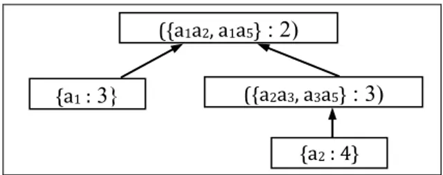
• We insert a first class in the lattice containing the generators of the first column: {a1a2} and {a1a5} having for support 2.
Fig. 5: Lattice after treatment of the first column
• We introduce the second class in the lattice. It corresponds to the second column of the condensed context. It contains the following generators: {a2a3} and {a3a5} and a support = 3.
Besides, because two of these subsets ({a2} ; {a5}) are included in the generators of the first class it becomes the son of the first one.
Fig. 6: Lattice after treatment of the second column
{a1a2 ; a1a5} {a2a3 ; a3a5}
o2 0 1
o3 1 1
o5 1 1
({a1a2, a1a5}
: 2)
({a1a2, a1a5}
: 2)
• Afterward, we start by treating the rest of the generators in increasing order of the support. The list of the rest generators is: {a1:3 ; a2 :4 ; a3 :4 ; a5 :4}.
• Insertion of {a1 :3} in the lattice:
o We compare it with the classes having the same support and if it is not allocated to any one of it, we create a cl ass and we compare it with the classes of lower support to establish the necessary relation between them.
We notice that the class [{a2a3, a3a5} :3] has the same support as the generator to be inserted, then, we verify if the union of {a1} and its generators belongs to GBd +. Because {a1} ∪ {a2a3, a3a5} ≠ GBd+, we create a new class [{a1} :3].
o Afterward, we compare if this generator is included in the generators of the classes of lower support. In our case, a class [{a1a2, a1a5} :2] having a lower support than a new class and {a1} is included in its generators. Then it becomes the parent of the new class.
Fig. 7: Lattice after treatment of {a1:3} • The insertion of {a2 :4}:
o The lattice does not contain any class that has the support 4, we create a new class and we compare it with the generators of three classes of the lattice in decreasing order of the support.
o We begin by comparing {a2} with the class [{a2a3, a3a5} :3], we notice that it is included in its generators then the created class becomes the son of it. The parents of [{a2a3, a3a5} :3] will not be compared to {a2}.
o Comparing [{a2} :3] with the class [{a1} :3]: shows that the inclusion = ∅. In addition {a2} ∪ {a1} (the generator of this class) ∉ GBd+ thus its two classes are incomparable.
Fig. 8: Lattice after treatment of {a2:4} • The insertion of {a3 :4}:
o We compare {a3} with the class [{a1} :4] which has the same support = 4 and we notice that the union of {a3} and its generator ∉ GBd+. Then we create a new class [{ a3} :4].
o Afterward, we compare if this generator is included in the generators of the classes of lower support in decreasing order:
- We verify if {a3} is included in the generators of the class [{a2a3, a3a5}: 3] thus it becomes the son of this class. Therefore, we are not going to compare the parent of this class in {a3}.
- While {a3} is not included in the generator of the class [{a1}: 3], the union {a1} and {a3} ∈ GBd+. This implies that [{a3}: 4] becomes the son of [{a1}: 3].
Fig. 9: Lattice after treatment of {a3 :4} • The insertion of {a5 :4} in the lattice:
The class [{a2} :4] has a support = 4 which is the same as the generator to be inserted. We notice that the union of {a5} and its generators belongs to GBd+ then we add {a5} to this class.
• The insertion of ∅ in lattice:
At the end of the treatment, we insert a class having for generator {∅} and it becomes the son of both classes [{a3}: 4] and [{a2, a5}: 4].
({a1a2, a1a5}
: 2)
({a2a3, a3a5}
: 3)
{a1 :
3}
{a2 :
4}
{a3 :
4}
({a1a2, a1a5}
: 2)
({a2a3, a3a5}
: 3)
{a1 :
3}
{a2 : 4}
({a1a2, a1a5}
: 2)
({a2a3, a3a5}
: 3)
Fig. 10: minimal generators lattice
4.2 Exact and approximative rules extraction
We notice that the principle of this third step is the same as the one presented in the algorithm PRINCE. Indeed, after
the construction of the lattice of generators, we build the lattice of Iceberg containing frequent closed Itemsets associated to every equivalent class according to partial order relation. We use these two lattices to generate the basis of the exact and approximative rules during the third step [3].
Continuation of the example 1:
Having built the lattice of minimal generators, we will construct the lattice Iceberg associated:
Fig. 11: Iceberg lattice
The generic exact associative rules (GBE) and the informative approximative rules (GBA) are presented as follow knowing that a minconf = 0,5.
GBE
Règle Confiance
R1 : a5 a2 1
R2 : a2 a5 1
R3 : a1 a3 1
R4 : a2a3 a5 1
R5 : a3a5 a2 1
R6 : a1a2 a3a5 1
R7 : a1a5
a2a3
1
5. Comparative study
To estimate our method CONDCLOSE, we are going to
compare it with the algorithm PRINCE with regard to the
level of the run time by using four bases of test (benchmark)1, the first two are scattered:
• T40I10D100K is a base containing transactions generated randomly within the framework of a dbQUEST project. It imagines the behavior of the buyers in supermarkets.
• RETAIL: a base of a Belgian hypermarket.
1 http://fimi.ua.ac.be/data/
GBA
Règle Confiance
R8 : a3 a1 0,75 R9 : a3 a2a5 0,75 R10 : a3 a1a2a5 0,50 R11 : a1 a2a3a5 0,66 R12 : a5 a2a3 0,75 R13 : a2 a3a5 0,75 R14 : a5 a1a2a3 0,50 R15 : a2 a1a3a5 0,50 R16 : a2a3 a1a5 0,66 R17 : a3a5 a1a2 0,66
({a2, a5} : 4)
({∅} : 5) ({a3} : 4)
({a1} : 3) ({a2a3}, {a3a5} : 3)
({a1a2}, {a1a5} : 2)
({a2a5} : 4)
({∅} : 5) ({a3} : 4)
({a1a3} : 3) ({a2a3a5} : 3) ({a1a2a3a5} : 2)
{∅}
{a2a3} {a3a5}
{a2} {a5} {a3}
{a1}
While both following ones are dense: • PUMSB contains statistical data.
• MUSHROOM contains the characteristics of diverse sorts of mushrooms.
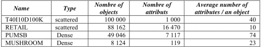
The table (Table 1) contains their main characteristics: the name, the type (dense, scattered), the number of objects, the number of attributes as well as the average number of attributes associated to an object.
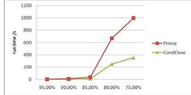
5.1 Comparative study by using the scattered bases
In this section, we are going to present the influence of both scattered bases: T40I10D100K and RETAIL on the global processing time of CONDCLOSE and PRINCE.Afterward, we are going to compare their run time by varying the values of supports in the case of every base. As shown in table (Table 1), the base T40I10D100K is characterized by a high number of objects (100 000) and the average number of attributes associated to an object (40). Consequently, we observe that the first step of CONDCLOSE is the most expensive with regard to the
processing time of the second and the third step. This is due to the number of the minimal generators which increases when we minimize the support.
During the first step, the calculation time of the supports of the minimal generators is smaller than the time generated by PRINCE. This is due to the fact that CONDCLOSE uses
pseudo contexts to determine the candidate generators and eliminate the non frequent generators while PRINCE bases
himself on the initial context during all the treatment of this step.
During, the second step, the condensed context and the positive border (GBd+) generated in the first step of CONDCLOSE plays an important role in the minimization of
the processing time.
We also notice that the construction of the Iceberg lattice and the extraction of the generic exact and approximative rules are systematic from the lattice of the minimal generators in the case of the base T40I10D100K and the base RETAIL. This implies a low processing time of the third step of both algorithms in the case of both bases.
Fig. 12: The run time of PRINCE and CONDCLOSE at different minimum
support levels on T40I10D100K
Indeed, according to the table (Table 1), RETAIL contains a high number of objects (88 162) and the average number of attributes associated to an object (10), which explains that it is scattered. The processing time of the first step of CONDCLOSE is reduced because of the use of pseudo
contexts during the extraction of the minimal generators. We also notice that the condensed context and the small size of the positive border (GBd+) make a reduced time of the second step with regard to PRINCE.
Fig. 13: The run time of PRINCE and CONDCLOSE at different minimum support levels on RETAIL
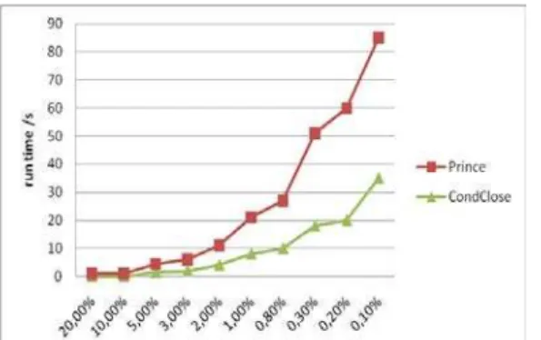
5.2 Comparative study by using the dense bases
This section contains an analysis of the impact of the characteristics of two bases: PUMSB and MUSHROOM on the processing time of both algorithms CONDCLOSE andPRINCE.
Indeed, the reduced number of objects and the average number of attributes associated to an object (74) characterize the base PUMSB. The calculation of the supports of the candidate generators by using all the base every time is the major handicap of the algorithm PRINCE.
While the use of the pseudo contexts by CONDCLOSE,
which is a compact structure containing only the k-minimal generators used to determine the (k+1)-candidate generators is an important means of reduction of the calculation time of support and thus of the first step. We observe that the second and the third step have no significant influence on the run time of CONDCLOSE and
Fig. 14: The run time of PRINCE and CONDCLOSE at different minimum
support levels on PUMSB
In fact, in the case of the MUSHROOM, the reduced number of objects as well as the average number of attributes associated to an object make a minimum time of treatment of the first step in the case of both algorithms. However, with a high support, the number of minimal generators becomes low and because PRINCE treats the
notion of negative border (GBd-) which have a high size. This latter make a long time of research during the construction of the minimal generators lattice.
As for CLOSECOND which treats the positive border
(GBd+) that has a l ower size than the negative border (GBd+) which implies a lower cost of the second step with regards to that of PRINCE.
The third step does not influence the global processing time of both algorithms in the tests, with PUMSB and with MUSHROOM.
Fig. 15: The run time of PRINCE and CONDCLOSE at different minimum support levels on MUSHROOM
5. Conclusion
With the aim of reducing the processing time of extraction of associative rules and improving the quality of the extracted knowledge, we presented a n ew method called CONDCLOSE based on the notion of condensed context
allowing to build a structure partially ordered by frequent minimal generators which will be used, afterward, to determine the generic base of associative rules.
We notice that the reduction of the size of the initial context in every iteration of extraction of k-generators by building pseudo contexts which contains only these last ones as well as their associated objects, minimizes the time of the treatment and more exactly the time of the self-joint and that of the elimination of non frequent generators. Besides, the use of the condensed context which is the result of the first step to build the lattice facilitates the definition of the elements of every equivalent classes and the relation of inclusion between them.
So, our method allows to transform the scattered contexts into small-sized dense contexts to minimize the number of candidate generators and reduce the calculation time of the support.
Acknowledgments
My special thanks go to Mrs. Ahlem Dababi Zwawi for her help to translate this paper from French to English.
References
[1] Agrawal R., Imielinski T. and Swami A. N., “Mining association rules between sets of items in large databases”, In Proceedings of the International Conference on Management of Data, ACM SIGMOD’93, Washington, D.C., USA, page 207-216, May 1993.
[2] Agrawal R. and Srikant R., “Fast algorithms for mining association rules”, In J. B. Bocca, M. Jarke and C. Zaniolo, editors, Proceedings of the 20th International Conference on Very Large Databases, Santiago, Chile, p.p. 478-499, June 1994.
[3] Bastide Y., Pasquier N., Taouil R., Lakhal L. and Stumme G., “Mining minimal non-redundant association rules using frequent closed itemsets”, Proceedings of the Intl. Conference DOOD’2000, LNCS, Springer-verlag, July 2000, p. 972-986.
[4] Ben yahia S., Latiri C., Mineau G.W. and Jaoua A., “Découverte des règles associatives non r edondantes – application aux corpus textuels”, In M.S. Hacid, Y. Kodrattof and D. Boulanger, editors EGC, volume 17 of Revue des Sciences Technologies de l’Information – série RIA ECA, pages 131-144. Hermes Sciences Publications, 2003.
[5] Brin S., Motwani R., Ullman J.D. and Tsur S., “Dynamic itemset counting and implication rules for market basket data”, In : Proceedings ACM SIGMOD International Conference on Management of Data, Tucson, Arizona, USA, éd. par Peckham (Joan). pp. 255-264 - ACM Press, 1997.
[6] Cheung W., Heung W. and Zaiane O., “Incremental Mining of Frequent Patterns Without Candidate Generation or Support Constraint”, Proceedings of the Seventh International Database Engineering and Applications Symposium (IDEAS 2003), Hong Kong, China, July 2003.
[7] Ganter B. and Wille R., “Formal Concept Analysis”, Mathematical Foundations, Springer, 1999.
[8] Han J., Pei J. and Yin Y., “Mining frequent patterns without candidate generation”, CM-SIGMOD Int. Conf. on Management of Data, pp. 1-12, Mai 2000.
[9] Hamrouni T., Ben Yahia S. and Slimani Y., “Prince: An algorithm for generating rule bases without closure computations”, In 7th International Conference on Data Warehousing and Knowledge discovery (DaWaK’05), pages 346-355, Copenhagen, Denmark, 2005. Springer-Verlag, LNCS.
[10] Kruse R. L. and Ryba A. J., “Data structures and program design in c++”, Prentice Hall, 1999.
[11] Liu G., Li J. and Wong L., “A new concise representation of frequent Itemsets using generators and a positive border”, Knowledge and Information Systems, 17(1) : 35-56, 2008.
Lattices”, Information Systems Journal, vol. 24, no 1, 1999, p. 25-46.
[13] Pei J., Han J., Mao R., Nishio S., Tang S. and Yang D., “CLOSET : An efficient algorithm for mining frequent closed Itemsets”, Proceedings of the ACM SIGMOD DMKD’00, Dallas, TX, 2002, p. 21-30.
[14] Savasere A., Omiecinsky E. et Navathe S., “An efficient algorithm for mining association rules in large databases”, 21st Int'l Conf. on Very Large Databases (VLDB), Septembre 1995.
[15] Stumme G., Taouil R., Y. Basride, N. Pasquier and L. Lakhal, “Computing Iceberg Concept Lattices with TITANIC”, J. on Knowledge and Data Engineering (KDE), vol. 2, no 42, 2000, p. 189-222.
[16] Zaki M., Parthasarathy S., Ogihara M. and Li W., “New algorithms for fast discovery of association rules”, In : 3rd Intl. Conf. on Knowledge Discovery and Data Mining, éd. par Heckerman (D.), Mannila (H.), Pregibon (D.), Uthurusamy (R.) et Park (M.). pp. 283-296. AAAI Press, 1997.
[17] Zaki M. and Hsiao C. J., “CHARM : An Efficient Algorithm for Closed Itemset Mining”, Proceedings of the 2nd SIAM International Conference on Data Mining, Arlington, April 2002, p. 34-43.
First Author Hamida Amdouni received her Master degree in Computer Science at FST-Tunisia in 2005. Now, she prepared her PhD at the Faculty of Sciences of Tunis. Her main research contributions concern: data mining, Formal Concept Analysis
(FCA) and Customer Relation Management. She is member of Research Laboratory RIADI
Second AuthorMohamed Mohsen Gammoudi is currently an Associate Professor at the Engineering School of Statistics and Data Analysis. He is member of Research Laboratory RIADI. He obtained his habilitation to Supervise research in 2005 at the Faculty of Sciences of Tunis. He got his PhD in September 1993 in Sophia Antipolis Laboratory I3S/CNRS in the team of Professor Serge Miranda. In 1989, He received his Master degree in computer Sciences at LIRM laboratory of Montpellier, France. He succeeded his graduate degree in computer sciences at the University of Aix Marseille II during 1986-1988. Professor Gammoudi’s professional work experience began in 1992 when he was assigned as an assistant at the Technical University of Nice. Then he was hired as a visiting professor between 1993 and 1997 at Federal University of Maranhao, Brazil. He was the head of research group in this university during that period. In November 1997, he was Senior Lecturer at the Faculty of Sciences of Tunis. Since, he supervised several PhD and master thesis. In 2005 he served as Lecturer and w orked at the Higher Institute for Computer Sciences and Management of Kairouan, Tunisia.
Table 1: Characteristics of the bases of test
Name Type Nombre of
objects
Nombre of attributs
Average number of attributes / an object
T40I10D100K scattered 100 000 1 000 40
RETAIL scattered 88 162 16 470 10
PUMSB Dense 49 046 7 117 74