DOI 10.1007/s11760-007-0027-2 O R I G I NA L PA P E R
Decision directed adaptive blind equalization based on the constant
modulus algorithm
Carlos Alexandre R. Fernandes · Gérard Favier · João Cesar M. Mota
Received: 7 August 2006 / Revised: 7 June 2007 / Accepted: 8 June 2007 / Published online: 4 July 2007 © Springer-Verlag London Limited 2007
Abstract In this paper, new decision directed algorithms for blind equalization of communication channels are pre-sented. These algorithms use informations about the last decided symbol to improve the performance of the constant modulus algorithm (CMA). The main proposed technique, the so called decision directed modulus algorithm (DDMA), extends the CMA to non-CM modulations. Assuming correct decisions, it is proved that the decision directed modulus (DDM) cost function has no local minima in the combined channel-equalizer system impulse response. Additionally, a relationship between the Wiener and DDM minima is estab-lished. The other proposed algorithms can be viewed as mod-ifications of the DDMA. They are divided into two families: stochastic gradient algorithms and recursive least squares (RLS) algorithms. Simulation results allow to compare the performance of the proposed algorithms and to conclude that they outperform well-known methods.
Keywords Blind equalization·CMA·Decision directed·Stochastic gradient·RLS
C. A. R. Fernandes·G. Favier (
B
)I3S Laboratory, CNRS, University of Nice-Sophia Antipolis, Les Algorithmes/Euclide B, 2000 route des Lucioles, BP 121, 06903 Sophia-Antipolis Cedex, France e-mail: favier@i3s.unice.fr
C. A. R. Fernandes e-mail: acarlos@i3s.unice.fr J. C. M. Mota
Wireless Telecommunication Research Group (GTEL), Federal University of Ceará, Campus do Pici, 60.755-640, 6007 Fortaleza, Brazil
e-mail: mota@deti.ufc.br
1 Introduction
the equalizer is done by the CMA. This equalization scheme, called the CMA–DDMA, provides an improved robustness to ISI in relation to the CMA–DDA one.
The analysis of the DDMA is initially focused on the study of its stationary points, by exploiting an expansion of its cost function in the case of QAM signals, assuming that the deci-sion device takes right decideci-sions, i.e. the decided symbol is equal to the transmitted symbol with a fixed delay. Then, the behavior of the DDMA for real valued signals is analyzed by establishing a relationship between the DDM and Wiener criteria.
Another stochastic gradient algorithm based on the same approach as the DDMA is proposed. This algorithm that can be viewed as a generalization of the modified constant mod-ulus algorithm (MCMA) [13,14], is called the modified deci-sion directed modulus algorithm (MDDMA). That leads to a family of four stochastic gradient algorithms. Then, we derive recursive least squares (RLS) versions of the previ-ous algorithms. These algorithms are based on least squares versions of the CM and DDM cost functions. This family of RLS algorithms provides better performances at the cost of an increased computational complexity.
The rest of the paper is organized as follows. Section2 introduces the mathematical model used in this work. Section3revisits the original CMA. In Sect.4, the DDMA is introduced. In Sect.5, we make a theoretical analysis of the DDMA. Section6presents in an unified way the two fam-ilies of stochastic gradient and RLS algorithms. In Sect.7, we compare the performance of the proposed algorithms by means of simulations. Some conclusions are drawn in Sect.8.
2 Mathematical model
The linear single-input-single-output (SISO) discrete-time baseband equivalent communication model considered in this work is shown in Fig.1. Let us assume that the indepen-dently and identically-distributed (i.i.d.) transmitted sequence{a(n)}can take the value of any constellation sym-bol with equal probability. The received signal is expressed as:
x(n)= N−1
i=0
hia(n−i)+v(n)=hTa(n)+v(n), (1)
wherea(n)= [a(n) a(n−1) · · · a(n−N+1)]T,h =
[h0 h1 · · · hN−1]T is the vector of the impulse response of the time-invariant moving-average (MA) channel,N is the channel length andv(n)is an additive white gaussian noise (AWGN). The output of the equalizer can be written as:
y(n)= M−1
i=0
wix(n−i)=wTx(n)=fTa˘(n)+wTv(n),
(2)
wherew= [w0w1 · · · wM−1]T is the vector of the impulse response of the equalizer, M is the number of taps of the equalizer andx(n)= [x(n)x(n−1)· · ·x(n−M+1)]T is its regression vector. Moreover, we havea˘(n)= [a(n)a(n− 1) · · · a(n−N−M+2)]T,v(n)= [v(n)v(n−1)· · ·v(n−
M +1)]T and f = HTw ∈ C(N+M−1)×1, wheref is the
combined channel-equalizer impulse response andHis the channel matrix:
H= ⎛
⎜ ⎜ ⎜ ⎝
h0h1· · ·hN−1 0 · · · 0
0 h0 h1 · · · hN−1· · · 0 .
.
. . .. . .. . .. . .. ...
0 0 · · · h0 h1 · · ·hN−1
⎞
⎟ ⎟ ⎟ ⎠
∈CM×(N+M−1). (3)
We denote byaˆ(n)=Dec[y(n)]the output of the decision device, i.e. the estimated symbol. The structure shown in Fig.1may also include a phase-locked loop (PLL) between the equalizer and the decision device to correct any phase shift.
3 The constant modulus algorithm
The constant modulus algorithm (CMA), developed by Godard [1] and Treichler [2], is one of the most classical techniques to perform blind equalization. Its cost function is defined as:
JCM=E{(Rp− |y(n)|p)2}, with Rp=
E{|a(n)|2p} E{|a(n)|p}, (4) where E{·}denotes the expectation operation. In this paper, we consider the casep=2, that is also referred to as “CMA 2-2” by some authors. The CMA is derived by using the sto-chastic gradient of its cost function, which leads to the fol-lowing equation for adapting the equalizer tap-weight vector:
w(n+1)=w(n)+µy(n)(R− |y(n)|2)x∗(n), (5)
Fig. 1 Simplified structure of a communication system
Channel + Equalizer
v(n)
a(n) x(n) y(n)
h
Dec[ • ] â(n)
w
equation given by: w(n+1)=w(n)+µ
ˆ
a(n)−y(n) x∗(n). (6)
4 The decision directed modulus algorithm
In this section, we present a new algorithm, called the decision-directed modulus algorithm (DDMA), designed to improve the performance of the CMA and the DDA, in terms of convergence speed and steady-state error. This algorithm can be viewed as a generalization of the CMA for multiple radii constellations. The DDM cost function uses the squared magnitude of the decided symbolaˆ(n)and is defined as: JDDM =E{(| ˆa(n)|2− |y(n)|2)2}. (7) Taking the stochastic gradient of (7), we obtain the following DDMA adaptation equation:
w(n+1)=w(n)+µy(n)(| ˆa(n)|2− |y(n)|2)x∗(n). (8) The derivative ofaˆ(n)with respect towwas assumed to be zero, since the value ofaˆ(n)does not vary for an infinitesi-mal variation inw. The DDMA can be viewed as a version of the CMA with a variable reference modulus. It is easy to see that the DDMA and CMA are equivalent for PSK modu-lations. However, for high-level QAM constellations, when perfect equalization is achieved, the correction term of the DDMA adaptation equation (8) goes to zero while with CMA it does not. This “constellation matched” nature of the DDM cost function allows to improve the performance, in terms of convergence speed and steady-state error, of the DDMA in relation to the CMA for QAM constellations, as will be illustrated by simulation results in Sect.7.
However, as the DDMA uses an information about the last decided symbol, its performance can be degraded if the num-ber of incorrect decisions is too large. To solve this problem and improve the stability of the algorithm, the initial adjust-ment of the tap weight vector can be done by the CMA and when some switching criterion is achieved, the equalization algorithm switches to the DDMA. This algorithm will be calleddual-mode DDMAor CMA–DDMA. The switching criterion used in the simulations will be described later in the paper.
It should be highlighted that the DDM cost function uses only the magnitude of the decided symbol, which implies that it is invariant to phase-shifts, if these phase-shifts do not
change the magnitude of the decided symbol. This character-istic provides to the DDMA a greater robustness to imperfect carrier recovery than that of the DDA. An incorrect decision can be viewed by the DDMA as a “correct decision” when the incorrect decided symbol has the same magnitude than the correct symbol. Thus, the number of “decision regions” of the DDMA is smaller than the number of constellation points. For example, with 16QAM and 64QAM signals, while the DDA takes a decision among 16 and 64 symbols respectively, the DDMA takes a decision among only 3 and 9 different amplitudes respectively. As a result, the DDMA has a greater robustness to ISI than the DDA. The simulation results will confirm that the dual mode algorithm CMA–DDMA has a better robustness to ISI than the traditional scheme CMA– DDA.
Other authors proposed generalizations of the CM cost function for multi-moduli constellations. In [15,16], the pro-posed CMA-based algorithms are also driven by previous decisions, but the decision is made from the modulus of the equalizer output and the nearest symbol radius. This means that, even if the output of the equalizer is inside the deci-sion region of the desired symbol, its modulus may be closer to the radius of another constellation symbol. This fact may affect the performance of the algorithm, specially for high level QAM signals. Other works have proposed algorithms based on the CMA. Among them we may cite [17,18], that use dual-mode CM-based cost functions to improve the per-formance of the CMA. However, these works deal with cost functions with a high computational complexity compared with that of the CM. That leads to algorithms much more complex than the CMA, unlike the DDMA, which improves the performance of the CMA with a very similar complexity.
5 Analysis of the DDMA
In this section, we make a theoretical analysis of the DDMA. It is assumed that the decision device takes correct decisions, i.e. the decided symbol is equal to the transmitted symbol a(n−τ ). In this case, we haveaˆ(n)=a(n−τ ), whereτ ∈ [0,1,…,N+M−2] is a fixed transmission delay.
5.1 Stationary points of the DDM cost function
We assume that the transmitted signal is circular of order 2, i.e. E{a2(n)} =0, with a uniform and non constant modu-lus QAM constellation. As already mentioned, in the case of constant modulus modulations, the DDM and CM cost func-tions are equivalent and, in this case, it was demonstrated that the zero-forcing (ZF) solution is the only minimum in the spacef[19].
The next theorem provides all the stationary points of the DDM cost function by making the hypothesis of correct deci-sions.
Theorem 1 Assuming that the decided symbol is equal to the transmitted symbol a(n −τ ), for a circular, uniformly distributed and non constant modulus QAM constellation, in a noiseless environment, the only minimum of the DDM cost function in the combined channel-equalizer system impulse response space is the ZF solutionf=eτ= [0 0· · ·1· · ·0]ejϕ,
for0≤τ ≤N+M−2, whereeτ is theτt h canonical unit
vector,τ denoting a fixed decision delay andϕan arbitrary phase shift.
Proof Ifaˆ(n) =a(n−τ ), we may rewrite the DDM cost function in the following way:
JDDM =E{(|a(n−τ )|2− |y(n)|2)2}. (9) After some algebraic manipulations, the DDM cost function (9) can be expanded as:
JDDM =(m4a−2σa4) N+M−2
i=0
|fi|4+2σa4
N+M−2
i=0 |fi|2
2
−2m4a|fτ|2−2σa4 N+M−2
i=0,i=τ
|fi|2+m4a, (10)
where E{|a(n)|4} =m4aand E{|a(n)|2} =σa2. The station-ary points of the DDM cost function are obtained by setting to zero the gradient of (10) with respect tof:
∇fJDDM(k)=2 ∂JDDM
∂fk∗
=4fk ⎛
⎝m4a|fk|2+2σa4 N+M−2
i=0,i=k
|fi|2−σa4 ⎞
⎠=0
(11) fork=τ, and:
∇fJDDM(τ )=2 ∂JDDM
∂f∗
τ
=4fτ
⎛
⎝m4a|fτ|2+2σa4 N+M−2
i=0,i=τ
|fi|2−m4a ⎞
⎠=0,
(12) where 0≤k≤N+M−2 and∇fJDDM(k)denotes thekth component of the gradient vector∇fJDDM. Thus, the solu-tions of (11) and (12) correspond to the stationary points of
the DDM cost function. It is easy to verify that the null vector of dimensionN+M −1, i.e.f=0N+M−1, is a trivial sta-tionary point. In the sequel, it will be proved that if another vector satisfies (11) and (12), then all its nonzero compo-nents have the same magnitude, except fτ. To do so, let us
consider two different nonzero components satisfying (11) fl =0 and fk=0 such thatl=k. Then, we have:
m4a−2σa4
|fl|2=
m4a−2σa4
|fk|2⇒ |fl|=|fk|, (13)
which proves that all the components fk =0 (k=τ) have the same magnitude. We denoteNM(0≤ NM ≤N+M−2) the number of nonzero components fk of the vectorfsuch thatk=τ. Now we prove that (11) and (12) admit solutions only ifNM =0 orNM =1.
By using the equality (13), we may rewrite (11) and (12), for fk =0, fτ =0 andk=τ, as:
m4a|fk|2+2σa4
(NM −1)|fk|2+ |fτ|2
=σa4, (14) m4a|fτ|2+2σa4NM|fk|2=m4a. (15)
The solution of (14) and (15) is given by:
|fτ|2=
2σ8
aNM−m4a[m4a+2σa4(NM −1)] 4σ8
aNM−m4a[m4a+2σa4(NM −1)]
, (16)
|fk|2=
m4aσa4 4σ8
aNM−m4a[m4a+2σa4(NM −1)]
, k=τ.
(17)
In Appendix A, it is shown that if the transmitted signal a(n)has a uniform non constant modulus QAM distribution, then (16) exists only forNM =0 orNM =1.
The above result allows us to separate the possible nonzero stationary points of the DDM cost function in two categories:
• NM = 0: In this case, we have|fτ|2 =1 and|fk|2 = 0,k = τ. This solution corresponds to the ZF solution given byf=eτ = [0 0· · ·1· · ·0]ejϕ, whereϕis a phase
shift. With no loss of generality it can be assumed that ϕ=0, since the phase shift can always be suppressed by a PLL.
• NM =1: In this case, we have:
|fτ|2=
2σa8−m24a 4σ8
a−m24a
and |fk|2=
σa4m4a
4σ8 a−m24a
, k=τ.
(18)
may write:
m42a> σa8⇒σa4m4a+m24a>2σa8⇒σa4m4a>2σa8−m24a. (19) From (18) and (19), it follows that|fk|>|fτ|. Let us define
a parameter that measures the “amount”of ISI at the receiver, considering a fixed transmission delay equal toτ:
ISIτ =
N+M−2
i=0 |fi| − |fτ|
|fτ|
, (20)
In the case of the solution (18), we get ISIτ = ||ffkτ|| > 1.
When ISIτ ≥ 1, the channel eye is said to be closed and
there is a high probability of decision error. That means that the solution (18) is not a stationary point of the DDM cost function under the considered assumptions.
Therefore, the DDM cost function admits only two solu-tions, the zero vector f = 0N+M−1 and the ZF solution f = eτ. In order to determine the global minimum of the
DDM cost function, the expressions of the Hessian matrix of JDDM at the pointsf = 0N+M−1andf =eτ are
devel-oped in Appendix B. From the expressions (B.4) and (B.5), it can be concluded that the pointf =0N+M−1 is a maxi-mum (∇2J
DDM(f =0N+M−1) <0) and thatf= eτ is the
global minimum (∇2JDDM(f=e
τ) >0) of the DDM cost
function. ⊓⊔
5.2 Additional comments on convergence
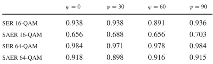
We have to notice that, in the cost function (9), only a relaxed assumption (that the amplitude of the decided symbol is equal to the amplitude of the transmitted symbol) is used. The strong assumption (that the decision is correct) is needed only to conclude that in the caseNM =1 the solution (18) does not correspond to a stationary point of the DDM cost function. Even in that case, the relaxed assumption can be sufficient as it is illustrated in Table1that shows the symbol error rate (SER) and the symbol amplitude error rate (SAER) for uniformly distributed 16-QAM and 64-QAM signals. The SAER is defined as the rate between the number of symbols for which the magnitude of the decided symbolaˆ(n)is dif-ferent from the magnitude of the symbola(n−τ ), and the total number of symbols. For uniformly distributed 16-QAM and 64-QAM, using the solution (18), we get respectively |fτ| =0.338,|fk| =0.765 and|fτ| =0.211,|fk| =0.812. With no loss of generality it can be assumed that fτ = |fτ|
and fk = |fk|ejϕ, since the phase shift of fτ can be
sup-pressed by a PLL. The values of the SER and SAER shown in Table1were calculated for fixed and known values ofτ andk, and four different values ofϕ. This result indicates that the solution (18) also violates the hypothesis of correct amplitude decisions associated with the delayτ.
The assumptions of correct decisions or correct amplitude decisions may seem unrealistic. However, the dual-mode
Table 1 SER and SAER provided by the solution (18)
ϕ=0 ϕ=30 ϕ=60 ϕ=90
SER 16-QAM 0.938 0.938 0.891 0.936
SAER 16-QAM 0.656 0.688 0.656 0.703
SER 64-QAM 0.984 0.971 0.978 0.984
SAER 64-QAM 0.918 0.898 0.916 0.915
version of the DDMA is designed in order to make these assumptions valid. In this scheme, the DDMA acts when the hypothesis of correct decisions is roughly verified. Another approach to eliminate the effect of incorrect decisions con-sists in using a short training period, during which the decided symbolaˆ(n)is replaced bya(n−τ )in the adaptation equa-tion (8). In this semi-blind scheme, the DDMA acts at the end of the acquisition mode and in the tracking mode. Although the above mathematical analysis is valid under the hypothe-sis of correct decisions, simulations showed that the DDMA almost always converges towards the global minimum if the number of incorrect amplitude decisions is not too high.
Moreover, the analysis of the stationary points was done in the combined channel-equalizer system impulse response space. In practice, this space is not accessible. In [20], it was demonstrated that the stationary points in this space and in the equalizer impulse response space are equivalent if and only if the channel matrix H has a trivial nullspace. This happens for flat fading channels or for doubly-infinite param-eterized equalizers. In a multichannel system, it is also pos-sible, under certain conditions, to choose the length of the equalizer in such a way that the nullspace ofHis trivial [21]. Other related works about the convergence of adaptive blind algorithms can be found in [22–28].
5.3 Relationship between the DDM and Wiener cost functions: case of real valued signals
The following developments are inspired on the works [29,30], where the authors have derived similar results for the CM and Wiener criteria. For any real valued signals, the DDM cost function can be written as:
JDDM(w)=E{[y(n)− ˆa(n)]2[y(n)+ ˆa(n)]2}, (21)
withy(n)=wTx(n). By using the Cauchy–Schwarz inequal-ity and assuming that the decision device takes right deci-sions, i.e.,aˆ(n)=d(n)=a(n−τ ), we get:
JDDM(w)≤JLMF(w)JLMF(−w), (22)
whereJLMF(w)=E{[y(n)−d(n)]4} =E{e4(n)}is theleast mean fourth(LMF) cost function andd(n)is the desired sig-nal.
The equality in (22) holds ifw=0M, sinceJLMF(0M)=
the equality also holds forw = wWiener, with an appropri-ate delayτ for whichJDDM(wWiener)=JLMF(wWiener)=0. The distance between the two level curves associated with the two members of (22) becomes small at the points close to the Wiener minimum and it takes high values at the points corre-sponding to a bad equalization. So, the inequality (22) can be rewritten as an approximate equality valid in the neighbor-hood of the Wiener solution. In this neighborneighbor-hood, it is rea-sonable to assume that the Wiener cost function takes small values, in such a way that we have the following approxi-mationE{e2(n)}2=∼E{e4(n)}[30], which leads to the fol-lowing relationJLMF(w)∼= JWiener2 (w), where JWiener(w) = E{[y(n)−d(n)]2} =E{e2(n)}is the Wiener cost function. So, we get the following approximation for the DDM cost function in the neighborhood of the Wiener solution:
JDDM(w)∼=JWiener(w)JWiener(−w). (23)
Equation (23) gives a relationship between the DDM and Wiener cost functions, valid in the neighborhood of the Wiener minimum. An illustration of the relationship (23) is provided by Fig.2that shows the level curves of the DDM cost function, assuming right decisions associated with the delayτ =2, for a noiseless channel with an impulse response given byh = [0.4 1]T. The considered equalizer has two real-valued taps and the transmitted signal is a 4-PAM (pulse amplitude modulation). The black marks in this figure show the points where the difference between the DDM cost func-tion and its approximafunc-tion (23) is smaller than 10−2. It can be verified that the approximation is good in the neighborhood of the points±wWiener = ±[−0.337 0.978]T.
Taking the gradient of (23) equal to zero, we get:
∇wJDDM ∼=4RxwADDM(w
T
ADDMRxwADDM) +4RxwADDMσ
2
d−8pdx(wADDMT pdx)=0M, (24)
−1 −0.8 −0.6 −0.4 −0.2 0 0.2 0.4 0.6 0.8 1
−1 −0.8 −0.6 −0.4 −0.2 0 0.2 0.4 0.6 0.8 1
w1
w0
Fig. 2 DDM cost function
whereRx =E{x(n)x(n)T}is the autocorrelation matrix of the received signal x(n),σd2 is the variance of the desired signal d(n),pdx =E{d(n)x(n)}is the cross-correlation vec-tor betweenx(n)andd(n), andwADDM is the approximate DDM (ADDM) minimum. Pre-multiplying the two mem-bers of this equation byR−x1and using the Wiener solution wWiener=R−x1pdx, we get:
wWiener=
wTADDMRxwADDM +σ 2 d 2wT
ADDMpdx
wADDM, (25)
which links the Wiener and ADDM solutions. Moreover, it explicitly points out the collinearity of these two solutions. The quotient factor in the right side of (25) is associated with the distance between wWiener andwDDM. The relationship (25) will be validated later in the paper by means of simula-tion results showing that this quotient factor can be close to unity. The same expressions (23) and (25) were developed in [30] for the CM and Wiener cost functions, but restricted to the case of 2-PAM signals.
6 Other DDM-based algorithms
In this section, the decision directed modulus approach is used to develop a new family of stochastic gradient algo-rithms, as well as a family of RLS-type algorithms. The key point consists in using the last decided symbol in the cost functions to be minimized.
6.1 A family of stochastic gradient algorithms
Oh and Chin [13], and Yang et al. [14] proposed the modi-fied constant modulus algorithm (MCMA), also called mul-timodulus algorithm (MMA) [14]. The MCM cost function, given in Table2, is based on a decomposition of the CM cost function, and the corresponding adaptation equation can be written as:
w(n+1)=w(n)+µe1(n)x∗(n), (26)
wheree1(n)is also given in Table2.yR(n)andyI(n)denote, respectively, the real and imaginary parts ofy(n);RRandRI are constants given by RR =
E{aR4(n)}
E{aR2(n)} and RI =
Table 2 The family of CMA-type algorithms
Algorithms Cost functions e1(n)
CMA E{(R− |y(n)|2)2} y(n)(R− |y(n)|2)
DDMA E{(| ˆa(n)|2− |y(n)|2)2} y(n)(| ˆa(n)|2− |y(n)|2)
MCMA E{(RR−yR2(n))2 +(RI−y2I(n))2} yR(n)(RR−yR2(n))+j yI(n)(RI−yI2(n))
MDDMA E{(aˆR2(n)−yR2(n))2 +(aˆI2(n)−y2I(n))2} yR(n)(aˆR2(n)−yR2(n))+j yI(n)(aˆI2(n)−yI2(n))
Table 3 The family of RCMA-type algorithms
Algorithms Cost functions e2(n)
RCMA ni=0λn−i(R− |y(i)|2)2 ξ(n)(R− |ξ(n)|2)
RDDMA ni=0λn−i(| ˆa(i)|2− |y(i)|2)2 ξ(n)(| ˆa(n)|2− |ξ(n)|2)
RMCMA ni=0λn−i
(RR−y2R(i))2 +(RI−yI2(i))2
1
ξ(n)
ξR(n)(RR−ξR2(n))+jξI(n)(RI−ξI2(n))
RMDDMA ni=0λn−i
(a2
R(i)−yR2(i))2 +(aI2(i)−yI2(i))2
1
ξ(n)
ξR(n)(aR2(n)−ξR2(n))+jξI(n)(aˆ2I(n)−ξI2(n))
It is possible to combine the modifications brought to the CMA by the DDMA and the MCMA to get a new tech-nique that incorporates the improvements of both algorithms, which leads to the modified decision directed modulus algo-rithm (MDDMA). Its cost function is also shown in Table2, and its adaptation equation is the same as (26) withe1(n) given in Table2. The indices R and I inaˆR(n)andaˆI(n) denote, respectively, the real and imaginary parts of the decided signalaˆ(n). This algorithm can be viewed as a “mod-ified” version of the DDMA and it is potentially capable of outperforming the CMA, MCMA and even the DDMA, in terms of residual error and/or convergence speed.
However, the MDDMA being decision directed, its per-formance deteriorates if the number of incorrect decisions is too large. To improve its stability, it is possible to use the same dual-mode scheme introduced earlier. In this case, due to the similarity of its adaptation equation, the MCMA performs the initial adjustment of the equalizer. In the next section, simulation results will show that the dual-mode algo-rithm MCMA–MDDMA has a better performance than the dual-mode algorithms CMA–DDA and CMA–DDMA.
6.2 A family of RLS algorithms
The recursive constant modulus algorithm (RCMA), pro-posed in [32,33], provides a fast blind algorithm at the expense of an increased complexity. A least squares ver-sion of the CM cost function, expressed in Table3, where y(i) = wTx(i)and 0 < λ ≤ 1 is the forgetting factor, is minimized using some approximation. The RCMA is sum-marized by the following equations:
k(n)= P(n−1)s ∗(n)
λ+s⊤(n)P(n−1)s∗(n), where s(n)=ξ
∗(n)x(n),
(27)
P(n)=λ−1·P(n−1)−k(n)s⊤(n)P(n−1), (28) w(n)=w(n−1)+k(n)e2(n), (29) wheree2(n)is given in Table3,ξ(n)=wT(n−1)x(n)is the a priori equalizer output andP(n)is a matrix initialized as P(0)=δIM,δbeing a positive constant andIM the identity matrix of orderM.
adaptation equations are proved in Appendix C. They are summarized by (27–29), withe2(n)given in Table3. As it will be illustrated by computer simulations, the RMCMA provides very good performances, notably improving the convergence speed of the original CMA. Moreover, the RMCMA being not decision directed, it is not affected by incorrect decisions. The decomposition of its cost function in real and imaginary terms makes the RMCMA more adapted to squared constellations than the RCMA.
It is also possible to combine the modifications brought by the RDDMA and RMCMA. That leads to the recursive mod-ified decision directed modulus algorithm (RMDDMA), the cost function of which is also given in Table3. This algorithm is described by (27–29), withe2(n)given in Table3. It can be viewed as a generalization of the RMCMA with variable reference radii. For high order QAM signals, when perfect equalization is achieved, the estimation error of the RMD-DMA goes to zero, while it is not the case for the RMCMA. As a result, the RMDDMA provides the best performance between all the methods studied in this work, if there is not a large number of incorrect decisions, as it will be illustrated by computer simulations. The RMDDMA can also be used in a dual-mode approach, with the RMCMA operating as the initial algorithm.
7 Simulation results
In this section, the performance of the proposed algorithms is illustrated by means of simulations. The equalizers are ini-tialized with a single non-zero middle tap equal to 1 (center-tap initialization) and the horizontal line in the MSE figures corresponds to the Wiener MSE. The results were obtained via Monte Carlo simulations using 50 independent data real-izations. In order to accentuate the averaging effect in the curves, the MSE values were passed through a low-pass fil-ter of order equal to 2 and with a cut-off frequency equal to 10−2, before ploting.
The dual-mode algorithms use a switching factor that con-trols a soft transition between two criteriaJ1andJ2, so that, at iterationn, the criterion to be minimized isJ=α(n)J1+ (1−α(n))J2, where J1 is a robust cost function, i.e. not decision directed,J2is a DDM-based cost function,α(n)= (tanh|eDD(n)|)2,eDD(n)= y(n)− ˆa(n)for the CMA-type algorithms andeDD(n)=ξ(n)− ˆa(n)for the RCMA-type algorithms. The only exception is Fig.4, where a hard switch-ing between the two algorithms was used when the number of iterations is equal to an a priori fixedswitching number(SN). To compare the performance of the algorithms, the step-size parameterµis adjusted in such a way that all the algo-rithms provide approximately the same steady-state error. When there is some problem of convergence, the step size was simply chosen so that a good tradeoff between conver-gence speed and residual MSE is achieved.
7.1 Stochastic gradient algorithms
The first simulation scenario consists in a transmitted signal with a 16QAM or 64QAM modulation, an equalizer with nine taps, a signal-to-noise-ratio (SNR) of 30 dB and a discrete-time channel with the following impulse response:h(n) = 0.2798δ(n)+δ(n−1)+0.2798δ(n−2).
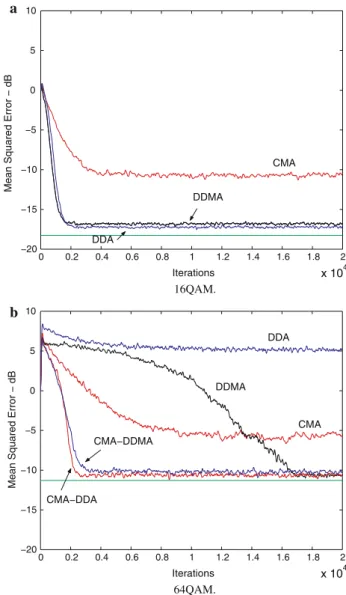
Figure3a shows the MSE for the DDA, DDMA and CMA with a 16QAM signal. It can be seen that the DDMA and the DDA have similar performances, with a steady-state error approximately 7 dB smaller than that provided by the CMA. In this case, it was not necessary to use the dual-mode algo-rithms. However, for a 64QAM signal, the dual-mode approach provides very good improvements, as shown in Fig.3b. For the single-mode algorithms, it may be remarked that the MSE performance of the DDMA is affected by the initial incorrect decisions. Even so, the DDMA converged,
0 0.2 0.4 0.6 0.8 1 1.2 1.4 1.6 1.8 2
x 104 −20
−15 −10 −5 0 5 10
Iterations
Mean Squared Error − dB
CMA
DDMA
DDA
16QAM.
0 0.2 0.4 0.6 0.8 1 1.2 1.4 1.6 1.8 2
x 104 −20
−15 −10 −5 0 5 10
Iterations
Mean Squared Error − dB
DDA
DDMA
CMA
CMA−DDMA
CMA−DDA
64QAM. a
b
2000 4000 6000 8000 10000 12000 14000 −15
−10 −5
0 5
Iterations
Mean Squared Error − dB
CMA−DDA SN=200
CMA−DDA SN=100 CMA−DDA
SN=400
CMA−DDMA SN=100
CMA−DDMA SN=200
CMA−DDMA SN=400 CMA−DDMA
SN=800 CMA−DDA
SN=800
MSE.
0 5 10 15 20 25 30
10−3 10−2 10−1 100
Symbol Error Rate (SER)
SNR (dB) CMA−DDMA, SN=800
CMA−DDA, SN=800 CMA−DDMA, SN=400 CMA−DDA, SN=400 CMA−DDMA, SN=200 CMA−DDA, SN=200 CMA−DDMA, SN=100 CMA−DDA, SN=100
CMA−DDA SN=100
CMA−DDA SN=200 CMA−DDA SN=400
SER. a
b
Fig. 4 MSE and SER for the CMA–DDMA and CMA–DDA for dif-ferent switching numbers
while the DDA did not, which confirms the better robust-ness of the DDMA in relation to the DDA. In addition, the DDMA and the DDA have a similar performance in a dual-mode approach.
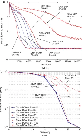
The main advantage of the CMA–DDMA over the CMA– DDA is the robustness to ISI provided by the DDMA, due to its greater robustness to phase-shifts and to the smaller number of “decision regions” of the DDM cost function in relation to the DD cost function. To illustrate this aspect, Fig.4a shows the MSE for these two techniques using a sec-ond simulation scenario. The algorithms were applied to the SPIB microwave channel # 2 (see http://spib.rice.edu/spib/ microwave.html) sampled at the baud rate, with 64QAM sig-nals, a SNR of 30 dB and an equalizer with 20 taps. In this case, the dual-mode approach is used with a hard switching introduced by a SN. Four different values of SN were con-sidered. We can note that when SN=100 and SN=200,
Table 4 SER and SAER provided by the CMA
Iterations 100 200 400 800
SER 0.613 0.574 0.485 0.334
SAER 0.527 0.494 0.418 0.289
the CMA–DDA does not perform so well, compared to the CMA–DDMA. This happens because when the switching is done, the level of ISI is not sufficiently low to switch to the DDA. In such a situation, the use of the CMA–DDA scheme will probably require the data retransmission, while the CMA–DDMA will probably not. Thus, the CMA–DDMA technique can significantly improve the system throughput. However, for SN=800, i.e. when the decision directed algo-rithms operate with a smaller level of initial ISI, the two algorithms provide roughly similar performances. This fact can be verified on the symbol error rate (SER) curves in Fig.4b. From this figure, we can conclude that the CMA– DDMA gives the same performances for the four values of SN, which is not the case for the CMA–DDA. The effect of the smaller number of “decision regions” of the DDM cost function in relation to the DDA cost function is pointed out in Table4, which shows the SER and the symbol amplitude error rate (SAER) for the CMA after 100, 200, 400 and 800 iterations. It can be concluded that the effective number of “decision errors” of the DDMA provided by the SAER is significantly smaller than that resulting from the SER for the DDA, specially for SN=100 and SN=200.
The theoretical relationship (25) between the approximate DDM (ADDM) and Wiener minima is illustrated by means of Table5 that shows the Wiener, DDM and ADDM min-ima. These simulation results were obtained in the noiseless case, with the channelh= [0.4 1]T, a two real-valued taps equalizer, a transmitted signal with a 4-PAM modulation and a transmission delay equal to 2. These results validate the approximation (25).
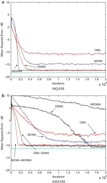
In what concerns the modified versions of the CMA and DDMA, in the case of the first simulation scenario with 16QAM signals, it can be seen from Fig.5a that the modified approach provides significant improvement (the MDDMA converges after 1,800 iterations and the DDMA after 4,500 iterations approximately). Again it was not necessary to use the dual-mode algorithms. Using 64QAM signals (Fig.5b), we remark that the DDMA has a faster convergence speed
Table 5 Wiener, DDM and ADDM minima
Wiener DDM ADDM
0 0.2 0.4 0.6 0.8 1 1.2 1.4 1.6 1.8 2
x 104 −20
−15 −10 −5 0 5 10
Iterations
Mean Squared Error − dB
CMA
MCMA
DDMA
MDDMA
16QAM.
0 0.2 0.4 0.6 0.8 1 1.2 1.4 1.6 1.8 2
x 104 −20
−15 −10 −5
0 5
10
Iterations
Mean Squared Error − dB
CMA MDDMA
MCMA
MCMA−MDDMA
CMA−DDMA DDMA
64QAM. a
b
Fig. 5 MSE for the CMA, MCMA, DDMA and MDDMA
than the MDDMA, which indicates that the MDDMA has a worst robustness to ISI than the DDMA. In a dual-mode version, the MDDMA outperforms all the other tested algo-rithms (MCMA–MDDMA converges after 1,500 iterations while CMA–DDMA needs 3,000 iterations for convergence, with the same steady-state error). It should be highlighted that all the DDM-based algorithms have steady-state errors close to the Wiener MSE.
7.2 RLS-type algorithms
Using the first simulation scenario of Sect.7.1, Fig.6a illus-trates the better performance of the RMDDMA (convergence after 350 iterations) and of the RDDMA (convergence after 550 iterations) in relation to the others. In this case, it was not necessary to use the dual-mode algorithms. The RLS–DD
0 1000 2000 3000 4000 5000 6000 7000 −20
−15 −10 −5
0 5
10
Iterations
Mean Squared Error − dB
RCMA RDDMA
RMCMA
RMDDMA
RLS−DD
16QAM.
0 1000 2000 3000 4000 5000 6000 7000 −20
−15 −10 −5 0 5 10
Iterations
Mean Squared Error − dB
RCMA RMCMA
RMCMA−−RMDDMA
RCMA−RDDMA
RMDDMA RDDMA
RLS−DD
64QAM.
a
b
Fig. 6 MSE for the RCMA, RMCMA, RDDMA and RMDDMA
algorithm corresponds to the RLS algorithm with the desired signald(n)replaced by the decided symbolaˆ(n).
In Fig. 6b, for 64QAM signals, it can be seen that the RMCMA has the better performance among the single-mode algorithms. Moreover, the dual-mode versions of the RDDMA and RMDDMA allow significant improvement of the convergence speed (RMCMA–RMDDMA converges after 700 iterations while the RCMA–RDDMA converges after 1,500 iterations approximately, with the same steady-state error.).
8 Conclusion
the decision device takes right decisions, it was proved that the DDMA has no local minima in the combined channel-equalizer impulse response space. In addition, in the case of real valued signals, an approximation of the DDM cost function has been derived in terms of the Wiener cost func-tion, valid in the neighborhood of the Wiener optimal solu-tion. Then, a relationship between the ADDM and Wiener solutions has been established, demonstrating the collinear-ity of these solutions. Simulation results have shown that the DDMA performs a good trade-off between the CMA and the DDA, in terms of robustness to initial ISI and performance. The DDMA has a better performance than the CMA, but a worst robustness with respect to the initial level of ISI. How-ever, it has a better robustness to initial ISI than the DDA. Furthermore, simulation results have shown that the CMA– DDMA equalization scheme provides a better robustness to ISI than the traditional CMA–DDA. A modified version of the DDMA, called the MDDMA, with its associated dual-mode version MCMA–MDDMA, have also been proposed. Finally, RLS-type versions of the previous algorithms have been derived to improve the convergence speed. Simulation results have illustrated the good trade-off between perfor-mance and robustness to the initial level of ISI, provided by the proposed algorithms, with the best performance being obtained with the RMCMA–RMDDMA.
Acknowledgments Carlos Alexandre R. Fernandes is scholarship sup-ported by CAPES/Brazil. The authors would like to express their thanks to Vicente Zarzoso for his useful comments.
Appendix A: Number of nonzero components
of a possible stationary point of the DDM cost function
In this appendix, it is demonstrated by contradiction that if a(n)has a uniform non constant modulus QAM distribution, then the solution (16) does not exist when NM ≥ 2. So, in the following developments, we assume thatNM ≥2.
We may rewrite the denominator of (16) as:D=(m4a+ 2σa4NM)(2σa4−m4a). As a uniform distribution has a neg-ative kurtosis, that ism4a −2σa4 < 0, D is positive. The numerator of (16), denoted byU, can be rewritten in the following way:
U =2σa8NM −m4a
m4a+2σa4(NM−1)
=2m4aσa4−m24a−2σ 4 aNM
m4a−σa4
, (A.1)
As we have:
Var|a|2=E
|a|2−σa2 2
=m4a−σa4>0, (A.2)
with E{|a(n)|4} =m4aand E{|a(n)|2} =σa2, we get:
m4a> σa4. (A.3)
From (A.1) and (A.3), it can be concluded that the maximum value ofUis obtained whenNMtakes its minimum value. As we have assumed NM ≥2, then NM =2 gives the highest value ofU, or equivalently:
U ≤ −m24a−2m4aσa4+4σa8. (A.4)
If we assume:
m4a> (
√
5−1)σa4, (A.5)
we get:
m4a+σa4 2
>5σa8⇒ −m24a−2m4aσa4+4σa8<0. (A.6)
The condition (A.5) is verified by the considered constel-lations, i.e. the circular non-constant modulus QAM con-stellations with uniform distribution. Consequently,U <0 and the solution (16) is negative, which is contradictory with |fτ|2≥0. So, we deduce thatNM =0 orNM =1.
Appendix B: The Hessian matrix of the DDM cost function
From (11) and (12) we have:
• fork=τ:
∂2JDDM ∂fk∂fk∗ =
4m4a|fk|2+4σa4
i=k
|fi|2−2σa4,
which gives:
∂2JDDM ∂fk∂fk∗
f=0
=−2σa4<0 and ∂ 2J
DDM ∂fk∂fk∗
f=eτ
=2σa4>0.
(B.1)
• For anyl,k=τ andk=l:
∂2JDDM ∂fl∂fk∗ =
4σa4fkfl∗,
which gives:
∂2JDDM ∂fl∂fk∗
f=0
=0 and ∂
2J DDM ∂fl∂fk∗
f=eτ
• For anyτ:
∂2JDDM ∂fτ∂fτ∗
=4m4a|fτ|2+4σa4
i=τ
|fi|2−2m4a,
which gives:
∂2JDDM ∂fτ∂fτ∗
f=0
=−2m4a<0 and
∂2JDDM ∂fτ∂fτ∗
f=eτ
=2m4a>0.
(B.3)
From the above calculations, we deduce the following expressions of the Hessian matrix of the DDM cost func-tion, at the stationary pointsf=0N+M−1andf=eτ:
∇2JDDM(f=0N+M−1)
=diag−2σa4, . . . ,−2σa4,−2m4a,−2σa4, . . . ,−2σa4
,
(B.4)
wherediag(·)is a diagonal matrix and the term −2m4a is the(τ, τ )t hentry of∇2J
DDM(f=0N+M−1), and:
∇2JDDM(f=eτ)
=diag2σa4, . . . ,2σa4,2m4a,2σa4, . . . ,2σa4
, (B.5)
where the term 2m4ais the(τ, τ )th entry of∇2JDDM(f=eτ).
Appendix C: Development of the RMCMA
Taking the gradient of the RMCMA cost function defined in Table3with respect tow, we get:
∇wφ (w)=4
n
i=0 λn−i
(yR2(i)−RR)yR(i)∂yR(i) ∂w∗
+(y2I(i)−RI)yI(i)∂yI(i) ∂w∗
, (C.1)
whereyR(i)andyI(i)denote, respectively, the real and imag-inary parts ofy(i), withy(i)=wTx(i). Equaling to zero this gradient at the pointw(n), we obtain:
n
i=0 λn−i
RRyR(i)+jRIyI(i)
x∗(i)
=
n
i=0 λn−i
yR3(i)+j yI3(i)
x∗(i). (C.2)
After some algebraic calculations, we get: n
i=0
λn−i[RRyR(i)+j RIyI(i)+ j yR(i)yI(i)y∗(i)]xH(i)
=w(n)T n
i=0
λn−i{|y(i)|2}x(i)xH(i). (C.3)
Let us define the quantitiesz(n)and(n)as:
z(n)= n
i=0 λn−i
RRyR(i)+ j RIyI(i)
+j yR(i)yI(i)y∗(i)
x∗(i), (C.4)
(n)= n
i=0
λn−is∗(i)sT(i), (C.5)
wheres(i)=y∗(i)x(i). Thus, equation (C.3) can be rewrit-ten as:
z(n)=(n)w(n), (C.6)
which leads to the following solution if(n)is nonsingular:
w(n)=(n)−1z(n). (C.7)
In the sequel, we develop a recursive form for (C.7). That needs to get recursions forz(n)and(n). However, these recursions cannot be found exactly becausez(n)and(n) depend onw(n), whilez(n−1)and(n−1)depend on w(n−1). So, we do the approximationw(n)∼=w(n−1), which is true in situations where the estimated vectorw(n) does not change quickly. Using this approximation, we obtain the following recursions forz(n)and(n):
z(n)=λz(n−1)+
RRyR(n)+ j RIyI(n)
+j yR(n)yI(n)y∗(n)
x∗(n), (C.8)
(n)=λ(n−1)+s∗(n)sT(n), (C.9)
By applying thematrix inversion lemma, a recursion for P(n)=(n)−1can be derived:
P(n)=λ−1
P(n−1)−k(n)sT(n)P(n−1), (C.10)
with
k(n)= P(n−1)s ∗(n)
λ+sT(n)P(n−1)s∗(n), (C.11) The gaink(n)can also be written as:
Using (C.8)–(C.11), we get from (C.7): w(n)=λP(n)z(n−1)+ [RRyR(n)
+j RIyI(n)+j yR(n)yI(n)y∗(n)]P(n)x∗(n), =P(n−1)z(n−1)−k(n)sT(n)P(n−1)z(n−1)
+[RRyR(n)+j RIyI(n)+j yR(n)yI(n)y∗(n)] ×k(n)/y(n),
=w(n−1)+k(n) 1
y(n){RRyR(n)+j RIyI(n)
+j yR(n)yI(n)y∗(n)−ξ(n)|y(n)|2}. (C.12) Expression (C.12) involves the a posteriori equalizer output y(n)=wT(n)x(n)and the a priori equalizer outputξ(n)= wT(n−1)x(n). But, at iterationn, we do not have access to the equalizer outputy(n), as it depends on the tap-weight vec-tor estimatew(n), not yet calculated. So, the outputy(n)in (C.12) is replaced by the a priori outputξ(n). This approx-imation is equivalent to the one done in (C.8) and (C.9). Then, taking this approximation into account, we may rewrite (C.12) as:
w(n)=w(n−1)+k(n) 1 ξ(n)
RRξR(n)+j RIξI(n)
+jξR(n)ξI(n)ξ∗(n)−ξ(n)|ξ(n)|2
, (C.13)
or
w(n)=w(n−1)+k(n) 1 ξ(n)
ξR(n)[RR−ξR2(n)]
+jξI(n)[RI−ξI2(n)]
. (C.14)
Thus, the RMCMA can be summarized by (C.10), (C.11) and (C.14), withs(n)replaced byξ∗(n)x(n).
References
1. Godard, D.N.: Self-recovering equalization and carrier tracking in two dimensional data communication systems. IEEE Trans. Com-mun.28(11), 1867–1875 (1980)
2. Treichler, J., Agee, B.: A new approach to multipath correction of constant modulus signals. IEEE Trans. Acoust Speech Signal Proces.31(2), 459–472 (1983)
3. Zeng, H.H., Tong, L., Johnson, C.R. Jr.: An analysis of con-stant modulus receivers. IEEE Trans. Signal Proces.47(11), 2990– 2999 (1999)
4. Schniter, P., Johnson, C.R. Jr.: Sufficient conditions for the local convergence of constant modulus algorithms. IEEE Trans. Signal Proces.48(10), 2785–2796 (2000)
5. Fijalkow, I., de Victoria, F.L., Johnson, C.R. Jr.: Adaptive fraction-ally spaced blind equalization. In: IEEE Digital Signal Process-ing Workshop, pp. 257–260 Yosemite National Park, 2–5 October (1994)
6. Touzni, A., Fijalkow, I., Treichler, J.R.: Fractionally-spaced CMA under channel noise. In: IEEE Int. Conf. on Acoustics, Speech and Signal Processing, vol. 5, pp. 2674–2677 Atlanta, 7–10 May (1996)
7. Larimore, M.G., Treichler, J.R.: Convergence behavior of the Con-stant Modulus Algorithm. In: IEEE Int. Conf. on Acoustics, Speech and Signal Processing, vol. 8, pp. 13–16 Boston (1983)
8. Brooks, D., Lambotharan, S., Chambers, J.: Optimum delay and mean square error using CMA. In: IEEE Int. Conf. on Acoustics, Speech and Signal Processing, vol. 9, pp. 3361–3364 Seattle, 12– 15 May (1998)
9. Ding, Z., Kennedy, R.A., Anderson, B.D.O., Johnson, C.R. Jr.: Ill-convergence of Godard blind equalizers in data communications systems. IEEE Trans. on Commun.39(9), 1313–1327 (1991) 10. Fijalkow, I., Manlove, C.E., Johnson, C.R. Jr.: Adaptive
fraction-ally spaced blind CMA equalization: Excess MSE. IEEE Trans. Signal Proces.46(1), 227–231 (1998)
11. Johnson, C.R. Jr., Schniter, P., Endres, T.J., Behm, J.D., Brown, D.R., Casas, R.A.: Blind equalization using the Constant Modulus criterion: a review. In: Proc. IEEE,86(10), 1927–1950 (1998) 12. Lucky, R.: Automatic equalization for digital communication. Bell
Systems Tech. J.44(4), 547–588 (1965)
13. Oh, K.N., Chin, Y.O.: Modified constant modulus algorithm: blind equalization and carrier phase recovery algorithm. In: Int. Conf. on Communications, vol. 1, pp. 498–502 Seattle, 18–22 June (1995) 14. Yang, J., Werner, J.-J., Dumont, G.A.: The multimodulus blind
equalization and its generalized algorithms. IEEE J. Selected Areas Commun.20(5), 997–1015 (2002)
15. Ready, M.J., Gooch, R.P.: Blind equalization based on radius directed adaptation. In: IEEE Int. Conf. on Acoustics, Speech and Signal Processing, vol. 3, pp. 1699–1702 Albuquerque, 3–6 April (1990)
16. Axford, R.A., Milstein, L., Zeidler, J.: A dual-mode algorithm for blind equalization of QAM signals: CADAMA. in Asilomar Con-ference on Signals, Systems and Computers, vol. 2, pp. 172–176 Pacific Grove, Sept. (1995)
17. Banovic, K., Abdel-Raheem, E., Khalid, M.A.S.: A novel radius-adjusted approach for blind adaptive equalization. IEEE Trans. Sig-nal Proces.13(1), 37–40 (2006)
18. He, L., Amin, M.G., Reed, C. Jr., Malkemes, R.C.: A hybrid adap-tive blind equalization algorithm for QAM signals in wireless communications. IEEE Trans. Signal Proces.52(7), 2058–2069 (2004)
19. Foschini, J.G.: Equalizing without altering or detecting data. AT & T Tech. J.64(8), 1885–1911 (1985)
20. Ding, Z., Johnson, C.R. Jr., Kennedy, R.A.: On the (non)existence of local equilibria of Godard blind equalizers. IEEE Trans. Signal Proces.40(10), 2425–2433 (1992)
21. Li, Y., Ding, Z.: Global convergence of fractionally spaced Godard (CMA) adaptive equalizers. IEEE Trans. Signal Pro-ces.44(4), 818–826 (1996)
22. Li, Y., Liu, K.J.R., Ding, Z.: Length- and cost-dependent local min-ima of unconstrained blind channel equalizers. IEEE Trans. Signal Proces.44(11), 2726–2735 (1996)
23. Fijalkow, I., Touzni, A., Treichler, J.R.: Fractionally spaced equal-ization using CMA: Robustness to channel noise and lack of dis-parity. IEEE Trans. Inf. Theory45(1), 56–66 (1997)
24. LeBlanc, J.P., Fijalkow, I., Johnson, C.R. Jr.: CMA fractionally spaced equalizers: Stationary points and stability under iid and temporally correlated sources. Int. J. Adap. Control Signal Pro-ces.12(2), 135–155 (1998)
25. Zeng, H.H., Tong, L., Johnson, C.R. Jr.: Behavior of fractionally-spaced constant modulus algorithm: mean square error, robustness and local minima. In: Asilomar Conf. on Signals, Systems and Computers, vol. 1, pp. 310–314 Pacific Grove, 3–6 Nov. (1996) 26. Enders, T.J., Anderson, B.D.O., Johnson, C.R. Jr., Green, M.: On
27. Enders, T.J., Anderson, B.D.O., Johnson, C.R. Jr., Green, M.: On the robustness of fractionally-spaced constant modulus criterion to channel order undermodeling: Part II. In: IEEE Int. Conf. on Acoustics, Speech and Signal Processing, pp. 3605–3608 Munich, 20–24 April (1997)
28. Sharma, V., Raj, V.N.: Convergence and performance analysis of Godard family of blind equalization algorithms. In: IEEE Int. Conf. on Communications vol. 4, pp. 2577–2582 11–15 May (2003)
29. Zeng, H.H., Tong, L., Johnson, C.R. Jr.: Relationships between the Constant Modulus and Wiener receivers. IEEE Trans. Inf. Theory44(4), 1523–1538 (1998)
30. Suyama, R., de F. Attux, R.R., Romano, J.M.T., Bellanger, M.: Relationship between constant modulus and Wiener criteria. In: GRETSI, Paris, France, 8–11 Sept. (2003)
31. Yuan, J.T., Tsai, K.D.: Analysis of the multimodulus blind equal-ization algorithm in QAM communication systems. IEEE Trans. Commun.53(9), 1427–1431 (2005)
32. Pickholtz, R., Elbarbary, K.: The recursive constant modulus algorithm: a new approach for real time array processing. In: Asilo-mar Conf. on Signals, Systems and Computers, vol. 1, pp. 627–632 Pacific Grove, 1–3 Nov. (1993)
![Fig. 1 Simplified structure of a communication system Channel + Equalizer v(n)a(n) x(n) y(n)h Dec[ • ] â(n)w](https://thumb-eu.123doks.com/thumbv2/123dok_br/15339180.558827/3.892.349.814.81.177/fig-simplified-structure-communication-channel-equalizer-dec-â.webp)