M1 and M2 indicators- new proposed measures for the
global accuracy of forecast intervals
Mihaela SIMIONESCU*, PhD
Romanian Academy, Institute for Economic Forecasting, Bucharest
Abstract
This is an original scientific paper that proposes the introduction in literature of two new accuracy indicators for assessing the global accuracy of the forecast intervals. Taking into account that there are not specific indicators for prediction intervals, point forecasts being associated to intervals, we consider an important step to propose those indicators whose function is only to identify the best method of constructing forecast intervals on a specific horizon. This research also proposes a new empirical method of building intervals for maximal appreciations of inflation rate made by SPF’s (Survey of Professional Forecasters) experts. This method proved to be better than those of the historical errors methods (those based on RMSE (root mean square error)) for the financial services providers on the horizon Q3:2012-Q2:2013 .
Keywords: forecast intervals, accuracy, historical errors method, RMSE, M1 indicator, M2 indicator
JEL Classification: E21, E27,C51, C53
1. Introduction
This research brings into attention to the researchers/academic environment some global accuracy indicators proposed by the author for the forecast intervals. Indeed, in literature there is not a specific measure of accuracy only for prediction intervals. The common solution is to consider the limits or the midpoints as point forecasts and then to compute the classical measures of accuracy.
The M1 and M2 indicator s proposed by the author have a single objective: to allow us to choose the best method of constructing forecast intervals. Obviously, a lower value for an M indicator compared to another one implies that the method corresponding to the first indicator generated better forecast intervals.
Another objective of this research is to proposed different versions of the historical errors method used in constructing the intervals. On the other hand, we proposed another empirical method of building prediction intervals by taking into account the specific evolution of the maximal forecasts offered by the SPF (Survey of Professional Forecasters). Moving average models are used to describe this evolution and the best forecast is built.
2. Literature
A retrospective presentation of the methods used to construct a confidence interval is done by Chatfield (1993). Williams and Goodman (1971) proposed the estimation of forecast intervals by using the historical forecast errors. The main hypothesis is that future prediction errors will have almost the same repartition as the historical forecast errors. A part of the data is used to construct the model and the errors are determined. Then, another observation is added up in the data set, increasing the sample utilized to determine forecast errors.
An empirical method was proposed by Gardner (1988), who used the forecasting model for entire set of data, computing within-sampleăpredictionăerrorsăată1,ă2,ă3,ă…k-steps-ahead from the time origins, and then calculating the variances of the errors for each of the lead times.
The model is not updated, and the different variances are computed using within-sample fitted errors. Confidence intervals use two main assumptions: errors normality and the standard deviation of the k-step-ahead errors. Makridakis and Winkler (1988) showed that actual forecast errors in average are too larger compared to in-sample fit errors. Therefore, Gardner (1988) used Chebychev inequality. This method gave good results compared to theoretical approaches of Bowerman and Koeler (1989) and Yar and Chatfield (1990). Taylor and Bunn (1999)
proposed a combination of theoretical and empirical approaches, the regression models fitting the empirical errors as a function of predicted lead time. The specification uses the theoretically derived prediction variance formulae.
Kjellberg and Villani (2010) presented the advantages and disadvantages of the interval based on models and of those built by the experts. Forecast methods based on models describe the complex relationships using endogenous variables, the transparency making easy the identification of mistakes that generated wrong predictions. The disadvantages are related to the difficulty of adapting the model to recent changes in the economy, as well as the too simple form of the models. Chatfield (1993) shows that forecast intervals are often too narrow not taking into account the uncertainty relatedătoămodelăspecification,ăproblemăthatăisăencounteredăalsoăinătheăexperts’ăassessment.ă
Christoffersen (1998) explains how to evaluate these intervals while the methods for measuring forecasts density are introduced later, being extended for bivariate data. There are proposed tests for forecasts intervals, then bayesian prediction intervals are built, that analyse the impact of estimator error on interval. Hansen (2005) built asymptotic forecasts intervals to include the uncertainty determined by the parameter estimator.
3. Methodology and results
Forecast intervals consider the assumption that the forecast error series is normally distributed of null average and standard deviation equals root mean square error (RMSE) corresponding to historical forecast errors. For a
probability of (1-α),ă forecast interval is calculated:
K
k
k
RMSE
z
k
X
k
RMSE
z
k
X
t(
)
(
),
t(
)
(
)),
1
,...,
(
/2
/2
.
)
k
(
X
t - punctual forecast for variableX
tk at time t2 /
z
- theăα/2ăquintileăofăstandardizedănormalădistribution.Fischer, Garcia-Barzana,ă Tillmannă șiă Winkeră (2012)ă assessedă theă predictions’ă accuracyă usingă theă forecastă intervals,ăusingătheăclassicalăaccuracyămeasuresăbyăcomparingătheăintervals’ăcentresăwithătheărealizations.ăăKnüppelă (2012) considered not only the case of middle points but also the limits in order to compute some accuracy measures.
We start from point forecasts that are represented in our case by the maximal appreciations of the financial services providers and by the non-financial services providers for the USA quarterly inflation rate. The source of data is the Survey of Professional Forecasters (SPF). The horizon of quarterly data series covers the period Q1:2003-Q2:2013. The real values are added to the set of predictions.
The methods for constructing the forecast intervals are:
Meth1- the method of historical errors when the deviation of the last quarter is used as accuracy indicator
Meth2- the method of historical errors when the root mean square error (RMSE) of the last 4 quarters is used as accuracy indicator
Meth3- the method of historical errors when the deviation of the last corresponding quarter is used as accuracy indicator
Meth4- the method of historical errors when the root mean square error (RMSE) of the entire previous period is used as accuracy indicator
Meth5- the predictions data series follows MA(1) processes, forecast intervals being constructing for the corresponding predictions
Table 1: Maximal appreciations for the USA inflation rate (%) and the registered values (%)
Quarter
Forecasts
of
the
financial
services
providers
Forecasts of the
non-financial
services
providers
The registered values
Q3:2012
3.7
4.4
2.1641
Q4:2012
3.4
3.42
2.1314
Q1:2013
2
4.1
2.1364
Q2:2013
2.2
2.7
2.0743
Source: Survey of Professional Forecasters (SPF)
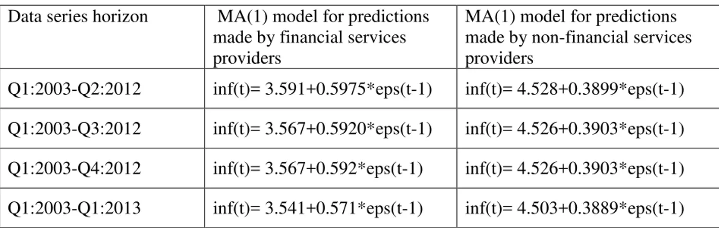
Theăinflationărateăatătimeă“t”ăisădenotedăbyăinf(t),ătheăerrorăbeingă“eps”.ăMA(1)ăprocessesăwereăbuiltăinăorderătoă describeătheăevolutionăofăSPF’săpredictions.ă
Table 2: MA(1) models for the predictions provided by the two types of services providers
Data series horizon
MA(1) model for predictions
made by financial services
providers
MA(1) model for predictions
made by non-financial services
providers
Q1:2003-Q2:2012
inf(t)= 3.591+0.5975*eps(t-1)
inf(t)= 4.528+0.3899*eps(t-1)
Q1:2003-Q3:2012
inf(t)= 3.567+0.5920*eps(t-1)
inf(t)= 4.526+0.3903*eps(t-1)
Q1:2003-Q4:2012
inf(t)= 3.567+0.592*eps(t-1)
inf(t)= 4.526+0.3903*eps(t-1)
Q1:2003-Q1:2013
inf(t)= 3.541+0.571*eps(t-1)
inf(t)= 4.503+0.3889*eps(t-1)
Source: own computations
Forăaămovingăaverageăprocessăinădescribingătheăevolutionăofăourăindicator,ătheăpredictionăatăaăfutureătimeă“n+h”ă has the following form:
=
∑
∑
- the coefficient
j- the index of time
The best forecast (f) is in this case:
∑
In our case, for one-step-ahead predictions, h equals 1 and the prediction is
.
The forecast error is given by:
∑
(
)
∑
In our particular case, the variance is:
Considering the hypothesis that the errors distribution is a normal one, the forecast interval is determined as:
√
. In our case, the forecast interval has the following form:, that
becomes
.
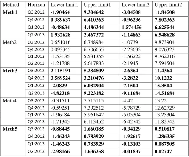
Table 3: Forecast intervals based on the mentioned methods
Method
Horizon Lower limit1 Upper limit1
Lower limit2 Upper limit2
Meth1
Q3:2012-1.90464
9.304642
-3.04508
11.84508
Q4:2012
0.389637
6.410363
-0.96236
7.802363
Q1:2013
-0.48634
4.486344
1.574456
6.625544
Q2:2013
1.932628
2.467372
-1.14863
6.548628
Meth2
Q3:20120.651016
6.748984
-1.0739
9.873904
Q4:2012
0.093345
6.706655
-2.23632
9.076323
Q1:2013
-1.53135
5.531355
-1.56222
9.762216
Q2:2013
-1.21788
5.617883
-2.1945
7.594504
Meth3
Q3:20122.115191
5.284809
-2.6364
11.4364
Q4:2012
3.589524
3.210476
-3.2832
10.1232
Q1:2013
-2.0829
6.082904
-7.1504
15.3504
Q2:2013
-4.82318
9.223182
-9.11684
14.51684
Meth4
Q3:2012-0.31511
7.715115
-4.42
13.22
Q4:2012
-0.59251
7.392512
-5.78729
12.62729
Q1:2013
-1.96184
5.961842
-5.05304
13.25304
Q2:2013
-1.71345
6.113452
-6.42742
11.82742
Meth5
Q3:2012-0.88445
1.660185
-0.34129
0.510817
Q4:2012
-1.46243
0.783929
-1.92617
1.286335
Q1:2013
-1.46243
0.783929
-0.13103
0.087505
Q2:2013
-2.98166
1.636258
-0.01837
0.02747
Source: own computations
M1 and M2 indicators allow us to make comparisons between methods or intervals according to the type of services providers.
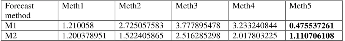
Table 4: M1 and M2 indicators for forecast intervals associated to financial services providers
Forecast
method
Meth1
Meth2
Meth3
Meth4
Meth5
M1
1.210058
2.725057583
3.777895478
3.233240844
0.475537261
M2
1.200378951
1.522405865
2.516285298
2.017803225
1.110706108
Source: own computations
A value closer to zero for each accuracy measure will indicate a better method for constructing the forecast interval and a better services provider. According to M1 and M2, the fifth method, proposed by the author according to the particular predictions, is the best for financial services providers.
Table 5: M1 and M2 indicators for forecast intervals associated to non-financial services providers
Forecast
method
Meth1
Meth2
Meth3
Meth4
Meth5
M1
1.618909142
1.84330988
3.819136806
3.565935309
0.808855517
M2
1.139244793
1.006849258
1.058443756
1.004606526
1.043421295
Source: own computations
According to M1 measure, the fifth method (meth5) proposed by me, gave the best results, for the financial services providers the forecast intervals being the best. The M2 indicator is a measure of the minimal deviations compared to the minimal deviations average (the weight of minimal deviations in the cumulated minimal deviations average for the two situations (when the real value is or not inside the interval)), the fifth method generating the best results for financial services financial, while the fourth method determined better intervals for non-financial providers. If M2 is decomposed on the two cases, we have to check which of the components has a higher value. It is preferred to have a small as possible weight of the errors outside the intervals. We have different results for the best provider according to M2. Therefore, we analyse the decomposition of the indicator on components and we chose the method for which the weight of errors for values outside the intervals is the lowest, in order to take the correct decision. In our case, all the values are inside the intervals; so, we take the decision according to M1 indicator. If we make a comparison with the accuracy of point forecasts, M1 measure corresponds to the measures based on errors’ăpercentage.
4. Conclusions
The main goal of this research was to introduce in literature a global accuracy measure specific to forecast intervals, taking into account that a particular accuracy indicator has not been proposed yet. Our M1 and M2 indicators were used in order to make comparisons between forecast intervals. For SPF maximal forecasts offered by financial and non-financial services providers our indicators put into evidence the superiority of our method for constructing intervals corresponding to financial institutions. On the other hand, the historical RMSE method gave the best results for non-financial agents if the longest historical horizon is taken into account.
Aălimitationăofătheăproposedăindicatorsăisătheăfactăthatăweăcan’tăassessătheăaccuracy/uncertainty by putting into evidence the specific sources of uncertainty. The interpretation should be done in a prudent way, because it does not have an economic significance. We use these measures only to fix the best method to construct the prediction intervals. We also checked the case when the centres of the intervals are considered instead of specific limits, but in this case lower values are obtained for all situations. Therefore, we concluded that M1 and M2 with higher values cover more sources of uncertainty.
References
[1] Bowerman,ă B.L.,ă andă Koehler,ă A.B.ă (1989),ă “Theă Appropriatenessă ofă Gardner’să Simpleă Approachă andă Chebychevă Predictionă Intervals.”ă published paper presented at the 9th International
[2] Chatfield C. (1993), Calculating interval forecasts, Journal of Business and Economic Statistics 11: 121-144. [3] Christoffersen, P. F. (1998), Evaluating interval forecasts, International Economic Review 39, p. 841-862
[4] FischerăH.,ăăGarcía-BárzanaăM.ă,ăăTillmannăP.,ăăWinkerăP.ă(ă2012),ă"EvaluatingăFOMCăforecastăranges:ăan interval data approach," MAGKS Papers on Economics 201213, Philipps-Universitätă Marburg,ă Facultyă ofă Businessă Administrationă andă Economics,ă Departmentă ofă Economicsă (Volkswirtschaftliche Abteilung)
[5] Gardner,ăE.ăS.,ăJr.ă“AăSimpleăMethodăofăComputingăPrediction Intervals for Time-Series Forecasts.”ăManagementăScience,ă34(1988):541-546. [6] Hansen B. (2005), Interval Forecasts and Parameter Uncertainty, Journal of Econometrics 135: 377-398.
[7] KjellbergăD.ăandăVillaniăM.ă(2010),ăTheăRiksbank’săcommunicationăofămacroeconomic uncertainty, Economic Review 1(2010): 2-49.
[8] KnüppelăM.ă(2012),ăIntervalăforecastăcomparison,ăInternationalăInstituteăofăForecastersă,ăTheăAnnualăInternationalăSymposiumăon Forecasting 24 - 27 June 2012, Boston, USA
[9] Makridakis, S., and R.L. Winkler, (1988),ă“SamplingăDistributionsăofăPost-SampleăForecastingăErrors.”,ăAppliedăStatistics,ă38,ă2(1988):ă331 -342.
[10] Taylor,ăJ.W.,ăandăD.W.ăBunnă(1999),ă“InvestigatingăImprovementsăinătheăAccuracyăofăPredictionăIntervalsăforăCombinationsăofăForecasts: A SimulationăStudy.”ăInternationalăJournalăof Forecasting, 15(1999):325-339.
[11] Williams,ăW.H.,ăandăGoodman,ăM.L.,ă(1971),ă“AăSimpleăMethodăforătheăConstructionăofăEmpirical,ăConfidenceăLimitsăforăEconomicForecasts.”ă Journal of the American Statistical Association, 66(1971):752-754.