Abstract—This research presents an associative classification with dissimilar rules (ACDR) algorithm to discover association rules with the highest priority and the top frequency. The proposed algorithm has the abillity to reduce redundant rules and to sort rules in decreasing order by their priorities. The results are dissimilar rules that can be used to predict information in the future. This algorithm can be applied as an associative classification technique and then sorted the results by interestingness measures. We develop the program with Rstudio, which is a very popular software package in statistical analysis and data mining. In the experimentation, we used the post-operative patients dataset to evaluate efficiency of the algorithm. The results confirm effectiveness of the ACDR algorithm by discovering a minimal but powerful set of association rules.
Index Terms—R Language, Association Rule, Algorithm Apriori, Associative Classification
I. INTRODUCTION
ssociation rule mining is to find the relations among data items from large database. The results can be used to predict future information or explain current relation. Apriori algorithm [1] is a popular method for association rule mining. This algorithm was developed based on AIS algorithm and focused on the pruning infrequent item sets. Many open-sources software can be used to discover the frequent patterns such as WEKA, which is software that can import data into the program and the final results are association rules, RapidMiner that has many tools for data mining and users can use operator chaining technique for mining with many algorithms in a single execution. But in this research we select the Rstudio for mining association rules because with this software, users can implement and extend algorithm easier than WEKA and RapidMiner that are Java implementation.
Rstudio is a suite of program environment to run the R language program, which is commonly language used to compute the statistics applications. This program environment provides several types of graphical display and has many libraries for discovering classification and association rules. In this research, we use the library arules because it can find the patterns with only a few lines of code. Moreover, this library was designed to allow users to Manuscript received November 30, 2012; revised January 10, 2013. This work was supported in part by grant from Suranaree University of Technology through the funding of Data Engineering Research Unit.
P. Kongchai is a doctoral student with the School of Computer Engineering, Suranaree University of Technology, Thailand, (email: [email protected]).
N. Kerdprasop is an associate professor with the School of Computer Engineering, Suranaree University of Technology, Thailand.
K. Kerdprasop is an associate professor with the School of Computer Engineering, Suranaree University of Technology, Thailand.
specify the mining for association rules with the constraints. With the constraint mining feature, it was thus easier and faster to find associative patterns with the proposed ACDR (Associative Classification with Dissimilar Rules) algorithm.
The main contribution of this research is proposing the ACDR algorithm. It can be used to discover dissimilar rules for classification. The algorithm has 5 main steps: searching for association rules, categorizing rules into target association rules and general association rules, classifying rules into groups by their right-hand-side item (RHS), analyzing with selected agent of each group, and sorting rules.
The proposed algorithm works with any dataset, but for the demonstration purpose, we apply the algorithm to the post-operative patients dataset.
II. RELATED WORK
This research aims to reduce the number of association rules that are redundant and retain the remaining rules that are important for predicting the future events. Kannan and Bhaskaran [4] proposed algorithm for reducing redundant rules by clustering association rules into many groups then cut redundant rules by interestingness measures. Mutter et al. [5] used CBA (Confidence-Based Association Rule Mining) algorithm to reduce the number of association rules. They ranked rules by confidence values then output rules for top hundred association patterns. Our work presented in this paper is different from others in that we used associative classification technique to rank and reduce association rules.
Associative classification technique is an integrated of classification rules and association rules. The goal of this technique is to search for the results having the format “If one item or more items have occurred, then another item must occur”. It is like the classification rules. Hranchotchuang et al. [3] used associative classification technique for predicting unknown class label by guessing the class label with association rules then the results will be classified with classification rules. Tang and Liao [7] proposed a new Class Based Associative Classification algorithm (CACA). Their algorithm tried to reduce the searching space and results are better accuracy of classification models.
Further this research also does the top ranking after the discovery of important association rules. The ranking technique is to sort rules in decreasing order by their priorities. There are many researches which focus on sorting rules [2], [6], [9], [10]. In this research, we use four criteria to rank priorities of the association rules. The four certeria are the size of the association rules, confidence, support and target rules.
Dissimilar Rule Mining and Ranking Technique
for Associative Classification
Phaichayon Kongchai*, Nittaya Kerdprasop, and Kittisak Kerdprasop
Algorithm ACDR
Input: Dataset D, Target items T. Output: Dissimilar Rules DR.
(1) Rrhs=1 = apriori(D) # Rrhs=1 = RHS equal 1 item (2) For each R ∈Rrhs=1 {
(3) If RHS == T { (4) G1 = group(R) (5) } else G2 = group(R) (6) }
(7) Rmerge = merge(RevDup(G1), RevDup(G2)) (8) MG = group_by_RHS(Rmerge)
(9) For each G ∈ MG { (10) agent = find_agent(G) (11) }
(12) DR = sort_by_4condition(agent) (13) return DR
III. METHODOLOGY
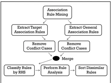
In this section we present ACDR algorithm for discovering association rules with the highest priority and the top frequency in descending order. The process of ACDR of two main parts, (1) to mine for association rules, and (2) to analyze association rules for finding important rules. We do the ranking priorities of the association rules with RStudio program. The details of ACDR algorithm, are shown in Fig. 1. Its diagrammatic flow is presented in Fig.2. Each subsection, A to E, is explanation of ACDR algorithm through the simple running example.
Fig. 1 ACDR (Associative Classification with Dissimilar Rules) algorithm.
Fig. 2 The process of ACDR algorithm.
A. Association Rules Mining
This research uses apriori algorithm [1] as a basis for further extension because its association rule mining steps are simple but highly efficient pruning strategy to remove infrequent item sets with minimum support measure (eq1). Support measure of item A is proportion of number of transactions that contain A to the total number of transactions in the database.
support(A) = |A|
|transactions| (1)
The results are frequent item sets 1Tthat can be used further1T
association rules constrained by the minimum confidence measure (eq2).
con�idence(A→B) = support(A∩B)
support(A) (2)
To implement the proposed methodology we are developed a program with R language which is suitable for data mining and the R system has many libraries for discovering association rules. For example to find association rules, the R code is as simple as the one show in Fig.3.
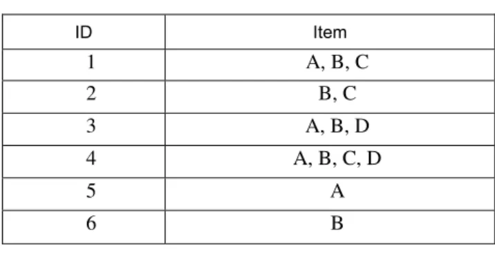
Fig. 3 The R code for association rule mining. From the commands in Fig.3 and the data as shown in Table 1, the result of program execution displayed in Table 2. With the simple six transactions given as the input, the output is a set of 17 association rules displayed in Table 2. These association rules have been constrained to contain exactly 1 item in the consequent part (or right-hand-side, RHS). This constraint is for later pruning the association rules.
B. Extract Target Association Rules and General Association Rules
This ACDR algorithm aims to predict or make decision on data that may occur in the future. Therefore, we applied a technique to include classification rules and association rules and call this technique is an associative classification. For our associative classification technique, we divided association rules into two groups, The first group is the rules to be defined by users contain target items (called Target Rules), and the second group is the rules not defined to contain target items (called General Rules). Target and general rule extraction is the step between lines 2-6 in Fig.1. Suppose the target item defined by users are item C and D, then the extracted target association rules are those illustrated in Table 3, whereas the rest (Table 4) is a set of general association rules.
library(arules) # call library arules
Tr <- read.transactions("test.txt",format="basket" ,sep=",")
# read file and storing data in format transaction. rules <- apriori(Tr, parameter= list(supp=0.1, conf=0.6, minlen = 2))
# association rule mining by apriori algorithm and set parameter with minimum support as 0.1, minimum confidence as 0.6 and the size of rules to contain at least 2 items.
TABLE1
EXAMPLE TRANSACTION DATABASE
ID
Item
1 A, B, C
2 B, C
3 A, B, D
4 A, B, C, D
5 A
6 B
TABLE2
ASSOCIATION RULES WITH A SINGLE ITEM IN THEIR RHS
NO.
Rules
Support
Confidence
1 {D} => {A} 0.333 1
2 {D} => {B} 0.333 1
3 {C} => {A} 0.333 0.667
4 {C} => {B} 0.5 1
5 {B} => {C} 0.5 0.6
6 {A} => {B} 0.5 0.75
7 {B} => {A} 0.5 0.6
8 {C,D} => {A} 0.167 1
9 {C,D} => {B} 0.167 1
10 {A,D} => {B} 0.333 1
11 {B,D} => {A} 0.333 1
12 {A,B} => {D} 0.333 0.667
13 {A,C} => {B} 0.333 1
14 {B,C} => {A} 0.333 0.667 15 {A,B} => {C} 0.333 0.667 16 {A,C,D} => {B} 0.167 1 17 {B,C,D} => {A} 0.167 1
TABLE3
TARGET ASSOCIATION RULES THAT CONTAIN
THE TARGET ITEMS C AND D IN THE RHS
NO.
Rules
Support
Confidence
5 {B} => {C} 0.5 0.6
12 {A,B} => {D} 0.333 0.667 15 {A,B} => {C} 0.333 0.667
The rules in Tables 3 and 4 may contain conflicting cases such as rule number 12 and 15 have exactly the same antecedent parts, but they predict different consequences. We call such case a conflict. At line 7 of the ACDR algorithm (Fig.1), we remove conflicting cases from both the target and general association rules. The remaining rules are shown in Tables 5 and 6.
TABLE4
GENERAL ASSOCIATION RULES
NO.
Rules
Support
Confidence
1 {D} => {A} 0.333 1 2 {D} => {B} 0.333 1 3 {C} => {A} 0.333 0.667
4 {C} => {B} 0.5 1
6 {A} => {B} 0.5 0.75
7 {B} => {A} 0.5 0.6
8 {C,D} => {A} 0.167 1
9 {C,D} => {B} 0.167 1
10 {A,D} => {B} 0.333 1
11 {B,D} => {A} 0.333 1
13 {A,C} => {B} 0.333 1
14 {B,C} => {A} 0.333 0.667 16 {A,C,D} => {B} 0.167 1 17 {B,C,D} => {A} 0.167 1
TABLE5
TARGET RULES AFTER REMOVING CONFLICT CASES
NO.
Rules
Support
Confidence
5
{B} => {C}
0.5
0.6
TABLE6
GENERAL RULES AFTER REMOVING CONFLICT CASES
NO.
Rules
Support
Confidence
6 {A} => {B} 0.5 0.75
7 {B} => {A} 0.5 0.6
10 {A,D} => {B} 0.333 1
11 {B,D} => {A} 0.333 1
13 {A,C} => {B} 0.333 1
14 {B,C} => {A} 0.333 0.667 16 {A,C,D} => {B} 0.167 1 17 {B,C,D} => {A} 0.167 1
C. Classify Rules by RHS (Right-Hand-Side) Item
The step at line 8 of the ACDR algorithm is to allocate rules into groups according to the items appeared in the RHS of the rules. The rule classifying strategy s as follow:
1. All items on the right hand side of association rules must be the same items. For example, from Table 6 rules 6, 10, 13 and 16 have the same item on their right hand side, which is B. Therefore, they are allocated as the same group.
2. Items on the right hand side are not the same, they will be allocated to the different groups.
TABLE7
GROUP C OF ASSOCIATION RULES
NO.
Rules
Support
Confidence
5
{B} => {C}
0.5
0.6
TABLE8
GROUP B OF ASSOCIATION RULES
NO.
Rules
Support
Confidence
6 {A} => {B} 0.5 0.75
10 {A,D} => {B} 0.333 1
13 {A,C} => {B} 0.333 1
16 {A,C,D} => {B} 0.167 1 TABLE9
GROUP A OF ASSOCIATION RULES
NO.
Rules
Support
Confidence
7 {B} => {A} 0.5 0.6
11 {B,D} => {A} 0.333 1
14 {B,C} => {A} 0.333 0.667 17 {B,C,D} => {A} 0.167 1
D. Rule Analysis
After classifying rules into groups, the next step is to select agent of each group (Fig. 1 line 9-11). These agents are for rule ranking and selecting. The criteria for rule selection are:
1. Select association rules with the longest size. The reason is that they can describe the complex conditions. For example, the patient who had a first degree of the tumor, had irradiated, had surgery and a healthy body then decision is that the patient is recovered from cancer.
2. Select association rules with the shortest size for describing the causes that may incur the damage. For Example, the patient who had the tumor and is in the final stage then the patient is cancerous.
From the rules in Tables 7-9, after analyzing rules with two criteria, we obtain the results as shown in Tables 10 and 11. Note that a single rule in group C remains the same one as shown in Table 7.
TABLE10
GROUP B AFTER RULE SELECTION
NO.
Rules
Support
Confidence
6
{A} => {B}
0.5
0.75
16
{A,C,D} => {B}
0.167
1
TABLE11
GROUP A AFTER RULE SELECTION
NO.
Rules
Support
Confidence
7
{B} => {A}
0.5
0.6
17
{B,C,D}
=> {A}
0.167
1
E. Sort Dissimilar Rules
The final process is to combine the three groups into one group and then sort the rules by the following criteria (Fig. 1 line 12).
1. If association rule was the shortest size, it will then be in the first order. If the rules are the same size, they will be considered by the next criterium.
2. If association rule is defined target item, it will be in the first order.
3. If association rule has the maximum confidence value, it will be in the first order. But if the rules have the same confidence value, they will be ranked by the next criterium.
4. If association rule has the maximum support value, it will be in the first order. But If the rules have the same support value, they will be ranked by order number.
The rules in Tables 7, 10 and 11 will be merged and then sorted with the four criteria. The results are shown in Table 12.
TABLE12
ASSOCIATION RULES AFTER SORTING
NO.
Rules
Support
Confidence
5 {B} => {C} 0.5 0.6
6 {A} => {B} 0.5 0.75
7 {B} => {A} 0.5 0.6
16 {A,C,D} => {B} 0.167 1 17 {B,C,D} => {A} 0.167 1
From Table 12 association rules NO. 5 contains defined items by user (item C and D), thus it is ranked first. Association rules NO. 6 and 7 are rules of the same size, they must be ranked by confidence value. Rule NO. 6 has higher confidence value than rule NO. 7, it is therefore ranked preceding rule No.7. Association rules NO. 16 and 17 are the same size and also the same confidence value and support value, they will be ranked according to the order number. The result is that NO. 16 has been ranked preceding rule NO. 17.
IV. EXPERIMENT
This research experimented with the post-operative patients dataset obtained from the UCI Machine Learning Repository [8]. The dataset has 8 attributes (explained in Table 13) and 90 transactions.
To perform the experiment, we developed a program using Rstudio environment and coding with R language for discovery association rules by apriori algorithm. We set minimum support and minimum confidence to be 0.01 and we define target items as ADM-DECS=I, ADM-DECS=S and ADM-DECS=A.
TABLE13
DESCRIPTION OF POST-OPERATIVE PATIENTS’ DATASET
Attribute Description
L-CORE patient's internal temperature in degree celsius:
high (> 37), mid (>= 36 and <= 37), low (< 36)
L-SURF patient's surface temperature in degree celsius :
high (> 36.5), mid (>= 36.5 and <= 35), low (< 35)
L-O2 oxygen saturation in %
excellent (>= 98), good (>= 90 and < 98), fair (>= 80 and < 90), poor (< 80)
L-BP last measurement of blood pressure high (> 130/90), mid (<= 130/90 and >= 90/70), low (< 90/70)
SURF-STBL
stability of patient's surface temperature : stable, mod-stable, unstable
CORE-STBL
stability of patient's core temperature : stable, mod-stable, unstable
BP-STBL patient's perceived comfort at discharge, measured as an integer between 0-10 and 11-20
ADM-DECS
discharge decision :
I (patient sent to Intensive Care Unit), S (patient prepared to go home), A (patient sent to general hospital floor)
TABLE14
THE PROCESS OF ACDR ALGORITHM AND NUMBER OF RULES AFTER
PERFORMING EACH PROCESS
Process
Number of rules (Rules)
1. Association Rule Mining 88,423 2. Extracting Target
Association Rules and General Association Rules
5,231
3. Classifying Rules by RHS items
5,231 4.Performing Rule
Analysis
1,048 5. Sorting Dissimilar rules 1,048
The results from Table 14 are important rules discovery with five sub-processes. The first sub-process is association rule with the consequent part containing 1 item and the result contains 88,423 rules. The second sub-process is to find target rules and general rules and also removing conflicting cases. The result contains 5,231 rules. The third sub-process is classifying rules by their RHS, the result is the same set of rules because this step classifies rules then inserts into group but does not remove any rules. The fourth sub-process is analyzing and selecting association rules by their sizes. The results are 1,048 rules. The last sub-process is sorting association rules, and the results are 1,048 rules.
Fig. 4 The results from ACDR algorithm.
The authors proposed an associative classification with dissimilar rules algorithm to discover association rules with the highest priority and the top frequency. The experimental results are composing of target rules and general rules. Target rules are the rules number 1-76 and general rules are the rules number 77-1,048. The rule number 1 can be interpreted as “if last measurement of blood pressure is low then discharge decision is to send the patient to general hospital floor”. The 1Tsymbol “?” in rule number 5 1Tmeans that
the attribute comfort has some effect to the decision ADM-DECS=I but we do not know the value.
V. CONCLUSION
This research introduces a design approach called ACDR (Associative Classification with Dissimilar Rules) to reduce redundant target and general association rules, then the results can be used to predict information as most classification rules. The ACDR algorithm consists of 5 main steps which are (1) finding association rules, (2) clustering target association rules and general association rules into two groups then removing redundant rules, (3) classifying rules into groups by their RHS item, (4) performing rule analysis with selected agent of each group, and (5) sorting rules according to proposed criteria. The dataset for algorithm evaluation is the post-operative patients dataset. The final result after processing the dataset through the five main steps of the ACDR algorithm is a minimal rule set
1. {L-BP=low} => {ADM-DECS=A}
2. {CORE-STBL=mod-stable} => {ADM-DECS=A}
3. {BP-STBL=stable,CORE-STBL=unstable} => {ADM-DECS=S} 4. {BP-STBL=stable,L-CORE=high} => {ADM-DECS=S} 5. {COMFORT=?,L-CORE=low} => {ADM-DECS=I} 6. {BP-STBL=stable,COMFORT=?} => {ADM-DECS=I} 7. {COMFORT=?,L-O2=good} => {ADM-DECS=I} 8. {COMFORT=?,L-SURF=mid} => {ADM-DECS=I}
9. {COMFORT=[11 - 20],CORE-STBL=unstable} => {ADM-DECS=S} 10. {CORE-STBL=unstable,L-BP=high} => {ADM-DECS=S} 11. {CORE-STBL=unstable,L-O2=good} => {ADM-DECS=S} 12. {BP-STBL=stable,COMFORT=[0 - 10],CORE-STBL=stable,L-BP=mid,L- CORE=mid,L- O2=excellent,L-SURF=mid,SURF-STBL=unstable} => {ADM- DECS=A}
13. {BP-STBL=stable,COMFORT=[0 - 10],CORE-STBL=stable,L-BP=high,L- CORE=mid,L-O2=excellent,L-SURF=mid,SURF-STBL=stable} => {ADM- DECS=A}
14. {BP-STBL=mod-stable,COMFORT=[0 - 10],CORE-STBL=stable,L-BP=high,L- CORE=low,L-O2=excellent,L-SURF=mid,SURF-STBL=stable} => {ADM- DECS=A}
15. {BP-STBL=stable,COMFORT=[0 - 10],CORE-STBL=stable,L-BP=mid,L- CORE=low,L-O2=excellent,L-SURF=low,SURF-STBL=stable} => {ADM- DECS=A}
…
77. {BP-STBL=stable,COMFORT=[0 - 10],CORE-STBL=stable,L-BP=mid,L- O2=excellent,L-SURF=mid,SURF-STBL=unstable} => {L-CORE=mid} 78. {BP-STBL=stable,COMFORT=[0 - 10],CORE-STBL=stable,L-CORE=mid,L- O2=excellent,L-SURF=mid,SURF-STBL=unstable} => {L-BP=mid} 79. {BP-STBL=stable,COMFORT=[11 - 20],L-BP=mid,L-CORE=mid,L-O2=good,L- SURF=mid,SURF-STBL=unstable} => {CORE-STBL=stable}
containing 1,048 rules, which are significantly decreased from the original 88,423 rules.
REFERENCES
[1] R. Agrawal, R. Srikant, “Fast algorithms for mining association rules,” In Proceedings of the International Conference on Very Large Data Bases, 1994, pp. 487-499.
[2] S. Bouker, R. Saidi, S. B. Yahia, M. E. Nguifo. “Ranking and selecting association rules based on dominance relationship,” In Proceedings of the 24th IEEE International Conference on Tools with Artificial Intelligence, 2012.
[3] W. Hranchotchuang, T. Rakthanmanon, K. Waiyamai, “Using maximal frequent itemsets for improving associative classification,”
In Proceedings of the1st National Conference on Computing and Information Technology, 2005, pp 24–25.
[4] S. Kannan; R. Bhaskaran, “Association Rule Pruning based on interestingness measures with clustering,” IJCSI International Journal of Computer Science Issues, V.6, 2009, pp. 35-43.
[5] S. Mutter, M. Hall, E. Frank, “Using classification to evaluate the output of confidence-based association rule mining,” In Proceedings of Australian Conference on Artificial Intelligence, 2004, pp. 538-549.
[6] G. Peyman, M. R. Sepehri, B. Azade, F. Nezam, “Ranking discovered rules from data mining by MADM method,” Journal of Computing Issue 11. V.3. 2011, pp. 64.
[7] Z. Tang, Q. Liao, “A new class based associative classification algorithm,” IAENG International Journal of Applied Mathematics, 2007, Advance online publication.
[8] The UCI Repository Of Machine LearningDatabases and Domain Theories [Online]. Available: http://www.ics.uci.edu/~mlearn/ MLRepository.html
[9] R. Sá. De. C, C. Soares, M. A. Jorge, P. Azevedo, J. Costa, “Mining association rules for label ranking,” In Proceedings of the 15th Pacific-Asia conference on Advances in knowledge discovery and data mining, 2011, pp. 432-443.