abrupt transitions on a
1
/f
noise background
Martin Rypdal and Kristoffer Rypdal
Department of Mathematics and Statistics, University of Tromsø The Arctic University of Norway, Tromsø, Norway
Correspondence to:Martin Rypdal (martin.rypdal@uit.no)
Received: 27 October 2015 – Published in Earth Syst. Dynam. Discuss.: 9 November 2015 Revised: 7 March 2016 – Accepted: 14 March 2016 – Published: 31 March 2016
Abstract. In order to have a scaling description of the climate system that is not inherently non-stationary, the rapid shifts between stadials and interstadials during the last glaciation (the Dansgaard-Oeschger events) cannot be included in the scaling law. The same is true for the shifts between the glacial and interglacial states in the Quaternary climate. When these events are omitted from a scaling analysis the climate noise is consistent with a 1/f law on timescales from months to 105years. If the shift events are included, the effect is a break in the scaling with an apparent 1/fβlaw, withβ >1, for the low frequencies. No evidence of multifractal intermittency has been found in any of the temperature records investigated, and the events are not a natural consequence of multifractal scaling.
1 Introduction
The temporal variations in Earth’s surface temperature are well described asscalingon an extended range of timescales. In this parsimonious characterisation, a parameter β de-scribes how the fluctuation levels on the different timescales are related to each other. Theβ-parameter can be defined via the scaling of the spectral density function of the signal by the relation
S(f)= h|Te(f)|2i ∼f−β, (1)
whereTe(f) is the Fourier transform of the time recordT(t) andh. . .i denotes an ensemble average. An alternative is to measure the range of the variability on the longest timescales within a time window of length1tby
T1t(t)=
2 1t
t+X1t /2
i=t
T(t)− 2 1t
tX+1t
i=t+1t /2
T(t)
, (2)
and to define β via the following relation (Lovejoy and Schertzer, 2013):
h|T1t(t)|2i ∼1tβ−1. (3)
In this description, the temperature fluctuations would de-crease with scale ifβ <1, implying that the climate fluc-tuations become less prominent as we consider longer timescales, a picture which is somewhat different from the rich long-range variability indicated by proxy reconstruc-tions of past climate. On the other hand, a valueβ >0 would imply that variability increases with scale, a property that (if it were valid on a large range of timescales) would lead to levels of temperature variability inconsistent with reality. It is therefore a natural a priori working hypothesis that Earth’s typical temperature fluctuations, the climate noise, is charac-terised byβ≃1. Such a process is called a 1/f noise.
(ENSO), which places larger fluctuations on the times scales of a few years than what can be expected from a scaling model. Other examples are the Dansgaard–Oeschger (DO) cycles in the Greenland climate during the last glacial period, encompassing repeated and rapids shifts between a cold sta-dial state and a much warmer interstasta-dial state. The result of this phenomenon is that the glacial climate in Greenland has much larger millennial-scale fluctuations than what can be expected from a 1/f description. However, as we demon-strate in this paper, the temperature variations of both the stadial and interstadial climate states fit well with the 1/f -scaling, telling us that the deviation from 1/f scaling in the glacial climate arise from these regime shifting events. As we go to even longer timescales, we also observe anomalous fluctuation levels on timescales from 104 to 105 years that can be identified with the shifting between glacial and inter-glacial conditions.
One could argue that the DO cycles and the glaciation cy-cles are intrinsic to the climate system and should not be treated as special events, and their variations should be re-flected in a scaling description of the climate. This idea was forwarded by Lovejoy and Schertzer (1986), elaborated in many later papers, and expanded to timescales up to almost 1 Gyr in Lovejoy (2014). Here several scaling regimes are proposed, including a “break” in the scaling law with an ex-ponentβ≈1.8 on timescales longer than a century. A scal-ing model invokscal-ing two scalscal-ing regimes can account for the millennial-scale temperature fluctuations that are produced by the DO cycles, which are anomalous with respect to a 1/f model. However, the estimated scaling exponent will depend on the average “density” of DO events in the ice-core record used for the estimate, and since the events are not uniformly distributed over time, there is no uniquely defined scaling exponent for the last glacial period. Moreover, the scaling law would not be useful as a climate-noise model to use as a null hypothesis for determining the significance of particular trends and events, such as the anthropogenic warming over the last centuries.
The main message of this paper is that the 1/fnoise char-acterisation of the temporal fluctuations in global mean sur-face temperature is very robust. It is an accurate description for the Holocene climate, but it is also valid under both sta-dial and interstasta-dial conditions during glaciations, and during both glacial and interglacial conditions in the quaternary cli-mate. The 1/fcharacter of the climate noise provides us with robust estimates of future natural climate variability, even in the present state of global warming. Such an estimate would of course be invalidated by a future regime shift (a tipping point) to a warmer climate state provoked by anthropogenic forcing. A future observed change in the 1/f character of the noise could therefore be taken as an early warning signal for such a shift.
2 Data, methods and results
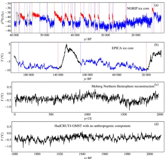
The analysis in this work is based on four data sets for tem-perature fluctuations: the HadCRUT4 monthly global mean surface temperature (Morice et al., 2012) in the period 1880– 2011 CE (Common Era), the Moberg Northern Hemisphere reconstruction for annual mean temperatures in the years 1– 1978 CE (Moberg et al., 2005), as well as temperature re-constructions from the North Greenland Ice Core Project (NGRIP) (Andersen et al., 2004) and the European Project for Ice Coring in Antarctica (EPICA) (Augustin et al., 2004). For the NGRIP ice core we have used 20-year means ofδ18O going back 60 kyr. For the EPICA ice core we have tempera-ture reconstructions going back over 300 kyr, but the data are sampled at uneven time intervals and the time between sub-sequent data points becomes very large as we go back more than 200 kyr. In addition we have used annual data for radia-tive forcing in the time period 1880–2011 CE (Hansen, 2005) to remove the anthropogenic component in HadCRUT4 data. Plots of all four data records are shown in Fig. 1.
2.1 Global versus local scaling
On the face of it, it is difficult to discern scaling laws for the climate noise on timescales longer than millennia, since we do not have high-resolution global (or hemispheric) tempera-ture reconstructions for time periods longer than two kyr. The ice core data available only allow us to reconstruct tempera-tures locally in Greenland and Antarctica, and we know from the instrumental record that local and regional continental temperatures scale differently from the global mean surface temperatures on timescales shorter than millennial. The dif-ferences we find are that local temperature scaling exponents βlare smaller than global temperature exponentsβg, and that
the ocean temperatures scale with higher exponents than land temperatures. Since there are strong spatial correlations in the climate system, it is possible that all local temperatures are scaling with a lower exponent than the global. In (Ryp-dal et al., 2015) this phenomenon is illustrated in an explicit stochastic spatio-temporal model. In this model, which is fit-ted to observational instrumental data, we find the relation-shipβg=2βl. This relationship is derived under the highly
inaccurate assumption that all local temperatures scale with the same exponent, but it is still a useful approximation in the following sections, where we will argue that we can use lo-cal and regional temperature records to discern the slo-caling of the global mean surface temperature on timescales of 10 kyr and longer. We do this by showing that the assumption that βg/βl>1 is valid on very long times scales leads to the
im-possible result that the variance of global averages becomes larger than the mean variance of local averages. Thus we con-clude thatβlconverges toβgon a sufficiently long timescale,
and we estimate an upper limit for that timescale.
Let us denote byσgandσlthe standard deviations of the
respec-Figure 1.(a)Theδ18O concentration in the NGRIP ice core dating back to 60 kyr before present (BP). Here present means AD 2000 (=2000 CE). The data are given as 20-year mean values. The time series are split into stadial (blue) and interstadial (red) periods.(b)The temperature reconstruction from the EPICA ice core. The shown time series are sampled with a time resolution of roughly 200 years. The temperature curve in the glacial periods is given in a blue colour.(c)The Moberg reconstruction for the mean surface temperature in the Northern Hemisphere. The data are given with annual resolution.(d)The HadCRUT4 monthly global mean surface temperature where the anthropogenic component has been removed using a linear-response model.
tively, on a monthly timescale. From Eq. (3) it follows that the ratio between the variances for the global and local tem-peratures at timescale1tis
ρ=(σg σl
)2(1t τ )
βg−βl,
whereτ =1 month. Unless we expect global temperatures to have larger variations than the local temperature at timescale 1t(the global temperature can not have a larger standard de-viation than the average standard dede-viation of the local tem-peratures), we must haveρ >1, or equivalently,
1t < τ(σl σg
)2/(βg−βl).
On the timescale of months, the fluctuation levels of local continental temperatures is about two orders of magnitude larger than the fluctuation level for the global mean temper-ature. If we also useβg=1 andβl=1/2 we obtain the
con-dition 1t <105 months∼10 kyr, i.e. on timescales longer
than 10 kyr the ratioβg/βlcan no longer be larger than unity.
A similar estimate can be obtained from the NGRIP ice core data. In the Holocene the 20-year resolution temperature re-constructions from Greenland has a standard deviation which is about five times greater than the 20-year moving average of the Moberg reconstruction for the Northern hemisphere. Applying the same argument restricts the timescale for which Greenland scaling exponent is smaller than the global scaling exponent to approximately 10 kyr.
Time scale
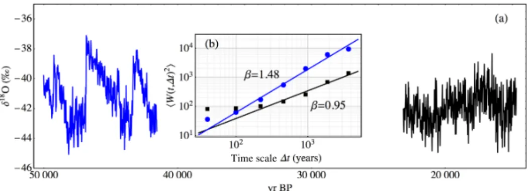
Figure 2.(a)Theδ18O concentration in the NGRIP ice core. The data are given as 20-year mean values. Two different parts of the times series are shown. The blue curve represents the δ18O concentration in a time period starting approximately 50 kyr before present (BP) and has a duration of approximately 8500 years. As in Fig. 1, present means AD 2000 (=2000 CE). The black curve represents theδ18O concentration in a long stadial period that started about 22 kyrs BP and has a duration of approximately 8500 years.(b)The wavelet scaling functions estimated from the two parts of the NGRIP data set. The blue points are the estimates from the part of the NGRIP ice core that is shown as a blue curve in(a), and which contains DO cycles. The black points are the estimates from the part of the NGRIP ice core that is shown as a black curve in(a), and which does not contain any DO cycles.
2.2 Methods for estimation of scaling
We use two methods to analyse the scaling of temperature records. The first is a simple periodogram estimation of the spectral power densityS(f). This estimator can also be ap-plied to data with uneven time sampling using the Lomb-Scargle method (Lomb, 1976). The other method is to take the wavelet transform of the temperature data:
W1t(t)= 1 √
1t
Z
T(t′)ψ(t−t
′
1t ) dt
′ (4)
and construct the mean square of the wavelet coefficients: the wavelet variance. This is a standard technique for estimating the scaling exponentβ(Malamud and Turcotte, 1999), and it is known that
h|W1t(t)|2i ∼1tβ. (5)
We choose to use the so-called Haar wavelet
ψ(t)=
1 t∈ [0,1/2) −1 t∈ [1/2,1)
0 otherwise
,
and the integral in Eq. (4) is computed as a sum. With this wavelet we have the relation
W1t(t)=T1t(t) √
1t , (6)
between the wavelet transform and the Haar fluctuation of Eq. (2). The power spectral density and the wavelet variance are equivalent representations of the second order statistics of the time record, one in frequency domain and the other in time domain, and Eqs. (1) and (5) show that they are characterised by the same exponentβ if there is scaling of the second moment. By the Wiener-Khinchin theorem, these
second-order moments are also equivalent to the autocorre-lation function. Hence, scaling in the second-order statistics plays a special role, irrespective of the scaling or non-scaling of other moments.
The wavelet variance method can be adapted to the case of unevenly sampled data using the method described in Love-joy (2014). In the present work, we obtain very similar re-sults using the periodogram and the wavelet variance estima-tors. Claims have been made that higher-order statistics in the form of a multifractal characterisation are an essential part of the statistical description of these data (e.g. Lovejoy and Schertzer (2013), Chapter 11). For this reason we include a brief analysis of higher moments of the data in Sect. 2.4, and discuss their significance in Sect. 2.5.
2.3 Results of second-order analysis
Time scale
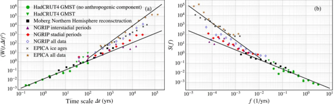
Figure 3.(a)For each time series considered in this paper we show double-logarithmic plots of the wavelet fluctuationh|W(t, 1t)|2ias a function of the timescale1t. The green triangles and the green circles represent the HadCRUT4 monthly global mean surface temperatures with and without the anthropogenic component respectively. The black circles are the analysis of the Moberg Northern Hemisphere recon-struction. The analysis of the 20-year mean NGRIP data is shown as the blue diamonds, the purple triangles and the red diamonds. The blue diamonds show the results of the analysis of the entire data set dating back to 60 kyrs BP. The red diamonds are the results of the analysis preformed on the stadial periods only, and the purple triangles are the results of the analysis of the interstadial periods only. The results for the EPICA ice core data are shown as the orange stars and the black crosses. The orange stars are obtained by analysis of the entire data set dating back 200 kyrs, and the black crosses are obtained by only analysing the two most recent glaciations. The two solid lines have slopes β=1 andβ=1.8.(b)As in(a), but instead of the wavelet fluctuation function we show the spectral density functionS(f). The two solid lines have slopes−βwithβ=1 andβ=1.8.
data (red diamonds) and the interstadial periods (purple tri-angles), which both display an approximate 1/f scaling, but where the fluctuation variance in the stadial data is larger than in the interstadial data. These results are different from what is obtained when considering the NGRIP data (during the last glaciation) as a single time series (shown as blue diamonds). If we were to define a single scaling exponent for the whole time series, then we would obtain an estimateβ≈1.4.
Figure 3 shows that the scaling of the stadial and intersta-dial NGRIP data are similar to the scaling of global temper-atures on shorter timescales during the Holocene. We have included an analysis of the instrumental temperature record both with (green triangles) and without the anthropogenic component (green disks). The anthropogenic component can be removed by subtracting the response to the anthropogenic forcing in a simple linear response model of the type consid-ered in Rypdal and Rypdal (2014). We have also included an analysis of the Moberg Northern Hemisphere reconstruction (black squares), and we observe that the composite scaling wavelet variance function and the composite spectral density function obtained by combining the instrumental data with the Moberg reconstruction, is consistent with a 1/f model on timescales from months to centuries. Since the NGRIP data also show 1/f scaling, and since we believe that the scaling of the NGRIP data is a reflection of global scaling on timescales longer than a millennium, it is illustrative to adjust the fluctuation levels of the NGRIP data so that its Holocene part has a standard deviation close to that of the standard deviation of the 20-year means of the Moberg re-construction in the same time period. This means that we use the adjusted NGRIP data as a proxy for global temperature
2.4 A note on multifractal processes
The exponentβis well-defined as long as the power spectral density functionS(f) is a power law inf, or equivalently if the wavelet varianceh|W(t, 1t)|2iis a power law in1t. As mentioned in Sect. 2.3, if well-defined, theβexponent is re-lated to the temporal correlations in the signal via simple for-mulas. In fact, for a (zero-mean) stationary processT(t) with −1< β <1 we havehT(t)T(t+1t)i ∼(β+1)β1tβ−1and for (a zero-mean) process with stationary increments and 1< β <3 we haveh1T(t)1T(t+1t)i ∼(β−1)(β−2)1tβ−3, where1T(t) is the increment process of T(t) (Rypdal and Rypdal, 2012). Thus, the results presented so far in this paper do not rely on any assumptions of self-similar or multifrac-tal scaling. It is only assumed that the second-order moments h|W(t, 1t)|2iare well approximated by power-laws over an extended range of timescales.
A more complete scaling analysis can be performed if one imposes the more restrictive assumption that the wavelet-based structure functions h|W(t, 1t)|qi are power-laws in 1t, not only forq=2, but for an interval ofq values. The time record can be classified as multifractal only if this is true. It is then possible to define a scaling functionη(q) via the relation
h|W1t(t)|qi ∼1tη(q). (7)
Lovejoy and Schertzer (2013) defines a scaling function ξ(1t) from the moment h|T1t(t)|qi. From Eq. (5) we ob-serve that their scaling function is related to ours byη(q)= ξ(q)+q/2.
By Eqs. (5) and (7) we observe that η(2)=β. IfT(t) is self-similar (or if T(t) is the increment process of a self-similar process in the caseβ <1) we haveη(q)=βq/2, but in general, the η(q) may be concave (it bends down). Pro-cesses that exhibit power-law structure functions and strictly concave scaling functions can be characterised as multifrac-tal intermittent. A monofracmultifrac-tal is a special case of the mul-tifractal class. For a monofractal (monoscaling) process, the scaling function is linear inq.
In Fig. 4 we present a crude multifractal analysis of the data sets considered in this paper usingqvalues in the range from 0.1 to 4. For the Holocene we find linear scaling func-tions for both the instrumental record and the Moberg North-ern Hemisphere reconstruction, and in the NGRIP data we find linear scaling functions for the stadial periods and the interstadial periods when these are analysed separately, al-though, as we have already seen, there is a deviation from the 1/f scaling in the stadial periods for timescales shorter than about 200 years. If the NGRIP record is analysed with both stadial and interstadial stages included, then it is not clear how to define the scaling function since the shifts between the two types of stages cause a “break” in the power-law scaling of the wavelet-based structure functions. If we de-fineη(q) using the timescales shorter than 2 kyr we obtain a linear scaling function corresponding toβ=1.14, and if we
use the timescales longer than 4 kyr we obtain a linear scaling function corresponding toβ=1.78. In neither case do we obtain a strictly concave scaling function. A linear scaling function is also obtained if we disregard the “break” in the scaling and fit power laws using all the available timescales. In this case the scaling function corresponds toβ=1.26. For the periods of the EPICA record that corresponds to ice ages, we find wavelet-based structure functions that are closer to power-laws than what is observed in the NGRIP record. This is expected since the abrupt transitions between cold and warm periods is much less pronounced in Antarctica than in Greenland. The scaling function for the ice-age periods in the EPICA data is linear and corresponds toβ=1.18.
The results discussed above show that from this analysis there is no evidence of multifractal intermittency in the tem-perature records analysed in this paper. This is not very sur-prising and could be suspected by direct inspection of the data record. The trained observer would use the fact that if η(q) is strictly concave, then the kurtosis ofW1t(t),
h|W1t(t)|4i h|W1t(t)|2i2∼
1tη(4)−2η(2),
is decreasing as a power-law function of1t, and is there-fore leptokurtic1on the shorter timescales1t. Multifractal intermittency in addition implies that the amplitudes of the random fluctuations are clustered in time, on all timescales, as observed in intermittent turbulence or financial time series (see e.g. Bouchaud and Muzy, 2003). These arenot promi-nent features in the time series analysed in this paper. For the NGRIP data, theδ18O ratio slightly deviates from a nor-mal distribution as a result of the DO events, but this is not well described by a multifractal model since that would re-quire the wavelet-based structure functions to be power-laws in1t. In fact, what we show in this paper is that the effect of DO events is to break the scaling, rather than to produce multifractal scaling.
Admittedly this multifractal analysis is a crude first-order characterisation. Our crude analysis suggests that the records analysed are most reasonably modelled as monofrac-tal. However, to establish this with confidence we need to perform statistical hypothesis testing. The strategy for such testing must consist of two elements. First, we have to test whether we can reject the hypothesis that the observed records are realisations of a multifractal (with monofractal as a special case) stochastic process. If this hypothesis can be rejected, there is no point in discussing whether the process is multifractal or monofractal. If we cannot reject the multi-fractal hypothesis, we must test if we can reject that this mul-tifractal is a monofractal. The outcome of these tests depends on the lengths of the observed records, since rejection of the various null hypotheses depends on the statistical uncertainty
1A distribution is leptokurtic if it has high kurtosis compared
Time scale Time scale
Time scale Time scale
Time scale Time scale
Figure 4.(a)The estimated wavelet-based structure functionsh|W(t, 1t)|qifor the HadCRUT4 monthly global mean surface tempera-ture where the anthropogenic component has been removed using a linear-response model. The lines show the fitted power-law functions cq1tτ(q). Theqvalues areq=0.1,1.0,1.5, . . .,4.0.(b)The scaling functionτ(q) obtained from the fitted power laws in(a). The line is a linear fit to the estimated scaling function, and the slope of this line isβ/2 withβ=0.88.(c–d)As(a)and(b)but in this case for the Moberg Northern Hemisphere reconstruction.(e–f)As(a)and(b)but for the interstadial periods in the NGRIP record.(g–h)As(a)and(b) but for the stadial periods in the NGRIP record.(i–j)As(a)and(b)but for the ice age periods in the EPICA record.(k–l)As(a)and(b)but for the NGRIP record including both stadial and interstadial periods. The red curve in(l)is the scaling function estimated from the longest timescales, the blue curve is the scaling function estimated from the shortest timescales, and the green curve is the scaling function estimated using all the available timescales.
associated with realisations of the null models. Monte Carlo simulations of these null models is the simplest tool to estab-lish these uncertainties. In a forthcoming paper we will per-form this rigorous testing of the multifractal hypothesis for the data analysed in the present paper, in addition to a wide selection of forcing data and climate model data. The results presented here should therefore be taken as preliminary.
2.5 A note on non-fractal processes that scale in the second moment
in the second moment, but not in other moments. Here we will not only demonstrate the existence of such processes, but explain that the serious fallacy of Lovejoy’s approach is that he fails to distinguish between multifractal noises and non-Gaussian noises that cannot be modelled within the mul-tiplicative cascade paradigm. Examples of the latter is the large class of Lévy noises. In less technical terms, the issue is that a multifractal noise may consist of uncorrelated random variables (e.g. their signs may be uncorrelated), but they will never be independent (e.g. their squares will be correlated). A Lévy noise, on the other hand, consists of independent ran-dom variables, which implies that all powers of the variables will be uncorrelated. Empirical multifractal analysis methods typically fail to distinguish between these different classes of processes because they implicitly assume a multifractal model. Often, the distinction is not easy to make, because a non-Gaussian Lévy noise may have a bursty (intermittent) appearance, and analysis must be designed to separate mul-tifractal clustering (correlation in higher powers) from inter-mittency of non-Gaussian independent variables. Long-range memory in the process does not make the distinction less rel-evant. Such processes may easily be produced from those discussed above by convolving the zero-memory processes with a memory response kernel.
From a physical viewpoint, it is very important to dis-tinguish between these two classes of stochastic processes. The multifractal processes are based on a turbulent cascade paradigm and the dynamical description is fundamentally nonlinear. The Lévy noises, and their long-memory cousins, may arise from non-Gaussian, independent fluctuations on the short timescales, e.g. jumps with randomly distributed waiting times.
We distinguish between a Lévy noise T(t) and a Lévy processX(t). The latter is a continuous-time stochastic pro-cess with stationary, identical and independently distributed (i.i.d.) increments, i.e. for any τ the incrementsX(t+τ)− X(t) have a well-defined distribution which is independent oft. The discrete-time processT(t)=X(t+1)−X(t), where t is the set of nonnegative integers, is a Lévy noise. Theoret-ical results on the fluctuation statistics on varying timescales of Lévy noises are most conveniently obtained by means of the standard structure functions of the underlying Lévy pro-cess (rather than the wavelet structure function defined in Sect. 2.4), i.e. we define
Sq(1t)≡ h|X(t+1t)−X(t)|qi.
For a process which belongs to the multifractal class we have
Sq(1t)∼1tζ(q),
where the scaling function ζ(q) is related to η(q) for the wavelet moments andξ(q) for the Haar fluctuation byζ(q)= η(q)+q/2=ξ(q)+q. In Appendix A we show that for a Lévy process the following relations hold for the second and
fourth moments;
S2(1t)= hY2i1t, (8)
S4(1t)=3hY2i2
1t2+
1
3kurt[Y] −1
1t
, (9)
where Y≡X(1) and kurt[Y] ≡ hY4i/hY2i2 is the kurtosis (flatness) of Y. For a Gaussian process kurt[Y] =3, and henceS4(1t)∝1t2. In this case Sq(1t)∝1tq/2, X(t) is a Wiener process, and T(t) is a Gaussian white noise. For a non-Gaussian Lévy noise, Eq. (9) provides the key to dis-tinguish it from multifractal noise. For1t∼kurt[Y]/3−1 there is a break in the scaling ofS4(1t). In fact, for1t≪
kurt[Y]/3−1 moments higher than q=2 will scale more or less like1t1(i.e.ζ(q)→1 for largeq), while for1t≫ kurt/3−1 they will scale like1tq/2. The latter corresponds to the scaling of a Gaussian white noise, which is quite ob-vious, since the random variables are independent and the central limit theorem implies that the fluctuations are Gaus-sian on the long timescales. On the other hand, on the short timescales when the fluctuations are still non-Gaussian, the scaling functionζ(q) bends over to become flat for largeq, which is just the behaviour we find for multifractals. Hence, by leaving out the scales1t >kurt[Y]/3−1 from the anal-ysis we will be led to the conclusion that the non-Gaussian Lévy process is multifractal. The trace-moment analysis em-ployed by Shaun Lovejoy (Schertzer and Lovejoy, 1987; Lovejoy and Schertzer, 2013) is designed to conceal the scal-ing behaviour on these scales and is not suitable as a model selection test to distinguish multifractals from non-Gaussian Lévy noises or their long-memory derivatives.
In Fig. 5 we present an analysis of a synthetic jump-diffusion process, which belongs to the class of Lévy noises. The details of this process are explained in Appendix B. The second-order structure function is a power law (a straight-line in the log-log plot), but the other structure functions are not. If a scaling function is produced by fitting a straight line to the structure functions on the long timescales, and comput-ing the slopes, we find the scalcomput-ing function of a white Gaus-sian noise (the red line in Fig. 5d). If the same is done on the short timescales, the estimated scaling function is con-cave as one would expect for a multifractal (the blue curve). In Fig. 6, we show the same for a jump-diffusion process with memory, produced by convolving the Lévy noise with a memory kernel. Hence, the difficulties related to distinguish-ing multifractals from other types of non-Gaussian processes are not something that is limited to processes of independent random variables.
3 Discussion and concluding remarks
Time scale
Figure 5.(a)The increments of a jump-diffusion process shown in(b). This is a non-Gaussian independent noise process.(b)A re-alisation of a jump-diffusion process, and the cumulative sum of the signal in(a). This process is the sum of a Brownian motion and a Poisson jump process as described in Appendix B. The jump distribution is Gaussian with a standard deviation that is 10 times greater than the standard deviation of the increments of the Brown-ian motion.(c)Sq(1tforq=1,2,3 for the jump-diffusion process as computed from a large ensemble of realisations of the process. (d) Scaling functionζ(q) estimated from structure functions like those in(c). The red line is estimated by computing the slope of the structure-function curves on the longest timescale (1t=500). The blue curve is estimated from the slopes at the shortest timescale ((1t=1). The black curve by estimating the slope of the straight line drawn between the end points of the structure-function curves.
change. For instance, when we apply standard statistical methods for estimating the significance of a temperature trend, the result depends crucially on the so-called error model, i.e. the model for the climate noise that is used as a null hypothesis. There is strong evidence that the tempera-ture fluctuations are better described by scaling models than by so-called red-noise models (or AR(1)-type models). How-ever, simply characterising the climate noise as scaling does not specify an error model. The exponent in the scaling law (theβ parameter) must also be determined, and it is usually determined from the same signal as we are testing for trends. If we do that without detrending we risk estimating a too high β for the error model, which yields a trend test with weak statistical power, i.e. we may fail to detect a trend even if it is present. It is possible to improve the statistical power in a logically consistent way by detrending prior to estimating β, but the approach is often (incorrectly) criticised for being circular, sinceβ should be estimated under the assumption
Time scale
Figure 6.As Fig. 5, but for a jump-diffusion process with memory as described in Appendix C. The parameter valueβ=0.4 is used.
that the error model (null hypothesis) is true. However, since de-trending only has a small effect if the null hypothesis is true, de-trending is valid under both the null hypothesis and the alternative hypothesis.
Another approach, which is the motivation for this paper, is to characterise the scaling of the climate noise from pre-industrial temperature records. If we are to use the scaling ex-ponent estimated from pre-industrial records to demonstrate the anomalous climate event associated anthropogenic influ-ence, we must be confident that the temperature scaling does not change significantly over time. We must also be confi-dent that the scaling is robust, in the sense that it is not too sensitive to moderate changes in the climate state. The re-sults presented in this paper suggest that, unless the climate system experiences dramatic regime shifting events, we can be confident that the natural fluctuations in global surface temperature is approximated by 1/f-type scaling on a large range of timescales. This result makes it easy to determine, on any timescale, if the observed increase in global mean sur-face temperature is inconsistent with the natural variability, and by how much.
assume thatX(1) belongs to the class of infinitely divisible random variables. This is a technical requirement that en-sures that an incrementX(t+1t)−X(t) has a well-defined distribution for arbitrary small1t. Since a Lévy process has stationary and independent increments, it is uniquely defined by the (infinitely divisible) distribution of X(1). In the fol-lowing we denoteY =X(1).
The characteristic function of the random variableY is de-fined as the φY(u)= heiuYi. If Y has a probability density functionpY, then
φY(u)=
Z
eiuypY(y) dy
is the Fourier transform ofpY. When working with Lévy pro-cesses it is common to define the functionψ(u) via the rela-tionφY(u)=eψ(u), andψ(u) is usually called the Lévy ex-ponent. Note that sinceφY(0)=1 we haveψ(0)=0. Since ψ(u) defines the random variableY it also determines the Lévy process uniquely. If t is an integer the value of X(t) is a random variable that can be written as a sum of lag-1 increments:
X(t)=(X(1)−X(0))+(X(2)−X(1))+. . .+(X(t)−X(t−1)).
This is a sum oftindependent copies of the random variable Y, and therefore the characteristic function ofX(t) is
φX(t)(u)= heiuYit=et ψ(u).
In general there is a simple relation between thenth moment of a random variable and thenth derivative of its characteris-tic function evaluated inu=0. Using this relation we can ex-press the moments ofX(t) via the formula (Gardiner, 2009),
hX(t)ni =i−n d n
dun|u=0e t ψ(u).
This implies that hX(t)i = −iψ′(0)t, so if we assume that the process does not have a linear drift, then we must have φ′(0)=0. The second moment is computed the same way:
hX(t)2i = − d
2
du2|u=0e
t ψ(u)
=t2et ψ(0)ψ′(0)2+t et ψ(0)ψ′′(0) = −ψ′′(0)t= hY2it.
Since increments are stationary we have the following result for the second order structure function:
S2(1t)=
D
|X(t+1t)−X(t)|2
E
= hX(1t)2i = hY2i1t.
= 1t e ψ(0) +61t e ψ(0) ψ (0)
+ 31t2e1t ψ(0)ψ′′(0)2
+ 41t2ψ(3)(0)e1t ψ(0)ψ′(0)+1t ψ(4)(0)e1t ψ(0) = 3ψ′′(0)21t2+ψ(4)(0)1t,
and sinceψ′′(0)= −hY2i andψ(4)(0)= hY4i −3hY2i2, we can write
S4(1t)=3hY2i21t2+(hY4i −3hY2i2)1t. (A1)
The ratio between the second and first terms in the above equation is
hY4i −3hY2i2 3hY2i21t =
kurt[Y] −3
31t ,
and hence we can conclude that S4(1t)∼1t2 for 1t≫
kurt[Y] −3 andS4(1t)∼1t for1t≪kurt[Y] −3.
Appendix B: A Poisson jump process
A Poisson jump process is defined via the Lévy exponent
ψ(u)=λ
Z
(eiux−1)dPJ(x),
wherePJ(x) is the distribution function for the jumps andλ is the rate for the occurrence of jumps. For simplicity we can imagine a process where we have positive jumps of fixed size x+:
dPJ(x)=δ(x−x+)
and
Hence the probability density function forX(t) becomes
pX(t)(x) =
1 2π
Z
e−iuxet ψ(u)du
= 1
2π
Z
e−iuxet λ(eiux+−1)du
= e
−λt
2π
Z
e−iuxet λeiux+du
= e
−λt
2π
Z
e−iux
∞
X
n=0
1 n!(t λe
iux+)ndu
= e
−λt
2π
∞
X
n=0
1 n!(λt)
n
Z
eiunx+e−iuxdu
= e−λt
∞
X
n=0
1 n!(λt)
n
δ(x−nx+)
There is a drift
hX(t)i =
Z
xPX(t)(x)dx=x+e−λt ∞
X
n=0
1 n!(λt)
nn =λt,
and
h|X(t)−λt|qi =
Z
|x−λt|qPX(t)(x)dx
=e−λt
∞
X
n=0
1 n!(λt)
n
|nx+−λt|q.
Appendix C: Lévy processes convolved with memory kernels
LetX(t) be a Lévy process and forβ∈(1,3), define a frac-tional Lévy process by
Z(t) =
0
Z
−∞
((t−s)β2−1−(−s)
β
2−1)dX(s)
+ t
Z
0
(t−s)β2−1dX(s)
= ∞
Z
−∞
((t−s)
β
2−1
+ −(−s)
β
2−1
+ ) dX(s)
= ∞
Z
−∞
Kβ(t, s)dX(s),
where
Kβ(t, s) = (t−s)
β
2−1
+ −(−s)
β
2−1
+ =(t−s)
β
2−12(t−s)
− (−s)β2−12(−s). Note that
Kβ(at, as) = (at−as)
β
2−12(at−as)−(−as)
β
2−12(−as)
= aβ2−1K(t, s),
and sincehdX(t)dX(s)i ∝δ(t−s)dt we have
hZ(t)2i = ∞ Z −∞ ∞ Z −∞
Kβ(t, s)Kβ(t, s′)E[dX(s)dX(s′)]
= ∞
Z
−∞
Kβ(t, s)2ds.
This implies that
hZ(at)2i = ∞
Z
−∞
Kβ(at, s)2ds
= ∞
Z
−∞
Kβ(at, as)2ads=aβ−1E[Z(t)2],
cher, H., Flückiger, J., Fritzsche, D., Fujii, Y., Goto-Azuma, K., Grønvold, K., Gundestrup, N. S., Hansson, M., Huber, C., Hvid-berg, C. S., Johnsen, S. J., Jonsell, U., Jouzel, J., Kipfstuhl, S., Landais, A., Leuenberger, M., Lorrain, R., Masson-Delmotte, V., Miller, H., Motoyama, H., Narita, H., Popp, T., Rasmussen, S. O., Raynaud, D., Röthlisberger, R., Ruth, U., Samyn, D., Schwander, J., Shoji, H., Siggard-Andersen, M. L., Steffensen, J. P., Stocker, T., Sveinbjörnsdottir, A. E., Svensson, A., Takata, M., Tison, J. L., Thorsteinsson, T., Watanabe, O., Wilhelms, F., and White, J. W. C.: High-resolution record of Northern Hemisphere climate extending into the last interglacial period, Nature, 431, 147–151, 2004.
Appelbaum, D.: Lévy processes – from probability to finance and quantum groups, Notices of the American Mathematica Society, 51, 1336–1347, 2004.
Augustin, L., Barbante, C., Barnes, P. R. F., Marc Barnola, J., Bigler, M., Castellano, E., Cattani, O., Chappellaz, J., Dahl-Jensen, D., Delmonte, B., Dreyfus, G., Durand, G., Falourd, S., Fischer, H., Flückiger, J., Hansson, M. E., Huybrechts, P., Jugie, G., Johnsen, S. J., Jouzel, J., Kaufmann, P., Kipfstuhl, J., Lam-bert, F., Lipenkov, V. Y., Littot, G. C., Longinelli, A., Lorrain, R., Maggi, V., Masson-Delmotte, V., Miller, H., Mulvaney, R., Oer-lemans, J., Oerter, H., Orombelli, G., Parrenin, F., Peel, D. A., Pe-tit, J.-R., Raynaud, D., Ritz, C., Ruth, U., Schwander, J., Siegen-thaler, U., Souchez, R., Stauffer, B., Peder Steffensen, J., Stenni, B., Stocker, T. F., Tabacco, I. E., Udisti, R., van de Wal, R. S. W., van den Broeke, M., Weiss, J., Wilhelms, F., Winther, J.-G., Wolff, E. W., and Zucchelli, M.: Eight glacial cycles from an Antarctic ice core, Nature, 429, 623–628, 2004.
Bouchaud, J.-P. and Muzy, J.-F.: Financial Time Series: From Batchelier’s Random Walks to Multifractal Cascades, in: The Kolmogorov Legacy in Physics, Lecture Notes in Physics, 636, 229–246, Springer-Verlag, Berlin Heidelberg, 2003.
Braun, H., Ditlevsen, P., Kurths, J., and Mudelsee, M.: A two?parameter stochastic process for Dans-gaard? Oeschger events, Paleoceanography, 26, PA3214, doi:10.1029/2011PA002140, 2005
Gardiner, C. W.: Stochastic Methods. A Handbook for the Natural and Social Sciences, Fourth Edition, Chapter 2, Springer, 2009. Hansen, J.: Earth’s Energy Imbalance: Confirmation and
Implica-tions, Science, 308, 1431–1435, 2005.
Lovejoy, S., Schertzer, D., and Varon, D.: Do GCMs predict the climate ... or macroweather?, Earth Syst. Dynam., 4, 439–454, doi:10.5194/esd-4-439-2013, 2013.
Malamud, B. D. and Turcotte, D. L.: Self-affine time series: I. Gen-eration and analyses, Adv. Geophys., 40, 1–90, 1999.
Moberg, A., Sonechkin, D. M., Holmgren, K., Datsenko, N. M., and Karlén, W.: Highly variable Northern Hemisphere temperatures reconstructed from low- and high-resolution proxy data, Nature, 433, 613–617, 2005.
Morice, C. P., Kennedy, J. J., Rayner, N. A., and Jones, P. D.: Quantifying uncertainties in global and regional tempera-ture change using an ensemble of observational estimates: The HadCRUT4 data set, J. Geophys. Res., 117, D08101, doi:10.1029/2011JD017187, 2012.
Rypdal, M.: Early-Warning Signals for the onsets of Greenland In-terstadials and the Younger Dryas-Preborial transition, J. Cli-mate, doi:10.1175/JCLI-D-15-0828.1, in press, 2016.
Rypdal, K., Rypdal, M., and Fredriksen, H.-B.: Spatiotemporal Long-Range Persistence in Earth’s Temperature Field: Analysis of Stochastic-Diffusive Energy Balance Models, J. Climate, 28, 8379–8395, 2015.
Rypdal, M. and Rypdal, K.: Is there long-range memory in solar ac-tivity on timescales shorter than the sunspot period?, J. Geophys. Res., 117, A04103, doi:10.1029/2011JA017283, 2012.
Rypdal, M. and Rypdal, K.: Long-Memory Effects in Linear Re-sponse Models of Earth’s Temperature and Implications for Fu-ture Global Warming, J. Climate, 27, 5240–5258, 2014. Schertzer, D. and Lovejoy, S.: Physical Modeling and Analysis
of Rain and Clouds by Anisotropic Scaling Multiplicative Pro-cesses, J. Geophys. Res, 92, 9693–9714,1987.
Svensson, A., Andersen, K. K., Bigler, M., Clausen, H. B., Dahl-Jensen, D., Davies, S. M., Johnsen, S. J., Muscheler, R., Parrenin, F., Rasmussen, S. O., Röthlisberger, R., Seierstad, I., Steffensen, J. P., and Vinther, B. M.: A 60 000 year Greenland stratigraphic ice core chronology, Clim. Past, 4, 47–57, doi:10.5194/cp-4-47-2008, 2008.