Repositório Institucional UFC: Dynamical universality of the contact process

PAPER

Dynamical universality of the contact process

To cite this article: L Böttcher et al 2018 J. Phys. A: Math. Theor.51 ₁₂₅₀₀₃

View the article online for updates and enhancements.

Related content

Ageing, dynamical scaling and its extensions in many-particle systems without detailedbalance

Malte Henkel

-Ageing in the critical contact process: a Monte Carlo study

José J Ramasco, Malte Henkel, Maria Augusta Santos et al.

-Ageing without detailed balance Tilman Enss, Malte Henkel, Alan Picone et al.

1

Dynamical universality of the contact

process

L Bö_ttcher1 _{, H J Herrmann}1,2 _{and M Henkel}1,3,4

1 _{ETH Zurich, Wolfgang-Pauli-Strasse 27, CH-8093 Zurich, Switzerland}

2 _{Departamento de Física, Universidade Federal do Ceará, 60451-970 Fortaleza,} Ceará, Brazil

3 _{Laboratoire de Physique et Chimie Théoriques (CNRS UMR 7019), Université} de Lorraine Nancy, BP 70239, F–54506 Vandœuvre-lès-Nancy Cedex, France 4 _{Centro de Física Teórica e Computacional, Universidade de Lisboa, P-1749-016} Lisboa, Portugal

E-mail: lucasb@ethz.ch

Received 18 December 2017, revised 2 February 2018 Accepted for publication 7 February 2018

Published 22 February 2018

Abstract

The dynamical relaxation and scaling properties of three different variants of the contact process in two spatial dimensions are analysed. Dynamical contact processes capture a variety of contagious processes such as the spreading of diseases or opinions. The universality of both local and global two-time correlators of the particle-density and the associated linear responses are tested through several scaling relations of the non-equilibrium exponents and the shape of the associated scaling functions. In addition, the dynamical scaling of two-time global correlators can be used as a tool to improve on the determination of the location of critical points.

Keywords: statistical physics, contact process, dynamical universality, ageing, scaling, correlators, response function

(Some figures may appear in colour only in the online journal)

1. Introduction

A great variety of dynamical processes in complex systems describe the spreading of innova-tions [1, 2], opinions [3–6], diseases [7–11], damage [12–14] or growing interfaces [15–20]. In recent years, considerable progress has been made towards a more profound understand-ing of spreadunderstand-ing dynamics and their correspondunderstand-ing phase transitions [7, 21–24]. The natural relation between phase transitions in statistical physics and those characterising spreading dynamics in complex systems allows to apply methods of statistical physics to classify spread-ing models based on their universal behaviour, i.e. the existence of the same characteristic

1751-8121/18/125003+16$33.00 © 2018 IOP Publishing Ltd Printed in the UK

asymptotic phenomena in different models and natural phenomena [21–23, 25–27]. More recently, advances in statistical physics suggested to study the so-called ageing phenomenon describing universal features of non-equilibrium relaxation properties between various mod-els [28]. A characteristic relaxation behaviour has, for example, been identified for the contact process (CP), a prominent example of the non-equilibrium directed percolation universality class [29–31], for stochastic Lotka–Volterra population dynamics [32, 33] or for gel-forming polymers [34].

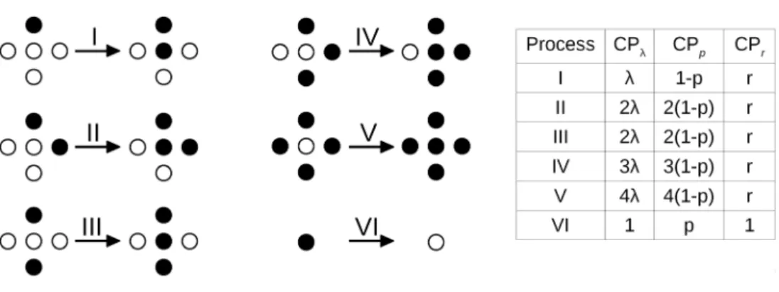
We shall study the relaxational properties of three different variants of the 2D CP which all have the same well-established stationary critical behaviour [13, 14, 22, 30]. Schematically, these variants are defined in figure 1, see section 2 for details. Starting from an initial state of uncorrelated particles with a given density, we are interested in the relaxation of both local and global two-time correlators of the particle-density, at the critical point, and also in the response of the particle-density to an external addition of particles5. The associated dynami-cal sdynami-caling is characterised by universal exponents and sdynami-caling functions which we can test. Until now, such tests of the scaling far from the stationary state were carried out in the 1D CP universality class [29–31, 35, 36], see also [37] for recent experimental data. Our findings on all three realisations of the 2D CP agree with (and extend) earlier results on local correlators [30] and also agree with experimental data of the turbulent liquid crystal MBBA [26, 38]. In particular, we shall explore to what extent the existing theoretical framework with its resulting scaling relations for the exponents [31] and predictions of the form of the scaling functions [18, 35, 39] can be tested. In addition, the two-time scaling of the global correlators can be used as a tool to improve estimates for the location of critical points. A better understanding of CP relaxation properties might be useful as benchmark to prepare the analysis of dynamical features for a variety of spreading dynamics such as disease or opinion spread and thus being of great importance for the design of appropriate control or intervention strategies.

This paper is organised as follows. In section 2 we describe the three variants of the CP in more detail and also introduce the necessary mathematical methods to analyse the scaling behaviour of the corresponding correlators and responses. All simulational results are pre-sented in section 3. In section 4 we derive the correlator and response function scaling forms. A summary of our results and our conclusions are given in section 5.

Figure 1. Update rules in 2D contact processes. Black sites are occupied and white sites are empty. The rates of the microscopic processes I–VI are given in the table, for the models CPλ, CPp and CPr. Throughout, spatial rotation-invariance of the reactions

is assumed.

5 _{For the contact process, the relaxation off the stationary critical point does not lead to dynamical scaling [29] and}

2. Model and methods

We study the relaxation characteristics of three models, defined on a square lattice, whose steady-state critical behaviour is identical to the one of the CP. Their steady-state universal-ity has been thoroughly checked numerically [12–14, 22]; here we shall consider the non-stationary critical behaviour and its universality. We refer to these models as CPλ, CPp and

CP_r. Based on a master equation, their update rules are formally specified in table 1 and are further illustrated in figure 1. While CPλ is the standard definition [22] of the contact process,

the variant CPp can be computationally more efficient and has been used previously to analyse the relaxation behaviour [30]. The model CP_p can be mapped onto CPλ by rescaling time

and setting p= (1+λ₎−1_{. Despite their similarity, we show in section 3.1 that the relaxation}

behaviour of CPλ and CPp is slightly different. For this reason, we consider both processes. The last model CP_r is a special case of a general threshold dynamics whose critical steady-state is known to fall into the CP universality class [13, 14]. In contrast to CPλ and CPp, the definition of CP_r does not distinguish between one or more occupied neighbours, see figure 1. If at least one neighbour is occupied, an empty nearest neighbour becomes occupied with a rate independent of the number of occupied neighbors. This is not the case for CPλ and CPp, where the occupation probability increases with the number of occupied neighbours.

Previous simulational studies on the CP relaxation characteristics have only been per-formed for the CPp model, in both 1D and 2D [30]. In 1D, the results agree with a transfer-matrix renormalisation group (TMRG) study [29] and a one-loop ε-expansion field-theoretic study [31] and in 2D, the Lotka–Volterra model falls into the same universality class [32]. It appears therefore timely to test thoroughly the universality of the non-equilibrium critical dynamics, by comparing simulational data with those of other variants of the contact process such as CPλ and CPr.

Non-stationary dynamics is achieved by starting from an initial state of uncorrelated parti-cles, with average density ni(0)=0.8. Then the control parameter is set to the critical value of the stationary state and the resulting dynamics is observed. Previous studies [29, 30, 32] have made it clear that in this setting, physical ageing arises, which is defined by the following properties [28]:

1. non-exponential, slow relaxation, 2. breaking of time-translation invariance, 3. dynamical scaling.

A process which satisfies only some, but not all, of these criteria may still undergo non-equilibrium dynamics, but does not display physical ageing, see e.g. [42] for a recent example. The existence of dynamical scaling in physical ageing implies that the underlying dynamics should exhibit universal dynamical features. These are measured through two-time autocor-relators and response functions. In order to study these quantities, we first define the average density

n(t):= 1

N

i

ni(t)=ni(t),

(1)

where we sum over all local densities ni(t)∈ {0, 1} representing empty or occupied lattice sites and N =L2

for a square lattice with linear dimension L. Spatial translation-invariance is assumed in equation (1) and throughout below. Next, we define the two-time local and global connected and unconnected autocorrelators, respectively, by [28] 6

C (2a)(t,s) =Clocal(t,s):=ni(t)ni(s) − ni(t)ni(s),

Γ(t,s) = Γlocal(t,s):=ni(t)ni(s),

(2b)

C (2c)(t,s) =Cglobal(t,s):=n(t)n(s) − n(t)n(s),

Γ(t,s) = Γglobal(t,s):=n(t)n(s).

(2d)

The first product in equations (2a) and (2b) runs over local densities with the same indices whereas the first product in equations (2c) and (2d) also takes cross terms into account, i.e. terms such as ni(t)nj(s) with i=j. The averaging procedure · denotes an ensemble average over time histories. Again, spatial translation-invariance is assumed. We denote the local cor-relators as C and Γ _{and the global ones as} C and Γ.

In terms of disease control, the correlators defined by equation (2) represent an important tool to quantify the prevalence of an epidemic after a certain time t as a consequence of an earlier infection at time s. As one example, the local unconnected correlator Γ(t,s) as defined by equation (2b) describes the probability of a disease to be locally found at time t after a local infection at time s. On the other hand, the local connected correlator C(t,s) defined by equation  (2a) is not taking into account the uncorrelated time evolutions n(t) and n(s). The global correlators C and Γ describe the disease correlations similarly to the local ones, however, considering the disease prevalence of the whole population. The quantities C/Γ and

C/Γ are an indication of the degree of correlation.

In ageing systems, one expects for these autocorrelators, with t,s≫τ_micro and t−s≫τ_micro

where τ_micro is a microscopic reference time scale, the following scaling behaviour [28]

C(t,s) =s−bfC(t/s) , fC(y)∼y−λC/z,

(3a)

Γ(t,s) =s−bf_Γ(t/s) , f_Γ(y)∼y−λΓ/z_,

(3b)

C (3c)(t,s) =s−bf_C(t/s) , f_C(y)∼y−λC/z_,

Γ(t,s) =s−bf_Γ(t/s) , f_Γ(y)∼y−λΓ/z_,

(3d) Table 1. Different contact process implementations on the square lattice.

Model I: CPλ [22] Model II: CPp [30] Model III: CPr [12–14]

1. Empty nearest neighbours of an occupied site become occupied at rate λ.

1. No dynamics occurs on empty sites. 1. Empty lattice sites, with at least one occupied neighbour, become occupied, at rate r.

2. Occupied sites become empty, at unit rate.

2. Occupied sites become empty with probability p. With probability 1−p, a new particle is created on an empty nearest-neighbour site.

2. Occupied sites become empty, at unit rate.

3. Gillespie’s algorithm is used to simulate the dynamics [40, 41].

3. One time-step corresponds to the inverse number of lattice sites.

where z is the dynamical exponent and the autocorrelation exponents λ_C,λ_Γ,λ C,λΓ

are defined from the asymptotics for y=t/s≫1 of the associated scaling func-tions. Occasionally, we also consider the complete time-space correlator defined by

C(t,s;r):=nr(t)n0(s) − n(t) n(s)=s−bFC

t s;

|r| s1/z

and its scaling behaviour. We shall

derive and test dynamical scaling relations between these exponents in section 3. Response functions can also be defined either locally or globally, according to [28]

R(t,s):= δni(t)

δhi(s)

hi=0

, R(t,s):= δn(t)

δh(s)

h=0

(4)

where hi(s) corresponds to the extra rate of a local creation of particles at site i and time

s and h(s) =N−1

ihi(s). While occasionally we shall consider the time-space response

R(t,s;r) = δ_δhnr₀₍(t_s)₎

hi=0

=s−1−aFR

t s;

|r| s1/z

, usually we shall just consider the autoresponse

R(t,s) =R(t,s;0_{). By analogy with the autocorrelators, one expects a dynamical scaling} behaviour of the response function [28]

R(t,s) =s−1−afR(t/s) , fR(y)∼y−λR/z,

(5a)

R(t,s) =s−1−af_R(t/s) , f_R(y)∼y−λR/z,

(5b)

along with the expected asymptotics of fR(y) and fR(y) for y=t/s≫1. As we shall show, the exponents of autocorrelators and autoresponses, defined in equations (3) and (5), are related by the following scaling relations

b=2δ _{, b=b}−d

z , a=a− d z

(6)

λ_Γ

z =

λ Γ

z =δ , λC=λC−d , λR=λR−d.

(7)

For relaxing systems with a non-equilibrium steady-state, starting from an initial non-vanish-ing particle density, the autocorrelation exponents are related to the stationary exponents as follows [31, 43–45]

λ_C

z =1+δ+ d z ,

λ C

z =1+δ.

(8)

Furthermore, the contact process has a specific symmetry, usually referred to as rapidity-reversal invariance. This leads to the further scaling relations [31]

b=1+a

(9a)

λ_C=λ_{R ,} λ C=λR.

(9b)

Numerical tests of these scaling relations will be presented in section 3, while their derivations will be given in section 4. To the best of our knowledge, previous studies solely focused on local correlators.

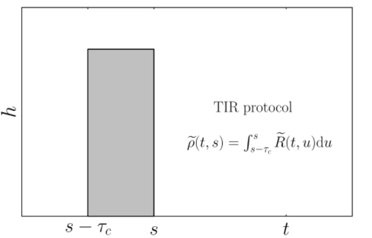
preferable to consider a spatially constant external field h, realised here as a particle addition rate, whose time-dependence is illustrated in the protocol shown in figure 2 [30]. Then one considers a kind of damage-spreading simulation, by computing

ρ(t,s) =

s

s−τc

duR(t,u) = lim

h→0

n(B)(t)−n(A)(t;s,τc)

h .

(10)

Herein, one compares two initially identical copies of the system which are updated by the same random numbers. At time s−τ_c copy A is exposed to a small field h>_{0 which is turned} off again at time s and the resulting particle-density n(A) _{is measured at time t. On the other} hand, copy B remains unperturbed, giving the particle-density n(B)_{. The perturbing field h is} applied on all sites, and the measured particle-densities are averaged over the whole lattice, such that cross-terms between different sites appear. Therefore, this integrated response ρ(t,s)

is indeed a global autoresponse, since

ρ(t,s) =

s

s−τc

du L−2d r,r′

R(t,u;r−_r′) = s

s−τc

duR0(t,u)≃τcR(t,s)

(11)

where Rk(t,s) is the Fourier transform of R(t,s;r), at momentum k and one assumes that

τ_c≪s is small enough.

3. Simulational results

We now describe the results of the numerical simulations of the non-stationary relaxation and ageing behaviour. Initially, the particles are uncorrelated and for the sake of comparabil-ity with the results of earlier studies we use an average denscomparabil-ity of ni(0)=0.8 [30]. Then the control parameter of the model (either λ_{, p, or r) is fixed, usually to its critical value (see}

equation  (12)), and we follow the system’s evolution. Unless stated otherwise, simulations have been performed on a square lattice with N =512×512 sites and periodic boundary conditions. In table 2 we collect our estimates for the exponents.

3.1. Particle density

At the critical point, the power-law behaviour n(t)=ni(t) ≃n∞t −δ

is expected, where δ_{=0.4505(10) denotes the decay critical exponent [46]. For the three realisations of the CP} under consideration, the critical points are [37, 40]







λ_{c=1.6488(1) ; CPλ}

pc= (1+λc)−1=0.377 53(2) ; CPp

rc=0.4724(1) ; CPr.

(12)

The value rc improves upon on the earlier estimate 0.47(1) [13] by a new method which is

described in the subsequent sub-section. In figure 3 we illustrate the relaxation of all three models towards their absorbing states. Clearly, all three models exhibit the same power-law relaxation behaviour. Thus, the dynamical exponent δ_{≃0.45 is found to be the same for all} three models, as expected from universality, and its value is in agreement with the literature.

3.2. Correlation functions

We now focus on the local and global correlators as defined by equation (2). First, in figure 4

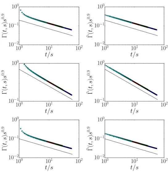
different variants of the contact process CPλ, CPp and CPr. Clearly, for all three realisations the expected scaling behaviour (3b) and (3d) is seen, where the value of the exponent b is consistent with the expectation b=2δ=0.901(2) [30]. For the local correlator, this is readily understood by re-writing the local unconnected correlator in terms of the connected one

Γ(t,s) =n(t)n(s)+C(t,s)≃s−2δ

n2∞

t

s

−δ

+f∞t s

−λ_C/z , (13)

where we used the late-time behaviour of the density n(t) ≃n∞t −δ

and the scaling form (3a) for the autocorrelator. Because of the known value δ=0.4505(10) [46] and the estimates λ_C/z=2.8(3) [30] or λ_C/z=2.58(2) [31], we have δ < λC/z such that the first term in equa-tion (13) dominates for large values of t/s. The slope of the plot is in agreement with the value λ_Γ/z=δ, expected from (7). An analogous, but slightly more involved argument applies to the global correlator Γ and will be presented in section 4.1 and confirms the measured value of b and of λ

Γ/z=δ≈0.45.

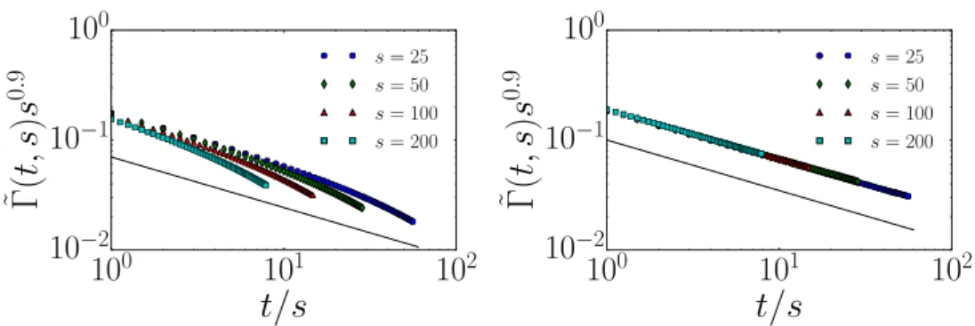
An application of the scaling of unconnected correlators concerns the refinement of esti-mates for the critical point. In figure 5 we consider the scaling of Γ in the CP_r model at the pre-vious estimate of rc≃0.471 [13]. The absence of a clear data collapse for r even slightly off

the precise value of rc is a result of the higher sensitivity of Γ with respect to small deviations

from rc as compared to the particle density n(t) since much larger time scales are explored.

Indeed, at the new estimate rc=0.4724(1) a perfect data collapse is observed as shown in

figure 5.

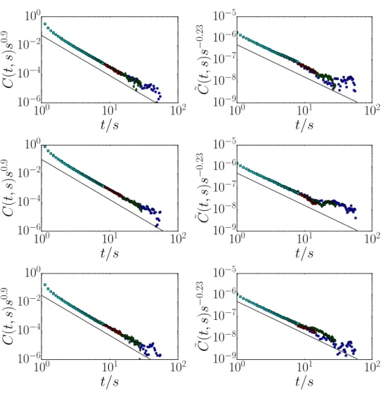
Next, in figure 6 we illustrate the scaling of the connected correlators C and C. The upper panel shows the local autocorrelators and their data collapse to produce the scaling form

C(t,s) =s−b_f C

t s

, as expected from equation  (3a). A clear scaling behaviour is seen for all three models CPλ, CPp and CPr. The extracted values of the exponents agree with equa-tions (6) and (8). Similarly, the lower panels display the global connected autocorrelator C. The anticipated scaling from (3c) is found to be satisfied in all three models and the exponents agree with the expected scaling relations equations (6) and (8). We also see that for larger val-ues of t/s, the numerical values of notably the global correlators become very small and thus sensitive to effects of purely stochastic noise in the data.

s

−

τ

s

t

h

ρ(t, s) =_ss

−τcR(t, u)du

Figure 2. Field perturbation protocol. The time-integrated response (TIR) protocol is used to determine ρ(t,s). A field perturbation h>0 is applied to the dynamics in the time interval [s−τ_c,s] (grey shaded area). The integrated response is measured

In particular, the numerical estimates of the exponent b≃ −0.23 agree with the scaling

relation b=b−_d/z=2δ−_d/z=−_{0.231(2) derived in section 4.1. Furthermore, the}

meas-ured values of the exponents λ_C/z and λ

C/z do reproduce the expectation from the scaling relations (8).

3.3. Response function

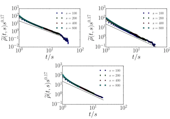
In figure 7 we illustrate the two-time scaling of the time-integrated global response ρ(t,s)

for the three variants of the contact process and different waiting times s. The scaling ansatz

ρ(t,s) =s−1−afρ(t/s) leads indeed to data collapses with 1+a=1+a−d/z=0.17(10), in agreement with the earlier findings in [30], but not with the scaling relation (9a), expected from field-theory [31]. On the other hand, from the asymptotic behaviour fρ(y)∼y−λR/z one

can extract the exponent value λ

R/z= (λR−d)/z=1.45(5) in good agreement with both the field-theoretic scaling relation (9b) [31], as well as with earlier simulations [30] and therefore also confirms the scaling relation (8).

It is surprising that the estimate a=0.3 is quite different from the field-theoretic expecta-tion a=−_{0.1, which means that the scaling relation} b=1+a expected from field-theory [31] is not confirmed by our numerical data for 2D, although the same numerical methods lead to data in agreement with that expectation for 1D dimensions [29, 30]. In order to test this fur-ther, we now consider the shape of the associated scaling function. This should allow to check against a simple oversight in the measurement of the global response ρ via equation (11) and

its interpretation through dynamical scaling.

Predictions on the shape of scaling functions beyond the context of a specific model can be obtained from generalisations of dynamical scaling. Indeed, in the context of the Table 2. Contact process dynamical critical exponents for 2D. The values of z and δ are taken from [23, table 4.3], and were used to compute the values of the non-equilibrium exponents from the scaling relations (6)–(9) [31], labelled ‘scaling’. The experimental data ‘exp’ are from the turbulent liquid crystal MBBA [38]. The numbers in brackets indicate the estimated uncertainty in the last given digit(s). For comparison, results of the earlier simulation [30] are also listed.

Exponent CPλ CPp CPr Exp Scaling

z 1.7660(16) 1.7660(16) 1.7660(16) 1.74(8) 1.7660(16)

δ 0.4505(10) 0.4505(10) 0.4505(10) 0.46(5) 0.4505(10)

λ_Γ/z 0.4505(10) 0.4505(10) 0.4505(10) 0.4505(10)

λ

Γ/z 0.4505(10) 0.4505(10) 0.4505(10) 0.4505(10)

λ_C/z 2.8(2) 2.8(2) 2.8(2) 2.5(3) 2.58(2)

2.8(3) [30]

λ

C/z 1.5(1) 1.5(1) 1.5(1) 1.4505(10)

b 0.901(2) 0.901(2) 0.901(2) 0.9(1) 0.901(2)

b −0.232(2) −0.232(2) −0.232(2) −0.232(2)

λ

R/z 1.45(5) 1.50(5) 1.45(5) 1.4505(10)

1.62(10) [30]

1+a 0.17(10) 0.17(10) 0.17(10) −0.232(2)

ageing behaviour of simple non-equilibrium magnets it has been proposed that the under-lying dynamical scaling can be extended to time-dependent conformal transformations, called local scale-invariance (lsi) [28, 48]. The autoresponse takes the explicit scaling form

ρ(t,s)∼R(t,s) =s−1−afρ(t/s), with the scaling function, for sufficiently large values of the scaling variable y=t/s, reads [39] (see section 4.2 for an outline of the derivation)

fρ,LSI(y) =fR,∞y1+a ′−λ_R/z

(y−₁)d/z−1−a′_.

(14)

Herein, the ageing exponent a=a+d/z and the new exponent a′ _{must be chosen for the}

optimal description of numerical data and fR,∞ is a normalisation constant7. As reviewed in

[28] and also verified for the 1D directed percolation universality class, the scaling function

fρ(y) to be read from equation (14) describes very well both simulational data [29, 35] as well as the one-loop expression derived from field-theory [31], provided the argument y2−_3.

We do not wish to discuss here whether the simple expression (14) can or cannot be consid-ered as an exact representation of the autoresponse scaling function but rather shall use it as a simple phenomenological tool to obtain in a different way an estimate for the ageing exponent

a, in the region of its approximate validity8_.

10

10

10

10

10

10

t

10

10

10

n

(

t

)

∼_t−_0.

45

λ= 1.6000

λ= 1.6488

λ= 1.6800

10

₁₀

₁₀

₁₀

₁₀

₁₀

₁₀

t

10

10

10

10

n

(

t

)

0.45

CPp CPλ

10

₁₀

₁₀

₁₀

₁₀

₁₀

t

10

10

10

n

(

t

)

∼_t−_0.

41 ∼_t−

0_.49

r= 0.450

r= 0.472

r= 0.500

Figure 3. Relaxation of the mean particle density. Upper left panel: for CPλ, the time

evolution of the density follows a power law with n(t)∼t−δ where δ=0.4505(10) [46]. Upper right panel: time evolution of n(t) for CPλ and CPp. Lower panel: time

evolution for CP_r. The critical points are given in equation (12). A square lattice with

N =1024×1024 sites was used. The black solid lines are guides to the eye with the specified slopes.

7 _{In mean-field descriptions of the ageing of simple magnets quenched to the critical temperature T=T}

c, or

generi-cally for quenches to T<_Tc in simple magnets, the scaling form (14) holds for the two-time autoresponse with

a=a′ _{[28]. The exact solution of the 1D Glauber}–_{Ising model, quenched to T=0 from a disordered initial state,}

produces a=0, a′₌₋1

2 [39].

8 _{For y}

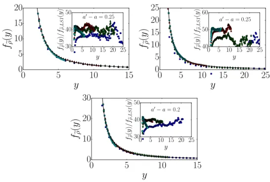
In figure 8 we show a comparison of our numerical data with the lsi-prediction (14). Indeed, for all three models the value a′ _{needed from equation (14) to describe the data is}

even larger than the value a≈0.3 read off from the simple collapse of the data. Observing that within the numerical accuracy a′−a≈0.2 for all three models gives a quantitative form of the expected universality of the scaling function and also illustrates that the value of a

needed to reproduce the shape of the scaling function appears to be even larger than the one deduced from achieving a data collapse. This comparison is further illustrated in the insets which display estimates for the ratio of scaling functions fρ(y)/fρ,lsi(y), for the values of

a′−a quoted in table 2. This shows to what extent the data collapse of dynamical scaling is actually achieved for finite values of s and the available statistics. The value a′−a≈0.2 is comparable to the estimate a′−a≈0.27 obtained (for non-logarithmic lsi) in the 1D contact

10

₁₀

₁₀

t/s

10

10

10

Γ(

t,

s

)

s

10

₁₀

₁₀

t/s

10

10

10

˜ Γ(

t,

s

)

s

10

10

10

t/s

10

10

Γ(

t,

s

)

s

10

10

10

t/s

10

10

˜ Γ(

t,

s

)

s

10

10

10

t/s

10

10

10

Γ(

t,

s

)

s

10

10

10

t/s

10

10

10

˜ Γ(

t,

s

)

s

Figure 4. Unconnected local and global correlators at the critical point. From top to bottom we show the data for CPλ, CPp and CPr. Left panels: Local unconnected

correlators Γ for different waiting times s. Right panels: Global unconnected correlators

process [39]. A more precise discussion of the shape of the scaling function near y≈1 does require high-quality data with large statistics and for very large waiting times s which at pre-sent are not available for the 2D contact process.

While these considerations give additional evidence for a value of the exponent a much larger than expected from the scaling relation (9a), and in agreement with earlier results [30], it remains an open problem why the computational technique based on equation (10) to find ρ

gives results in full agreement with field-theory in one spatial dimension and yet consistently produces a different result in two spatial dimensions.

4. Derivation of scaling forms

We present here the scaling arguments and establish the scaling relations as defined by equations (6)–(9).

4.1. Correlators

We begin with the unconnected correlators. In section 3.2, the local autocorrelator Γ(t,s) was already treated. Analogously, the global autocorrelator can be written as

Γ(t,s) =n(t)n(s)+C(t,s).

(15)

Comparing the data in figures 4 and 6, we see that the numerical values of the connected autocorrelator C(t,s) are much smaller than the values obtained for the unconnected autocor-relator, at least for the waiting times under consideration. Therefore, we arrive at the long-time scaling Γ( t,s) =s−2δ

n2∞(t/s) −δ

, in agreement with figure 4.

The smallness of C(t,s) can be understood from a specific symmetry of the directed per-colation universality class, which is known as rapidity-reversal invariance (rri). This sym-metry is the analogue of the time-reversal invariance of classical spin systems which relax to an equilibrium stationary state. For directed percolation, rri holds when the contribution of the initial state is suppressed in the field-theory action [31] and C(t,s)=0 only holds for an initial state distinct from the steady-state. On the other hand, since the long-time dynamics of

10

10

10

t/s

10

10

10

˜ Γ(

t,

s

)

s

0

.

9 s_s= 25_{= 50}

s= 100

s= 200

10

10

10

t/s

10

10

10

˜ Γ(

t,

s

)

s

0

.

9 s_s= 25_{= 50}

s= 100

s= 200

Figure 5. Unconnected global correlator dependence on deviations from the critical point. For the case of CP_r we show the sensitive dependence of the unconnected global correlator scaling on deviations from the critical point. Left panel: If one chooses

r=0.471<rc deviations from dynamical scaling can be seen. Right panel: if one sets

r=rc=0.4724, a clean data-collapse results. All data were averaged over more than

systems at the critical point of their steady-state is independent of their initial state, in critical directed percolation the influence of the initial state should disappear at long times such that

C(t,s)→0 very rapidly.

The discussion of the scaling of the global autocorrelator C(t,s) is based on the scaling assumption of the time-space correlator C(t,s;r), as follows

Figure 6. Connected local and global correlators at the critical point. From top to bottom we show the data for CPλ, CPp and CPr. Left panels: Local connected correlators

C(t,s) = 1 N2

i,j

(ni(t)− ni(t)) (nj(s)− nj(s))

= 1 N

i,j

(ni(t)− ni(t)) (n0(s)− n0(s))

≃

Rd

dr_C(t,s;r_{) =s}−b

Rd

dr_FC

t s;

|r_|

s1/z

=sd/z−b

Rd

du_FCt

s;|u|

(16)

where first spatial translation-invariance and then the scaling of the time-space correlator

C(t,s;r) was used. One thus finds b=b−d/z=−_0.231(₂)_.

The exponent λ_C/z has also been derived using a field-theoretical approach and found to fulfil the equality λ_C/z=1+δ+d

z [31].

4.2. Responses

Our discussion of the scaling of the response borrows from local scale-invariance [28, 48, 49]. A first consequence is that the full time-space scaling form factorises

R(t,s;r) =R(t,s)Φ

|r|(t−s)−1/z

, namely into the autoresponse R(t,s) and a universal

10

₁₀

₁₀

t/s

10

10

10

10

10

10

ρ

(

t,

s

)

s

s= 100 s= 200 s= 400 s= 800

10

₁₀

₁₀

t/s

10

10

10

10

10

ρ

(

t,

s

)

s

s= 100 s= 200 s= 400 s= 800

10

10

10

t/s

10

10

10

10

10

ρ

(

t,

s

)

s

s= 100 s= 200 s= 400 s= 800

Figure 7. Integrated response functions. Upper left panel: The integrated response of

CPλ. Upper right panel: The integrated response of CPp. Lower panel: The integrated

response of CP_r, for different waiting times s respectively. All data were averaged over more than 2·104 samples. The TIR protocol has been used with τ_c=25 and h=10−3.

scaling function Φ(u), which contains the space-dependence. With the normalisation Φ(0) =1, we obtain

ρ(t,s) =

s

s−τ_c

du R(t,u)(t−u)d/z

Rd

dqΦ(|q|)∼τcsd/z−1−a t

s

−(λ_R−d)/z

(17a) where we used the scaling form as defined by equation (5a) of the local autoresponse and only retained the leading asymptotics for y=t/s≫1. The temporal integral was estimated, for

s≫τ_c, from the mean-value theorem of integral calculus. Hence

ρ(t,s)∼s−(1+a−d/z)fρ(t/s) , fρ(y)∼y−(λR−d)/z.

(17b)

This scaling form of the global integrated response actually agrees with the one proposed in [31]. It also agrees with the scaling relations of equations (8) and (9b).

The shape of the scaling function fρ(y) is understood as follows. For the autoresponses, it is enough to concentrate on the lsi-transformation of the times. Indeed, under a change

t=β(t′_{) of the time coordinate, a quasi-primary scaling operator ϕ(t) of lsi transforms as}

follows [39]

0

5

10

15

y

0

5

10

15

20

f

(

y

)

0 5 10 15 20 25

y

30 40 50

fρ

(

y

)

/fρ,LS

I

(

y

)

a−a= 0.25

0

5

10

15

20

25

y

0

5

10

15

20

25

f

(

y

)

0 5 10 15 20 25

y

40 50 60

fρ

(

y

)

/fρ,LS

I

(

y

)

a−a= 0.25

0

5

10

15

y

0

10

20

30

f

(

y

)

0 5 10 15 20 25

y

30 40 50

fρ

( y ) /f ρ,LS I ( y )

a−a= 0.2

Figure 8. Scaling function of the global response. Upper left panel: The scaling function

fρ(t/s) of CPλ. Upper right panel: The scaling function fρ(t/s) of CPp. Lower panel:

The scaling function fρ(t/s) of CPr, for different waiting times s respectively. The

black solid lines represent the prediction (14) of lsi. The insets display the quotients

fρ(y)/fρ,lsi(y) =fρ(y)

y1+a′−λ_R/z_(y−1)d/z−₁−a′

, for the values of a′−a quoted in table 2. Waiting times: blue circles s=100, green diamonds s=200, red triangles

ϕ(t) =β˙(t′₎−x/z

t′dlnβ(t′)

dt′

−2ξ/z

ϕ′_(t′₎

(18)

where β(t) is an arbitrary, non-decreasing, differentiable function such that also β(0) =0 [39,

49]. According to Janssen-de Dominicis theory [27], a response function R(t,s) =ϕ(t)ϕ(s)

can be formally expressed as a correlator of the scaling operator ϕ associated to the order

param-eter (the particle-density for directed percolation) and the associated response scaling operator

ϕ. Because of equation (18), each scaling operator is characterised by two independent scaling

dimensions, which are denoted here by x=xϕ and ξ=ξϕ, or x=xϕ, ξ=ξϕ. If time-translations

were admitted (which would mean β(t) =β0 = 0 but this is excluded since β(0) =0) one would

have ξ=0 but ageing requires that time-translation-invariance should generically be broken. The requirement of covariance of the autoresponse function R(t,s) under these transformations and

(17a) readily produces equation (14), with a′−a=2

z

ξ+ξ [39, 49].

5. Discussion

Characterising phase transitions and universal features of spreading models have given invalu-able insights in different spreading dynamics [14, 21–23]. In our study, we focused on a clas-sification of the universality of dynamical properties of the contact process in two dimensions by considering three different numerical models. In addition to earlier studies, we also con-sidered the scaling of global correlators. Our results on the local correlators and the response function are in good agreement with earlier results [30, 32]. We derived an analytical relation between local and global correlators. All scaling exponents are summarised in table 2 and the expected universality between the three models considered in this work is clearly confirmed. All theoretically expected exponent scaling relations equations (6)–(9) were confirmed, with the only exception of (9a). A further analysis of the scaling function of the global response function revealed that this shape is numerically very well described by a simple version of local scale-invariance but also confirms the violation of (9a). This is surprising, since (9a) follows from standard field-theoretical arguments and the analogous numerical analysis in one spatial dimension is known to produce results consistent with (9a). We have shown that the scaling of the unconnected correlator is an appropriate tool to accurately determine critical points. Future studies might study the local integrated response to also test the scaling rela-tion as defined by equarela-tion (6). Such studies might also explore the relaxation dynamics in a parameter regime where the general contagion model CP_r allows for two coexisting stationary states in a cusp catastrophe phase space [13, 14].

Acknowledgments

We warmly thank José Javier Ramasco for helpful comments and suggestions. We acknowl-edge financial support from the ETH Risk Center and ERC Advanced grant number FP7-319968 FlowCCS of the European Research Council. We also thank the Instituto Nacional de Ciência e Tecnologia de Sistemas Complexos (INCT-SC) for financial support.

ORCID iDs

L Böttcher https://orcid.org/0000-0003-1700-1897

References

[1] Coleman J, Katz E and Menzel H 1957 Sociometry20 253

[2] Rogers E M 2010 Diffusion of Innovations (New York: Simon and Schuster) [3] Chwe M S 1999 Am. J. Sociol.105 128

[4] Leskovec J, Adamic L A and Huberman B A 2007 ACM Trans. Web15 [5] Böttcher L, Woolley-Meza O and Brockmann D 2017 PLoS One12 e0178062 [6] Böttcher L, Herrmann H J and Gersbach H 2018 PLoS One (in press)

[7] Pastor-Satorras R, Castellano C, Mieghem P V and Vespignani A 2015 Rev. Mod. Phys.87925 [8] Helbing D 2013 Nature497 51

[9] Böttcher L, Woolley-Meza O, Araújo N A M, Herrmann H J and Helbing D 2015 Sci. Rep.5 16571 [10] Böttcher L, Woolley-Meza O, Goles E, Helbing D and Herrmann H J 2016 Phys. Rev. E 93 042315 [11] Böttcher L, Andrade J S Jr and Herrmann H J 2017 Sci. Rep.7 14356

[12] Majdandzic A, Podobnik B, Buldyrev S V, Kenett D Y, Havlin S and Stanley H E 2014 Nat. Phys. 10 34

[13] Böttcher L, Luković M, Nagler J, Havlin S and Herrmann H J 2016 Sci. Rep.7 41729 [14] Böttcher L, Nagler J and Herrmann H J 2017 Phys. Rev. Lett.118 088301

[15] Henkel M, Noh J D and Pleimling M 2012 Phys. Rev. E 85 030102 [16] Halpin-Healy T and Takeuchi K 2015 J. Stat. Phys.160 794 [17] Henkel M and Durang X 2016 J. Stat. Mech.P07006

[18] Kelling J, Ódor G and Gemming S 2017 J. Phys. A: Math. Theor.50 12LT01 [19] Kelling J, Ódor G and Gemming S 2017 J. Phys. A: Math. Theor.51 035003 [20] Durang X and Henkel M 2017 J. Stat. Mech.P123206

[21] Grassberger P 1983 Math. Biosci.63 157

[22] Marro J and Dickman R 2005 Nonequilibrium Phase Transitions in Lattice Models (Cambridge: Cambridge University Press)

[23] Henkel  M, Hinrichsen  H and Lübeck  S 2008 Non-Equilibrium Phase Transitions Volume I: Absorbing Phase Transitions (New York: Springer)

[24] Gleeson J P 2013 Phys. Rev. X 3 021004 [25] Hinrichsen H 2000 Adv. Phys.49 815

[26] Takeuchi K A, Kuroda M, Chaté H and Sano M 2007 Phys. Rev. Lett.99 234503 [27] Täuber U C 2014 Critical Dynamics (Cambridge: Cambridge University Press)

[28] Henkel  M and Pleimling  M 2010 Non-Equilibrium Phase Transitions, Volume 2: Ageing and Dynamical Scaling Far from Equilibrium (New York: Springer)

[29] Enss T, Henkel M, Picone A and Schollwöck U 2004 J. Phys. A: Math. Gen.37 10479

[30] Ramasco J J, Henkel M, Santos M A and da Santos C A S 2004 J. Phys. A: Math. Gen.3710497 [31] Baumann F and Gambassi A 2007 J. Stat. Mech.P01002

[32] Chen S and Täuber U C 2016 Phys. Biol.13 025005

[33] Dobramysl U, Mobilia M, Pleimling M and Täuber U C 2018 J. Phys. A: Math. Theor.51063001 [34] Kohl M, Capellmann R, Laurati M, Egelhaaf S and Schmiedeberg M 2016 Nat. Commun.7 11817 [35] Henkel M 2013 Nucl. Phys. B 869 282

[36] Henkel M and Rouhani S 2013 J. Phys. A: Math. Theor.46 494004

[37] Lemoult G, Shi L, Avila K, Jalikop S, Avila M and Hof B 2016 Nat. Phys.12 254 [38] Takeuchi K A, Kuroda M, Chaté H and Sano M 2009 Phys. Rev. E 80 051116 [39] Henkel M, Enss T and Pleimling M 2006 J. Phys. A: Math. Gen.39 L589 [40] Gillespie D T 1976 J. Comput. Phys.22 403

[41] Gillespie D T 1977 J. Phys. Chem.81 2340

[42] Esmaeili S, Labavić D, Pleimling M and Meyer-Ortmanns H 2017 Europhys. Lett.118 40006 [43] Oerding R and van Wijland F 1998 J. Phys. A: Math. Gen.31 7011

[44] Calabrese P, Gambassi A and Krzakala F 2006 J. Stat. Mech.P06016 [45] Calabrese P and Gambassi A 2007 J. Stat. Mech.P01001

[46] Voigt C A and Ziff R M 1997 Phys. Rev. E 56 R6241 [47] Moreira A G and Dickman R 1996 Phys. Rev. E 54 R3090 [48] Henkel M 2002 Nucl. Phys. B 641 405