Boundary Layer Effects in a Finite Linearly Elastic Peridynamic Bar
Abstract
The peridynamic theory is an extension of the classical continuum mechanics theory. The peridynamic governing equations involve integrals of interaction forces between near particles separated by finite distances. These forces depend upon the relative displacements between material points within a body. On the other hand, the classical governing equations involve the divergence of a tensor field, which depends upon the spatial derivatives of displacements. Thus, the peridynamic governing equations are valid not only in the interior of a body, but also on its boundary, which may include a Griffith crack, and on interfaces between two bodies with different mechanical properties. Near the boundary, the solution of a peridynamic problem may be very different from the classical solution. In this work, we investigate the behavior of the displacement field of a unidimensional linearly elastic bar of length L near its ends in the context of the peridynamic theory. The bar is in equilibrium without body force, is fixed at one end, and is subjected to an imposed displacement at the other end. The bar has micromodulus C, which is related to the Young's modulus
E in the classical theory and is given by different expressions found in the literature. We find that, depending on the expression of C, the displacement field may be singular near the ends, which is in contrast to the linear behavior of the displacement field observed in the classical linear elasticity. In spite of the above, we show that the peridynamic displacement field converges to its classical counterpart as a length scale, called peridynamic horizon, tends to zero.
Keywords
Peridynamics, Linear Elasticity, Fredholm Integral Equation, Constitutive Modeling.
1 INTRODUCTION
The effects of long-range forces in the peridynamic theory have motivated the study of one-dimensional bars of infinite length made of linearly elastic peridynamic materials. The corresponding problems are formulated in terms of linear Fredholm integral equations, which are solved by means of Fourier transform techniques; thus, providing Green's functions for general loading applications. These solutions exhibit features that are not found in their counterparts in the classical linear elasticity theory and are shown to converge to these classical solutions in the limit of short-range forces.
One feature of interest was observed by Silling et al. (2003) in the analysis of a bar with constant micromodulus in , , where
is the horizon, under a single concentrated load. Even though the displacement field obtained from the solution of the corresponding static problem in the classical linear theory is bounded and continuous at all points of the bar, its counterpart in the linear peridynamic theory is unbounded at the point where the force is applied.Additional studies on one-dimensional bars of infinite length made of linearly elastic peridynamic materials consist of the works of Weckner and Abeyaratne (2005) on the dynamics of bars considering four different types of micromoduli, Mikata (2012), Weckner et al. (2009), and Wang et al. (2017a, 2017b) on static and dynamic Green's functions, Bobaru et al. (2009) on adaptive refinement strategies for the numerical simulation of the corresponding peridynamic problems, and Seleson and Parks (2011) on the numerical investigation of the role of spherical influence functions in the propagation of waves.
Adair R. Aguiara*
Túlio V. Berbert Patriotab
Gianni Royer-Carfagnic
Alan B. Seitenfussa
a Departamento de Engenharia Estrutural, Universidade de São Paulo, São Carlos, SP, Brasil: E-mail: [email protected], [email protected] b Dipartamento de Meccanica, Politecnico di Milano, Italia. E-mail: [email protected] c Dipartamento de Ingegneria e Architettura, Università degli Studi di Parma, Parma, Italia. E-mail: [email protected]
*Corresponding author
http://dx.doi.org/10.1590/1679-78254337
Received: July 31, 2017
Investigation of peridynamic bar of finite length has an additional complication due to the imposition of boundary conditions, which cannot be imposed locally, as in the case of the classical theory, due to the long-range interactions between material points of the bar. To circumvent this complication, Nishawala and Ostoja-Starzewski (2017) assume a particular form for the solution of the peristatic problem of a linearly elastic bar of length
2
L
and find the body force that is necessary to satisfy the equilibrium equation. Their peridynamic solution has the same general form of the classical elastostatic solution of a linearly elastic bar of length2
L
being subjected to a constant body force density and axial end loads at the ends of the bar.On the other hand, Chen et al. (2016) have attacked the above complication directly by considering a class of peridynamic kernels parameterized by an exponent n in the context of a bond-based formulation of the equation of motion with no body force. They have investigated the convergence of the peridynamic model to the classical solution of an elastic wave propagation problem consisting of a Gaussian wave propagating along a one-dimensional bar with fixed ends. They have considered two types of Dirichlet boundary conditions: A local condition, which consists of keeping the displacement at the end nodes equal to zero at all times and a nonlocal condition, which consists of adding extra nodes to the ends of the bar and extending the classical solution and its time derivative beyond the ends of the bar. In general, they obtain much better convergence results with the second type of boundary condition. They note, however, that this second type may not be implemented in two- and three-dimensional problems and in problems where new surfaces are created.
Recently, Queiruga and Moridis (2017) have considered three state-based peridynamic models and five influence functions in numerical experiments designed to investigate the convergence of these models to the classical linear elasticity model. There is no attempt to study the effect of nonlocality near the boundary and the authors acknowledge the need of future work to impose proper Dirichlet boundary conditions.
In this work, we consider finite linear elastic peridynamic bars being pulled at the ends and having different micromoduli that were either introduced or adapted from expressions proposed by the aforementioned authors. Differently from Chen et al. (2016), the boundary conditions are imposed on extended parts of the bar (and not as an extension of the classical solution). Depending on the micromodulus, numerical results indicate that the displacement field is discontinuous, as in the case of the constant micromodulus mentioned above, or, has unbounded derivatives at the ends, which is in contrast to the homogeneous deformation of the bar predicted by the classical linear theory. Nevertheless, in all cases, the numerical results converge to results obtained from the classical linear theory as the horizon
tends to zero.In Section 2 we formulate the one-dimensional problem of motion of a linear elastic peridynamic bar and find a relation between the micromodulus of the peridynamic material and the Young’s modulus of classical linear elasticity. In Section 3 we formulate the problem of an elastic peridynamic bar of finite length in equilibrium without body force being subjected to imposed displacements at its ends. The problem is then recast in terms of an inhomogeneous Fredholm equation. In Section 4 we present the numerical scheme used to obtain approximate solutions for different expressions of the micromodulus. These solutions are highly nonlinear in a boundary layer near the ends and, as observed earlier, are discontinuous, or, singular at these ends. We then concentrate our attention on a particular micromodulus that yields a singular behavior of the solution near the ends. Using this micromodulus, we study both convergence of the proposed numerical scheme and convergence of the nonlocal model to the classical linear elastic model as the horizon
tends to zero. In Section 5 we discuss the results of this work and present some concluding remarks.2 ONE-DIMENSIONAL LINEARLY ELASTIC PERIDYNAMIC MODEL
Let
be the reference configuration of a continuous body in its natural state and let
( )
x
be a
-neighborhood ofx
, where
0
is called horizon. Let alsox
'
(
x
)
and define x'x, which is called a bond ofx
'
to x. The collection of all bonds to x is
( )
x
and
( , )· : ( )
x
t
x
m is a peridynamic state oforder m at
x
and time t , where
m is the set of all tensors of order m0,1,...The governing equation of motion in the peridynamic state-based theory is given by (Silling et al., 2007)
( )
( , )
t
( , )
t
dV
'
( , )
t
where b: 3 is a prescribed body force density field,
:
is the mass density in the reference configuration, u: 3 is the displacement vector field,
u
2u
/
t
2 is the acceleration field, and( , )t
T x is a force vector state at
( , )
x
t
evaluated on bond . To be clear, if
:
3 is the deformation field, such that u x( , )t ( , )xt x, then T x( , )t is the force acting at the point ( , )xt in the distorted configuration ( , )t and has the dimension of force per unit reference volume squared. Below, we omit writing the time variable t .Next, consider a cylindrical bar of cross-sectional area
A
in its reference configuration. Consider also that
( )
x
is a penny-shaped region of length2
and cross-sectional areaA
, which could be taken as 2. Both the axis of the penny-shaped region and the generators of the cylindrical bar are parallel to the x-axis and x is at thecenter of the penny-shaped region. Integrate the equation of motion (1) over the cross section at an arbitrary point
x having axial coordinate x and assume that the only equation that does not vanish identically is given by
( ) ( ') ( ) ( ), ,
T x T x d b x u x x
(2)
where x'x, [ , ]a b for some scalars a,
b
, such that Lb a 0 is the length of the bar in its reference configuration,
1 1
( ) ( )· , ( ) ( )· ,
u x dA b x dA
A
u x e A
bx e
with e being a unit vector parallel to x-axis, and
( )
T x
1 ( ) · dA dA.
A
T x e
The above assumption is quite strong because T x( ) depends on the direction of and there is no reason to
believe that this dependence is of a particular form. The situation is different in the classical theory, where it is possible to derive a one-dimensional theory of bars by making plausible assumptions in the three–dimensional theory. Nevertheless, we follow the approach of Silling et al. (2003) and use the equation (2) to formulate the problem of motion of a peridynamic bar. A solution of this one-dimensional problem gives valuable insight on the analysis of higher-dimensional problems.
Let
A u
ˆ
denote the dependence of the state Aon the stateu
and define the difference displacement quotient scalar state atx
through(
)
( )
,
| |
u x
u x
h
where |·| denotes the absolute value of the argument. Then, a constitutive relation for the force state T x( ) in (2) is given by
ˆ
( ) ( ) ,
T x T x h (3)
where T xˆ( ) h is the response function state of the peridynamic material.
In the case of a linear elastic material, we are motivated by the three-dimensional constitutive theory introduced by Aguiar and Fosdick (2014) and propose the response function
1 2
(| |,| |)
ˆ( ) ( ) ( ) ,
| |
T x h c u x u x d
where
c
1 is a material constant and (| |,||) is a symmetric influence function. A more general expression than (4) could be proposed. The expression (4) is, however, simple enough to grasp the essential features of the modeling process.Substituting (3) together with (4) into the equation of motion (2) and considering that the bar is in equilibrium, we obtain
1 2
(| |,| |)
2 ( ) ( ) ( ) 0, .
| |
c u x u x d d b x x
(5)
Following Aguiar (2016), we introduce the multiplicative decomposition
2 2
(| |,| |)
(| |)| | (| |)| |
(6)and define the weighted volume
2 (| |) | | .
m d
(7)
Substituting (6) into (5) and using (7), we obtain
( ) ( ) ( ) ( ) ( ) ( ) ( ) ( ) 0, ,
C u x u x d b x C x x u x u x dx b x x
(8)where
1
2 (| |) if | | , ( )
0, otherwise,
c m
C
(9)
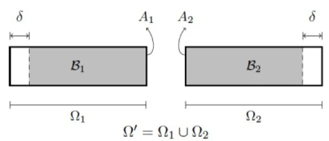
is the micromodulus function, which represents the spring stiffness of the material, and [a ,b ] is an extension of the domain [ , ]a b introduced above, as illustrated in Figure 1.
Clearly, if a and
b
, then
'
and the equilibrium equation (8) has the same form of the one-dimensional equilibrium equation presented by Silling et al. (2003) for an infinite bar made of a linear elastic material with a micromodulusC
s( )
. There, however,C
s( )
may not vanish for | | . Also, the expression (8)is the governing equation of a bond-based peridynamic material, since it does not take into account the collective deformation of points in a
-neighborhood of a pointx
.Figure 1: Domain
and its extension
.Even though the concept of stress is not essential in peridynamics, we define below a normal stress function ( )x
, which is used to relate the micromodulus function C( ) , given by (9), to the Young’s modulus
E
in the classical linear elasticity. For this, consider a perpendicular cross section of the cylindrical bar at an arbitrary pointx
and letA
1 andA
2be, respectively, the left and the right cross sections, as illustrated in Figure 2. In addition,
(1) (1)
(2) (2)
1 x |x x , 2 x |x x ,
(10)
and let
i, i 1,2, be the part of the bar corresponding to
i.Figure 2: The domains
1 and
2 that arise from the imaginary cut at x.Recall from classical continuum mechanics that the normal stress at the surface
A
1 is the normal force per unit area exerted across the cross section upon the material on the surfaceA
1 by the material on the surfaceA
2. Since peridynamics is a non-local theory, not only points inA
2 but also points in
2 exert forces in
1.In the one-dimensional theory, we take the normal stress ( )x to be the sum of all resultant forces of the form (2) (1)
( ,
)
F x x
that a point (2 ) 2x exerts on a point (1) 1
x . Here,
(2) (1) (1) (2) (1) (2) (1) (2) (1) (2)
1 2
ˆ ˆ
( , ) ( ) ( ) , , .
F x x T x h x x T x h x x x x (11)
It then follows from (4), (6), (7), (9), and (11) that
(2) (1) (2) (1) (2) (1) (1) (2)
1 2
( , ) ( ) ( ) ( ) , , .
F x x C x x u x u x x x (12)
The normal stress function of a peridynamic bar is defined by
1 2
(2) (1) (2) (1)
( )
x
F x
(
,
x dx dx
)
.
(13)Taking x(2) x r for r [0,b x] and x(1) x s for s [0,x (a)], recalling the definitions in
(10), and substituting (12) into (13), we obtain
0 0
( )x
x a
b xC r( s u x) ( r) u x( s dr ds) . (14)
We now consider a homogeneous deformation, for which u x( )x, and rewrite (14) as
1 2
0 0
( )x
C r( s r) s dr ds, (15)
where
1
x
(
a
)
and
2
b
x
. We present computational results in Section 4 that justify the use of homogeneous deformation in (14). By making the change of variable v r( ) r s for a fixed s in the inner integral of (15), we rewrite this expression as1 2
0
( ) s ( ) .
s
x
C v vdvds (16)
{
( , )v s 2 | ( , )v s s s, 2 0, 1}
,
which can be written as
1
2
3,
with
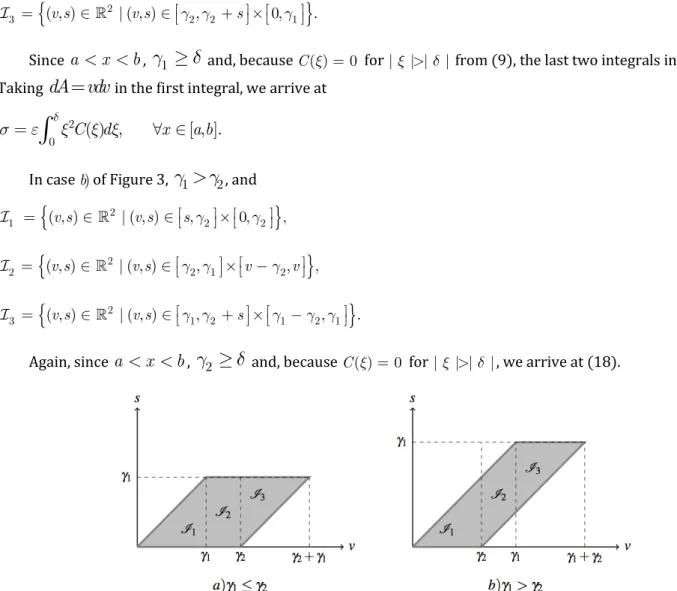
i, i 1,2,3, being a subdomain falling into one of the two cases depicted in Figure 3, which are given by1 2
)
a
andb
)
1
2. We then have from (16) that 3 1 ( ) ( ) . i i
x C v vdA
(17)
In case a) of Figure 3,
1
2, and
21 1 1
2
2 1
1
2 1
2
3 2 2
( , ) | ( , ) , 0, ,
( , ) | ( , ) , 0, ,
( , ) | ( , ) , 0, .
v s v s s
v s
s v s
v s v s
Since
a
x
b
,
1
and, because C()0 for | | | | from (9), the last two integrals in (17) vanish. TakingdA vdv
in the first integral, we arrive at2
0 C d( ) , x [ , ].a b
(18)
In case b) of Figure 3,
1
2, and
2 1 2 22 2 2
2
3 2 1 2
2
1
1 1
( , ) | ( , ) , 0, ,
( , ) | ( , ) , , ,
( , ) | ( , ) , , .
v s v s s
v s v s v v
s v s v s
Again, since
a
x
b
,
2
and, because C() 0 for | | | | , we arrive at (18).On the other hand, ( )x E, x [ , ]a b , from classical elasticity, where
E
is the Young's modulus. It then follows from (18) that2 0 ( ) ,
E
C d (19)which establishes a relation between the Young’s modulus from classical theory and the micromodulus function from peridynamics.
Silling et al. (2003) have obtained an analogous relation between an even micromodulus function, denoted here by
C
S( ),
and the Young's modulus of an infinite bar. Their relation is given by2
0 S( ) .
E
C d (20)If
C
S( )
has the form given by (9), then both expressions (19) and (20) are equivalent in the case of an infinitebar.
Substituting (9) into (19) and using (7), we find that 2 1 /
c E m , which can be inserted back into (9) to yield 2 (| |)
if | | , ( )
0, otherwise.
E
C m
(21)
3 FINITE BAR PULLED AT THE ENDS
Now, let us consider a linearly elastic bar of length
L
in its natural state and take a 0 ,b L
, so that(0, )L
and [ ,L]. The bar is in equilibrium with no body force, so that the equation (8) becomes ( )[ ( ) ( )]d 0, (0, ).
L
C x x u x u x x x L
(22)On the extended parts of the bar, we impose displacement boundary conditions given by
( )
( ) for
[
, ]
0
L,L
.
u x
u x
x
(23)We then have that the problem of equilibrium without body force of the peridynamic bar consists of finding the axial displacement u: (0, )L that satisfies the equilibrium equation (22) together with the boundary conditions given by (23).
Now, let
0 ( )d
C C
(24)
and observe from (22) that
0
0 0
0
0 ( ) ( )d ( )
( ) ( )d ( ) ( ) ( )d ( ) ( )d . L
L L
L
C x x u x x C u x
C x x u x x C u x C x x u x x C x x u x x
This can be rewritten in the form
0 0 0
( ) 1
( ) ( ) ( )d , (0, ),
L
g x
u x C x x u x x x L
C C
where
0
( ) ( ) ( )d ( ) ( )d .
L
L
g x C x x u x x C x x u x x
(26)
The integral equation (25) together with (26) yield an inhomogeneous Fredholm equation of the second kind, where the role of the kernel is played by the micromodulus function and the function g x( ) depends only on the boundary data. Conditions for existence of solutions are associated with the form of the kernel (see, for instance, Porter and Stirling (1990)). Granted that a solution exists, the equation can be easily solved numerically. Recall from Section 1 that a Fourier transform technique is used to find a closed form solution for the case of infinite domains. In the next section we introduce different expressions for the micromodulus function and solve numerically the problem defined by the governing equation (22) together with the boundary conditions (23).
4 NUMERICAL RESULTS
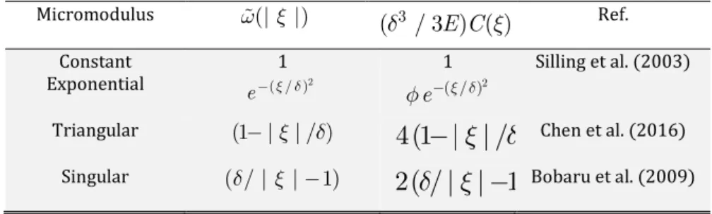
We consider four different expressions for the influence function (| |) that appears in (21) together with (7). They are listed in Table 1 together with the corresponding non-zero parts of the micromoduli C( ) .
Table 1: Expressions for the micromodulus C( ) , where ( 2 e Erf(1)) / 3 1.7593 1. Micromodulus (| |) ( / 3 ) ( )3 E C Ref.
Constant 1 1 Silling et al. (2003)
Exponential ( / )2
e ( / )2
e
Triangular (1 | | / )
4(1 | | / )
Chen et al. (2016) Singular ( / | | 1)2( / | | 1)
Bobaru et al. (2009)Observe from Table 1 that we have also included the reference where, to the best of our knowledge, the corresponding expression first appeared. Concerning the exponential micromodulus, Mikata (2012) has introduced an analogous expression for a bar of infinite length, where 4 / (3 ). Exponential functions are also used in the work of Kilic and Madenci (2010). The constant and the triangular micromoduli correspond to, respectively, the constant and the triangular micromoduli with n 0 in Chen et al. (2016) and the singular micromodulus
corresponds to the triangular micromodulus with
n
1
also in Chen et al. (2016).In all cases, the micromoduli are proportional to
E
in the interval ( , ) and zero elsewhere. It follows from either (22) or (25) together with both (24) and (26) that the numerical results do not depend on the value ofE
and, therefore, this value will be ignored in the following computations.The particularly simple form of the expression (22) allows a straightforward implementation of a numerical scheme, which can be extended to higher dimensions, for the numerical calculation of the displacement field of the peridynamic bar. An alternative numerical scheme2, based on the Fredholm equation (25) together with both (24) and (26), has also been implemented, but will not be presented here. Considering the boundary conditions
1 1 2
( ) x t
x
Erf x e dt
is the Gauss error function.0 if ( ,0), ( )
if ( , ),
x u x
x L L
(27)
we first introduce the new variables
x
xL
and u u/, where, now, x (0,1) and u x( )(0,1), into (22) and rewrite this expression as0
0
1
(( ) )[ ( ) ( )]d 0, [0, ,1]
l
l
C x x L u x u x x x
(28)where we have introduced the definition
L
.In the simplest approach, one can discretize the interval (,1) with
N
1 2
n
equidistant nodes such thatx
n
,x
0
0
,x
N
1
, andx
N n
1
. We then have that the distance between nodes is constant and given by h 1 /N /n and that the discretized form of the equilibrium equation (28) becomes the system of1
N
equations(( ) )[ ( ) ( )] 0, 0,..., . N n
i j i j
j n
C x x L u x u x h i N
(29)In this work we consider geometric sequences of nodes starting with both
N
1000
andn
20
and having a factor of2
. Substituting C( ) , given by one of the expressions in Table 1, into the system of equations (29), we can solve foru x
( ),
ii
0, , ,
N
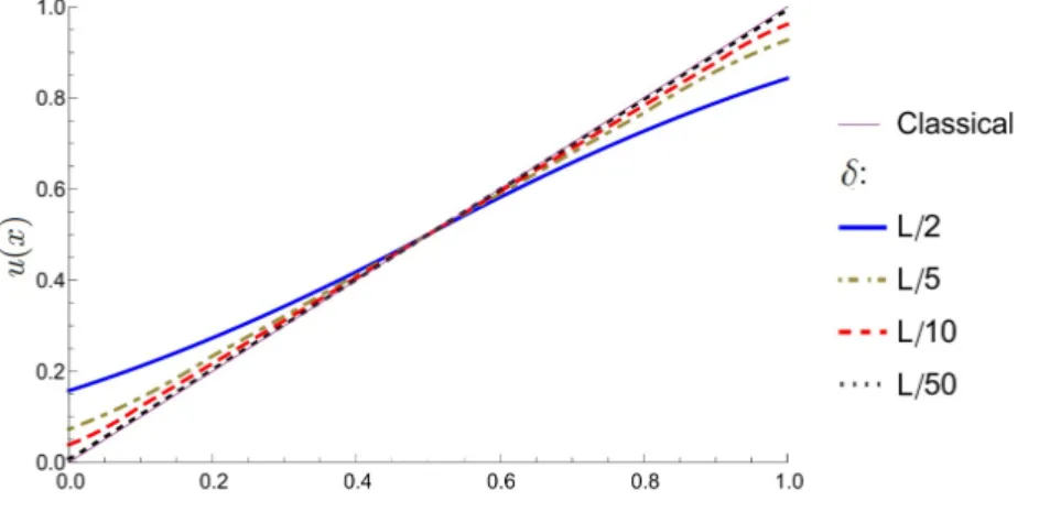
and obtain an approximate expression for the displacement field u x( ).To investigate the influence of the horizon
on the solution of the integral equation (28), we consider the constant micromodulus given by the first expression in Table 1 and the four horizons1/ 2, 1/ 5, 1/10, 1/ 50
. In Figure 4 we show the displacement u x( ) plotted against the position x (0,1)for these four horizons and
N
16000
nodes, which corresponds to the most refined mesh in this work. Because of the relation 1 /N /n introduced above, we have thatn
320
nodes. We see from this figure that (i) the end points of the graphs tend to the points (0,0) on the left end and (1,1)on the right end of the bar as
decreases; (ii) the solution is highly nonlinear in boundary layers of length
near the ends and almost linear outside these boundary layers. In fact, the sequence of solutions tends to the solution of the corresponding problem in the classical linear elasticity theory as
0
, which is linear and satisfies the boundary conditions exactly. This classical solution is represented by the thin solid line in the figure. Thus, at least outside of the boundary layers, we are justified to use homogeneous deformation in (14) to find a relation between the Young’s modulus and the micromodulus function.We see from these observations that displacement discontinuities appear at the ends of the bar for a fixed
0
. The jumps are finite and decrease as the horizon decreases. Displacement discontinuities have already been observed for infinite peridynamic bars under concentrated loads (see, for instance, Silling et al. (2003), Weckner and Abeyaratne (2005), Mikata (2012)), but have not been reported yet for finite bars subjected to displacement conditions at the ends.The reason for the formation of the discontinuities is clear from the analysis of the field equation Erro! Fonte de referência não encontrada., which expresses, for each particle x (0,1) and the corresponding set of particles in its
-neighborhood, the equilibrium of the forces exerted by the particles on the left- and right-hand sides of x. Thus, for a particle located atx
0
, the particles on the interval ( ,0) cannot move and the resultant of the forces on the left hand side must be in equilibrium with the forces on the right-hand side, producing a strain localization. Then, as x 0, we have from the left-hand side that 0C x(( x L u x) )[ ( ) u x x( )]d [3 / ( ) ] ( )E L u x3
from the right-hand side that 3
0C x( x u x)[ ( ) u x x( )]d [3 / ( ) ](E L 0 u x x( )d u x( ) )
. We then have that0
(0 ) ( )d / (2 ) u u x x
, that is, the limit value of u x( ) at the origin from the right-hand side is half of the average of the displacement field evaluated on the right-hand side of the origin. An analogous argument holds for1
x
.Figure 4: Displacement u x( ) versus position x (0,1) obtained from classical linear elasticity and from peridynamics for the constant micromodulus,
N
16000
, and four values of the horizon
.We now show that the field equation (28) converges to the second order ordinary differential equation of classical linear elasticity as
0
for the case of the constant micromodulus. Such demonstration is usually done by using linear displacements as test functions (see, for instance, Silling et al. (2003), Mikata (2012)). Here, however, it is done directly. For x (0,1), straightforward applications of the l'Hôpital rule yield1 3 3 0 0 2 0 0 0 3
0 lim (( ) )[ ( ) ( )]d lim ( )d 2 ( )
lim [ ( ) ( )] 2 ( ) lim [ ( ) ( )] 2
lim [ ( ) ( )] ( ). 2
(
)
(
)
x x EL C x x L u x u x x u x x u x
E E
u x u x u x u x u x
E
u x u x Eu x
(30)Next, we consider the four micromoduli given in Table 1, the horizon 1 / 50 and, again,
N
16000
nodes. We then show in Figure 5 the displacement u x( ) plotted against the reference position x (0, 0.006). For comparison purposes, we also show a graph for the displacement u x( ) obtained from the exact solution of the bar problem in the context of the classical linear elasticity theory. Observe from this figure that all the curves obtained from peridynamics are above the curve obtained from the classical theory, are almost parallel to each other away from the origin, and tend to different values as we approach the origin from its right-hand side. Following arguments that are similar to those presented above in the analysis of the constant micromodulus case, we have verified that these values are approximations of the expression
( ) (( ) ) ( ) (( ) )
0 0
0 d 2 d
u
C xx L u x x
C xx L x
.
In the case of the singular micromodulus, we can rewrite this expression in the form
0 0
(0 ) (( ) )[ ( ) (0 )]d (( ) )d ,
u C x x L u x u x C x x L x
and, provided that
u
(0 )
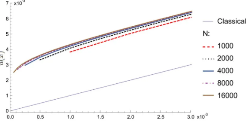
is finite, observe that the integrand in the numerator is less singular than the integrand in the denominator, which tends to infinity as x 0. Thus, we have that u x( )0 as x 0. Also, at least outside of the boundary layers, we are again justified to use homogeneous deformation in (14).From now on, we consider the singular micromodulus only, which is given by the last expression in Table 1. To investigate convergence of the numerical scheme, we show in Figure 6 the displacement u x( ) plotted against the reference position x (0, 0.003) for increasing numbers of nodes and for the horizon 1 / 50. Again, for comparison purposes, we also show the curve obtained from the exact solution of the bar problem in the context of the classical linear elasticity theory. We see from this figure that all the curves obtained from peridynamics are nearly parallel to the curve obtained from the classical linear theory away from the origin, the displacement fields obtained from peridynamics converge to a limit field as the number of nodes increases geometrically, and this limit field seems to have unbounded derivative at x 0 . Convergence to a limit field that is not the classical solution has
been reported in the literature. See, for instance, Bobaru et al. (2009) and Chen et al. (2016).
To verify the unbounded derivative of the limit function, we have considered a node at
x
0
and its immediate neighbor on its right-hand side and evaluated the relative position
x
between the two nodes as well as their relative displacement
u
for the fixed value 1 / 50 and for eachN
shown in Figure 6. We have then obtained Figure 7 showing graphs of the ratio
u
/
x
versus x (0, 0.003) for increasing values ofN
. A diamond symbol on the curves yield the position of the first node to the right of the origin corresponding to a discretization with the number of nodes shown next to the symbol. We then see from the figure that all the curves are on the top of each other for x0.001, which corresponds to the position of the first node in a discretization with1000
nodes. We also see that the ratio
u
/
x
becomes unbounded as the mesh becomes refined, with the curves corresponding to less refined meshes being indistinguishable from the curve corresponding to a more refined mesh.Figure 5: Displacement u x( ) versus position x (0, 0.006) obtained from classical linear elasticity and from peridynamics for 1 / 50, N 1 6 0 0 0 , and four different micromoduli
C
.In Figure 8 we hold
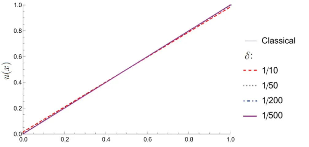
N
16000
fixed and show the displacement u x( ) plotted against the reference position (0,1)x for increasing values of the horizon
. Again, for comparison purposes, we also show the curve obtained from the classical linear elasticity theory. Observe from this figure that the peridynamic solutions tend to the classical solution as
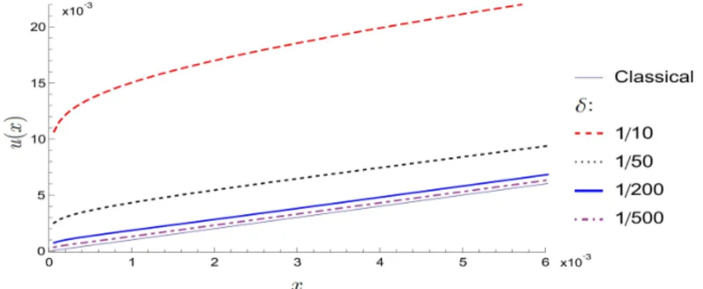
decreases. To investigate the behavior of these curves near the origin, we have plotted Figure 9, which shows u x( ) against x in the interval (0, 0.006). Observe from this figure that u x( ) obtained from peridynamics is highly nonlinear near the origin, tends to u x( ) obtained from classical theory as
0
, and, as observed earlier, seems to have unbounded derivative at x 0 .Figure 7: Ratio between relative displacement
u
and relative position
x
versus position x (0, 0.003) obtained for the case of singular micromodulus, 1 / 50, and an increasing number of nodesN
.Figure 8: Displacement u x( ) versus position x (0,1) obtained from classical linear elasticity and from peridynamics using
N
16000
and decreasing values of the horizon .5 DISCUSSION AND CONCLUSIONS
Figure 9: Displacement u x( ) versus position x (0, 0.006) obtained from classical linear elasticity and from peridynamics using
N
16000
and decreasing values of the horizon .We have then investigated the one-dimensional problem of a linear elastic peridynamic bar of finite length
L
in equilibrium with no body force being pulled at the ends by imposed displacements on extended parts of the bar, which have length
. We have shown that the problem can be formulated in terms of an inhomogeneous Fredholm equation of the second kind. We have then used a numerical scheme to obtain approximate solutions for the peridynamic problem using different expressions of micromodulus, horizons, and discretizations. Except for the singular micromodulus, all the other micromoduli yield discontinuous displacements at the ends of the bar. Discontinuous displacements have been reported in the study of infinite bars, but not of finite bars. The singular micromodulus gives continuous displacements with unbounded derivatives at these ends. In addition, in all cases we have observed homogeneous deformations outside a boundary layer near the ends of the bar. This observation justifies our approach of using homogeneous deformation in (14) to find a relation between the Young’s modulus and the micromodulus function.We have then focused our attention in the investigation of the singular case and found that the approximate solutions of the peridynamic problem converge to the classical solution of linear elasticity for vanishing horizon and a fixed discretization. Also, for a fixed horizon, these solutions converge to a limit function as the grid spacing,
h
, tends to zero. The information obtained from the investigation of the one-dimensional peridynamic problem can now be applied to better understand the behavior of solutions in higher dimensions and to design effective numerical schemes for higher-dimensional problems.6 ACKNOWLEDGEMENTS
The first and fourth authors acknowledge the support of CNPq, under grant 444896/2014-7. The second author acknowledges the support of FAPESP, under grant 2016/12529-4. The third author acknowledges the support of FAPESP, under grant 2016/12217-2, and the partial support of the Italian Ministry, under grant MIUR-PRIN voce COAN 5.50.16.01 code 2015JW9NJT.
References
Aguiar, A.R. (2016). On the Determination of a Peridynamic Constant in a Linear Constitutive Model. Journal of Elasticity, 122(1):27–39. Erratum to: On the Determination of a Peridynamic Constant in a Linear Constitutive Model. Journal of Elasticity, 122(1):41–42.
Aguiar, A.R., Fosdick, R. (2014). A constitutive model for a linearly elastic peridynamic body. Mathematics and Mechanics of Solids, 19:502–523.
Bobaru, F., Yang, M., Alves, L., Silling, S., Askari, E., Xu, J. (2009). Convergence, adaptive refinement, and scaling in 1D peridynamics. International Journal for Numerical Methods in Engineering, 77(6):852–877.
Kilic, B., Madenci, E. (2010). An adaptive dynamic relaxation method for quasi-static simulations using the peridynamic theory. Theoretical and Applied Fracture Mechanics 53:194–204.
Mikata, Y. (2012). Analytical solutions of peristatic and peridynamic problems for a 1D infinite rod. International Journal of Solids and Structures, 49(21):2887–2897.
Nishawala, V., Ostoja-Starzewski, M. (2017). Peristatic solutions for finite one- and two-dimensional systems. Mathematics and Mechanics of Solids, 22(8):1639–1653.
Porter, D., Stirling, D. (1990). Integral Equations: A Practical Treatment, from Spectral Theory to Applications. Vol. 5. Cambridge University Press, Cambridge, UK.
Queiruga, A.F., Moridis, G. (2017). Numerical experiments on the convergence properties of state-based peridynamic laws and influence functions in two-dimensional problems. Comput. Methods Appl. Mech. Engrg. 322:97–122.
Seleson P., Parks M.L., (2011). On the role of influence function in the peridynamic theory. International Journal for Multiscale Computational Engineering, 9(6):689–706.
Silling, S., Epton, M., Weckner, O., Xu, J., Askari, E. (2007). Peridynamic states and constitutive modeling. Journal of Elasticity, 88(2):151–184.
Silling, S., Zimmermann, M., Abeyaratne, R. (2003). Deformation of a peridynamic bar. Journal of Elasticity, 73(1):173--190.
Wang, L., Xu, J., Wang, J. (2017a). Static and dynamic Green's functions in peridynamics. Journal of Elasticity, 126(1):95--125.
Wang, L., Xu, J., Wang, J. (2017b). Erratum to: Static and dynamic Green's functions in peridynamics. Journal of Elasticity, 126(1):127--128.
Weckner, O., Abeyaratne, R. (2005). The effect of long-range forces on the dynamics of a bar. Journal of the Mechanics and Physics of Solids, 53(3):705–728.