www.atmos-chem-phys.net/7/4001/2007/ © Author(s) 2007. This work is licensed under a Creative Commons License.
Chemistry
and Physics
GEM/POPs: a global 3-D dynamic model for semi-volatile persistent
organic pollutants – Part 1: Model description and evaluations of air
concentrations
S. L. Gong1,2, P. Huang1, T. L. Zhao2, L. Sahsuvar1, L. A. Barrie4, J. W. Kaminski3, Y. F. Li1, and T. Niu5
1Air Quality Research Division, Science & Technology Branch, Environment Canada, 4905 Dufferin Street, Toronto, Ontario
M3H 5T4, Canada
2Department of Chemical Engineering and Applied Chemistry, University of Toronto, 200 College Street, Toronto, Ontario,
Canada, M5S 3E5, Canada
3Department of Earth and Space Science and Engineering, York University, 4700 Keele Street, Toronto, Ontario, M3J 1P3,
Canada
4Atmospheric Research and Environment Program, World Meteorological Organization, 7 bis, avenue de la Paix, BP2300,
1211 Geneva 2, Switzerland
5Certre for Atmosphere Watch & Services (CAWAS), Chinese Academy of Meteorological Sciences, China Meteorological
Administration (CMA), Beijing 100081, China
Received: 19 January 2007 – Published in Atmos. Chem. Phys. Discuss.: 2 March 2007 Revised: 30 May 2007 – Accepted: 12 June 2007 – Published: 1 August 2007
Abstract. GEM/POPs was developed to simulate the trans-port, deposition and partitioning of semi-volatile persis-tent organic pollutants (POPs) in the atmosphere within the framework of Canadian weather forecasting model GEM. In addition to the general processes such as anthropogenic emis-sions, atmosphere/water and atmosphere/soil exchanges, GEM/POPs incorporates a dynamic aerosol module to pro-vide the aerosol surface areas for the semi-volatile POPs to partition between gaseous and particle phases and a mech-anism for particle-bound POPs to be removed. Simulation results of three PCBs (28, 153 and 180) for the year 2000 indicate that the model captured the main features of global atmospheric PCBs when compared with observations from EMEP, IADN and Alert stations. The annual averaged con-centrations and the fractionation of the three PCBs as a func-tion of latitudes agreed reasonably well with observafunc-tions. The impacts of atmospheric aerosols on the transports and partitioning of the three PCBs are reasonably simulated. The ratio of particulate to gaseous PCBs in the atmospheric col-umn ranges from less than 0.1 for PCB28 to as high as 100 for PCB180, increasing from the warm lower latitudes to the cold high latitudes. Application of GEM/POPs in a study of the global transports and budgets of various PCBs accompa-nies this paper.
Correspondence to:S. L. Gong ([email protected])
1 Introduction
Persistent organic pollutants (POPs) are organic chemical compounds and mixtures that include industrial chemicals like PCBs, pesticides like DDT and by-products of combus-tion like dioxins. Due to their resistance to degradacombus-tion in the environment, POPs have long half-lives. Successive re-leases of these chemicals over time have resulted in contin-ued accumulation in the global environment and posed a risk of causing adverse effects to human health and the environ-ment. POPs released to the atmosphere with various physic-ochemical properties have substantial difference in their be-haviours in the environment. As a result of the tendency of POPs to move from warmer to colder environment even the Arctic ecosystem is exposed to some POPs at levels of con-cern (Halsall, 2004; Hung et al., 2002). Due to POPs’ ability to accumulate in various natural media, an evaluation of con-tamination by POPs requires a multi-compartment approach that includes atmosphere, soil and water.
in demonstrating the “grasshopper” effect. However, these (multimedia) models are less suitable to predict the detailed spatial and short-term variability in the distribution of a com-pound. To overcome the limitation of box-type models, dy-namical 3-D models have been developed to describe the atmospheric transport of POPs on both regional (Ma et al., 2003; van Jaarsveld et al., 1997), hemispheric (Gusev et al., 2005; Hansen et al., 2004) and global scales (Koziol and Pudykiewicz, 2001; Semeena and Lammel, 2005; Strand and Hov, 1996). These models include meteorological pa-rameters such as wind speed, temperature and precipitation rate in finer spatial and temporal resolutions for more accu-rate transport, chemical reactions and removal processes of POPs. Species that have been simulated in these models in-clude PCBs, DDTs and HCHs.
3-D dynamic models also make it possible to more realis-tically treat the phase partitioning of semi-volatile POPs be-tween gaseous and particulate phases, which strongly influ-ences the transformation, transport and fate of PCBs in the environment (Sahsuvar et al., 2003). The removal of a PCB from the atmosphere is very different if it is bound to parti-cles than if it is in the gas phase. Thus it is essential to model PCB pathways in the atmosphere using a model that realisti-cally simulates aerosols. Previous studies of POPs either deal with more volatile compounds such as HCH (Hexachlorocy-clohexane) (Hansen et al., 2004; Koziol and Pudykiewicz, 2001) or use prescribed aerosol distributions for parameteriz-ing partitionparameteriz-ing for semi-volatile POPs (Gusev et al., 2005). The dynamic features of atmospheric aerosols were not re-alistically provided to properly simulate the semi-volatile POPs in the atmosphere. Semmna et al. (2006) studied the impact of climate and substance properties on the fate and atmospheric long-range transport of DDT andγ-HCH with an interactive aerosol module and portioning schemes. How-ever, no substantial insights on the impact of the partitioning were discussed.
GEM/POPs is a 3-D global POPs transport model com-posed of two major components: (1) a multiscale air qual-ity model (GEM-AQ) which includes a weather forecast model with on-line gas phase chemistry, an aerosol mod-ule CAM (Canadian Aerosol Modmod-ule) and (2) a POPs ex-change and partitioning module for atmosphere/water, atmo-sphere/soil exchanges and partitioning of POPs between gas and aerosols. This paper describes the modelling system and evaluates the performance with available observations of global PCBs. As a further application of GEM/POPs, the global transports and budgets of PCBs are simulated for three typical congeners that range from volatile (PCB28) to semi-volatile (PCB153 and PCB180) species, which is presented in the companion paper (Huang et al., 2007).
2 Model description
2.1 GEM-AQ
GEM (Global Environmental Multiscale model) (Cˆot´e et al., 1998) was developed at MSC (Meteorological Service of Canada) for operational weather forecasting applications. GEM-AQ adds on a gas phase chemistry module (ADOM) (Venkatram et al., 1988) and an aerosol module (CAM) (Gong et al., 2003), which produces a 3-D global OH dis-tribution for POP gas phase chemistry and a global aerosol surface area distribution for semi-volatile POP partitioning, respectively. Because of the inclusion of major atmospheric processes and types of aerosols in the CAM (Gong et al., 2003), the particle-bound removal rate of any semi-volatile POPs is treated as same as the particles.
2.2 Atmospheric Processes of POPs
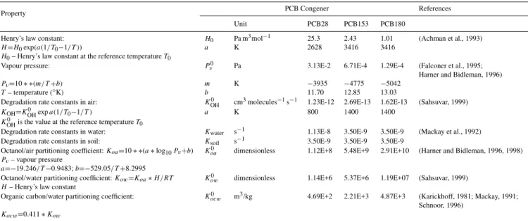
In addition to the large scale transport of POPs by general cir-culation and turbulent mixing provided by GEM, GEM/POPs implemented the atmospheric processes of gas phase oxida-tion, exchanges between water/soil and atmosphere, and par-titioning between particle and gas. The description of these processes is demonstrated with PCBs and the physiochemi-cal properties of the 3 PCBs simulated in this study are listed in Table 1. To apply GEM/POPs to other POPs, the phys-iochemical properties, chemical reaction rate constants and emission fields of a specific POPs are needed.
2.2.1 Oxidation
It has been experimentally shown by several groups that the gas phase PCBs undergo homogeneous degradation by pho-tolysis and reaction in the atmosphere dominantly with the hydroxyl (OH) radicals but also with NO3 radicals and O3
(Anderson and Hites, 1996; Atkinson and Aschmann, 1985; Kwok et al., 1995). The OH reactions occur via addition to the biphenyl ring to replace chlorine atoms and to form vari-ous isomers of (PCB·OH):
PCB+ ·OH→PCB·OH (1)
and ∂CPCB/∂t=−kOH×COH×CPCB (2)
Assuming [OH] is constant, the integration gives
ln(CPCB/CPCB,o)= −kOH×COH×t = −k′OH×t (3)
with logkOH=−0.22∗(#Cl)−11.25 (4)
where,CPCB,o is the initial PCB concentration,t(s) is time, kOH(cm3/molecule.s) is the rate constant for PCB-OH
reac-tion,k′ OH(s
−1)is the pseudo-first order rate constant, and #Cl
Table 1.Physicochemical properties of three PCB congeners and their temperature dependent parameters.
T = temperature (◦K),T
0= reference temperature (298◦K),R= gas constant.
Property PCB Congener References
Unit PCB28 PCB153 PCB180
Henry’s law constant: H0 Pa m3mol−1 25.3 2.43 1.01 (Achman et al., 1993)
H=H0exp(a(1/T0−1/T )) a K 2628 3416 3416
H0– Henry’s law constant at the reference temperatureT0
Vapour pressure: Pv0 Pa 3.13E-2 6.71E-4 1.29E-4 (Falconer et al., 1995;
Harner and Bidleman, 1996)
Pv=10∗ ∗(m/T+b) m K −3935 −4775 −5042
T– temperature (◦
K) b 11.70 12.85 13.03
Degradation rate constants in air: KOH0 cm3molecules−1s−1 1.23E-12 2.69E-13 1.62E-13 (Sahsuvar, 1999) KOH=KOH0 expa(1/T0−1/T ) a K 800 1400 1400
KOH0 is the value at the reference temperatureT0
Degradation rate constants in water: Kwater s−1 1.13E-8 3.50E-9 3.50E-9 (Mackay et al., 1992)
Degradation rate constants in soil: Ksoil s−1 3.50E-9 3.50E-9 3.50E-9
Octanol/air partitioning coefficient:Koa=10∗ ∗(a∗log10Pv+b) Koa0 dimensionless 1.12E+8 5.48E+9 2.91E+10 (Harner and Bidleman, 1996, 1998)
Pv– vapour pressure
a=−19.246/T−0.9483;b=−529.05/T+8.2995
Octanol/water partitioning coefficient:Kow=Koa∗H /RT Kow0 dimensionless 1.14E+6 5.37E+6 1.19E+07 (Sahsuvar, 1999)
H– Henry’s law constant
Organic carbon/water partitioning coefficient: Kocw0 m3/kg 4.69E+2 2.21E+3 4.87E+3 (Karickhoff, 1981; Mackay, 1991; Schnoor, 1996)
Kocw=0.411∗Kow
2.2.2 Atmosphere-water exchange
Atmosphere-water exchange of PCBs was treated with a method by Liss and Slater (1974) characterized by mass transfer coefficients ofkW (water side) andkA(air side). The
dimensionless Henry’s Law constant,KAW, gives the ratio
of the concentrations across the atmosphere-water interface with a flux:
F=KT W(CW−CG/KAW)=KT A(CW×KAW−CG) (5)
where overall mass transfer coefficients KT W (water-side,
s m−1)andK
T A(air-side, s m−1)are:
1/KT W =1/ kW+1/(kA×KAW)=1/ kW+RT /(H×kA) (6)
1/KT A=1/ kA+KAW/ kw=1/ kA+H /(RT ×kW) (7)
Assuming unsteady state, the Eq. (5) is solved to give the gas phase concentration of first model level as:
CG(t )=CW×KAW+(CGO−CW×KAW)exp(−KT A×1t / h0) (8) whereCGO is the initial atmosphere concentration andh0is
the thickness of the first model layer. The water PCB con-centration,CW, is assumed constant for the integration time
step1t but will change after receiving deposition from the atmosphere and transports in oceans. A detailed description of the dimensionless Henry’s Law constant (KAW)and mass
transfer coefficients (kAandkW)is given by (Sahsuvar et al.,
2003) using the data from Table 1.
2.2.3 Atmosphere-soil exchange
An atmosphere-soil exchange model by Jury (Jury, 1989; Jury et al., 1983) was used for calculating the soil PCB fluxes to the atmosphere:
Fnet(0, t )=(CG,soil−CG,air×KSA)
r
DES π×t
"
1−exp −L
2
4DES×t
!#
(9) whereCG,soil and CG,air are the gaseous phase
concentra-tions in soil and atmosphere, respectively,KSA
(dimension-less) is the soil-atmosphere equilibrium coefficient, andDES
(m2s−1)is the effective diffusivity of the chemical (PCBs).
TheDESterm is derived from a series of equations and
par-titioning coefficients: KSAandKAW (Sahsuvar et al., 2003).
In the current GEM/POPs, the soil column with a depth of
Lis divided into three superposed layers: 1 cm surface soil (z1), 3 cm second layer (z2) and 7 cm bottom layer (z3). 2.2.4 Gas-aerosol partitioning
The PCB amount partitioned between gas and aerosol phase depends on the aerosol surface area available for adsorption (m2aerosol/m3 air) and the liquid-phase saturation vapour pressure of pure compound (Pa). PCB/aerosol partitioning was simulated with the Junge-Pankow scheme (Junge, 1977; Pankow, 1987) as:
8= c
×2
PL0+c×2 =
CP
Cp+CG
Table 2. Soil concentrations of three PCBs in China (ng/g dry weight).
Locations Coordinates PCB28 PCB153 PCB180
Chongqing N 29◦33 E 106◦38 24.3 ND ND
Wuhan N 30◦42 E 114◦36 18.4 7.0 7.0
Yichang N 30◦34 E 111◦27 19.4 ND ND
Xian N 33◦84 E 109◦00 23.1 4.7 ND
Beijing N 40◦10 E 117◦18 21.9 12.0 22.2
Inner Mongolia N 43◦14 E 122◦14 14.7 ND ND
ND: Not detectable
where,
8 = fraction of semi-volatile organic compound adsorbed on aerosol particles (Cp andCG are the concentrations of
particle-bound and gaseous PCBs)
c= parameter that depends on the thermodynamics of the adsorption process and surface properties of the aerosol (Pa cm)
2 = aerosol surface area available for adsorption (m2aerosol/m3air)
PL0 = liquid-phase saturation vapour pressure of pure compound(Pa)
Junge’s proposed value of the parameterc is 17.2 Pa cm (Bidleman et al., 1998; Pankow, 1987). Within the GEM/POPs framework, the CAM provides aerosol surface areas (2)dynamically. In addition to the Junge-Pankow ad-sorption scheme adapted in this study,KOA(the octanol-air
partition coefficient) based absorption model has also been used in predicting the phase partitioning of semi-volatile POPs (Finizio et al., 1997; Semeena et al., 2006), such as PCBs, DDT andγ-HCH.
2.2.5 Removal processes
The particulate phase PCBs are removed along with the aerosols by wet and dry deposition which are given in details by Gong et al. (2003). The gas phase PCBs are destroyed by OH radical attack (see Sect. 2.2.1) and removed by precipita-tion scavenging, assuming to be in quasi-steady equilibrium with the rain drop. The net wet deposition flux,Fw, is then
written as
Fw =(−p/KAW)×CG (11)
wherep is the precipitation rate, usually reported in mm/h andCGis the gas phase PCB concentration.
2.3 Ocean/lake transport module
As previously discussed, an atmosphere-water exchange module needs the concentrations of POPs in the water pro-vided by either an ocean/lake module or global observations. In GEM/POPs, an ocean tracer transport module is devel-oped with prescribed global ocean currents from the UK
Ocean Circulation and Advanced Modelling Project (OC-CAM) (de Cuevas, 1999) and with the French OPA tracer model (Foujols et al., 2000). With the 5-day mean oceanic currents from OCCAM as an input, the OPA tracer model computes the evolution of passive tracers and yields the 3-D distributions of POPs in world oceans. For regional simu-lation of POPs such as for the Great Lakes region in North America, a lake module is also needed to study the deposi-tion and re-emission from lakes. Since this study deals with largely global transport features of PCBs, no lake module is included.
2.4 Other processes
In addition to the processes described above, there are other environmental compartments that POPs will be portioned in such as vegetation, ice and sediments (Malanichev et al., 2004). According to Malanichev et al. (2004), the emissions and accumulations of various PCBs from sea-water and veg-etation take only a very small fraction of the total PCBs in the environmental media while the soil compartment is the dom-inant PCB sources in 1995. Consequently, the sea-ice and vegetation compartments are neglected in the current version of GEM/POPs in terms of the accumulation of PCB masses in these compartments. However, the deposition of POPs into these compartments is accounted for as the dry deposi-tion scheme differentiates different land use categories.
3 Input conditions
3.1 Meteorological data
Simulation for the year 2000 was done with the re-analyzed meteorology from CMC (Canadian Meteorological Centre) updated every 24 h to drive the GEM. The model resolution was set at 2◦×2◦ with an integration time step of 15 min.
The results shown in this paper were obtained after 2 years of spin-up runs prior to year 2000.
3.2 Emission data
The historical production of PCBs and chemical composi-tion of various technical mixtures data for 22 PCB congeners from 1930 to 2000 have been compiled from the literature (Breivik et al., 2002a). These data, along with assumptions on the trade between countries and regions, have been uti-lized to derive an estimate of the global historical consump-tion pattern. With a mass balance approach (Breivik et al., 2002b), estimates of the annual emissions of each of the 22 PCB congeners by country and year were obtained. For current simulation, using population density (Li, 1996) as a surrogate, the national consumption or emission data were converted into globe 1◦×1◦emissions where the minimum,
PCB28
PCB153
PCB180
ng/g
Latitude (degree)
60 65 70 75 80 85 90
Con
c
en
tratio
n (fg/L)
0 100 200 300 400 500 600
Observations After Spinning Up/6.0
Before Spinning Up PCB28
Latitude (degree)
60 65 70 75 80 85 90
Con
c
entrat
ion
(f
g
/L)
0 100 200 300 400 500
Observations
After Spinning Up
Before Spinning Up PCB153
Latitude (degree)
60 65 70 75 80 85 90
Co
nce
ntra
tio
n
(fg/L)
0 50 100 150 200 250 300
After Spinning Up
Before Spinning Up Observations PCB180
Fig. 1. (a)Assimilated three PCB soil concentrations from MSC-East hemispheric POP model outputs, soil concentrations (Meijer et al., 2003) and data from China (Table 2). The observed locations and concentrations are expressed as a lined circle filled with the same color scale as the contour plots.(b)Comparisons of the oceanic PCB concentrations used in the model after two years of spin-up simulations.
data is better to reflect the reality than mean and minimum emissions and is therefore used in this study.
3.3 Initial soil and water concentrations
Current systematic measurements of oceanic and soil PCBs are very limited to form an accurate picture of global distri-butions even though there exist some data of global soil con-centrations (Meijer et al., 2003). Consequently, the model simulation results of both soil and oceanic concentrations of PCBs from the MSC-East hemispheric POP model (Gu-sev et al., 2005) were used to provide the required spa-tial distributions but the magnitudes of soil PCB concen-trations differ substantially from the observations (Meijer et
Initial oceanic PCB concentrations were also evaluated against available observations. After two years of spin-up from the MSC-East model outputs, the sea water concentra-tions match the observaconcentra-tions (Sobek and Gustafsson, 2004) very well for PCBs 156 and 180 (Fig. 1b) along the cruise ship track. Magnitudes and trends of these two PCBs along the latitude direction were reasonably reproduced. For PCB 28, the latitude trend was produced but about 6 time over-estimates for the oceanic surface concentration were pro-duced (Fig. 1b).
4 Simulation results of global PCBs
4.1 Comparisons with observations
There are two types of monitoring data sets for global PCB distributions that are obtained from active and passive sam-plers, respectively. Active measurements use a high volume sampler that takes air through a filter. POPs’ concentrations are then analyzed from the deposits on the filter. This type of technique has been used in a number of international, long-term monitoring programs such as NCP (Northern Contam-inant Program), EMEP (Co-operative Programme for Moni-toring and Evaluation of the Long-range Transmission of Air pollutants in Europe) and IADN (the Integrated Atmospheric Deposition Network). Trends and spatial distributions have been obtained from these sites. Recently, passive air sam-pler types have been developed and used in air monitoring of POPs (Harner et al., 2006). These samplers are small and relatively inexpensive and simple to deploy. Initial data set has been used to evaluate some modeling results (Shen et al., 2006). However, due the nature of the passive sampling, longer sampling time is needed than the active samplers and consequently temporal resolution of the data is rather coarse, i.e. one data per 2 to 7 months. Most of the data from the passive sampling network were not available before 2004. Since this study was focused on year 2000, only data from the active sampling networks were used to compare with the modeling results.
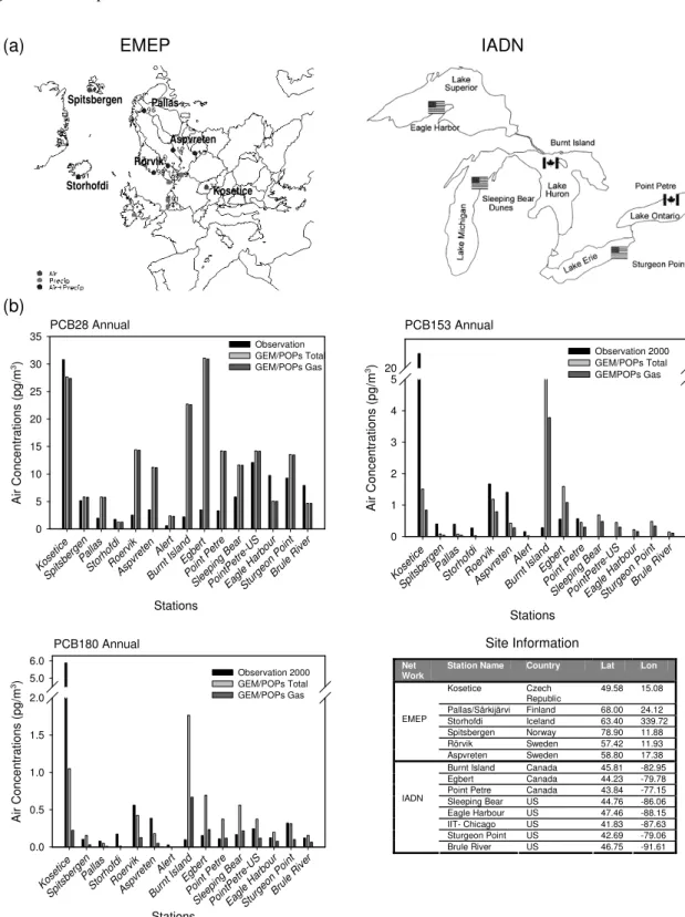
Three major observational data sets of PCB atmo-sphere/particulate concentrations by active samplers were used in the comparison study: EMEP, IADN and Alert/Arctic, representing the European, the Great Lakes re-gion (North America) and Arctic environments, respectively (Fig. 2a). The EMEP stations use very different sampling fre-quencies at various locations raging from one day/two days a week, one week a month, biweekly to monthly without dif-ferentiating gas and aerosol PCBs1. A monthly mean value of total PCBs for each station was given based on the sam-pling data by a high volume sampler. In IADN stations (Sun et al., 2006), the sampling frequency was 1 in 6 days before April 1994 and then switched to 1 in 12 days. Except for 1995, only gaseous PCBs were analyzed. The Alert station
1http://www.nilu.no/projects/CCC/onlinedata/pops/index.html
uses a high volume sampler with weekly integrated sampling and results in four weekly averaged data per month. Since the observed particle-bound concentrations are usually below method detection limits or too erratic to allow for a meaning-ful comparison to the modeled results, only gaseous PCBs were utilized for the study. Consequently, for the annual and monthly concentration comparisons, simulation results for total PCBs will be used at the EMEP stations while only gaseous PCBs at the IADN and Alert stations.
Figure 2b shows the comparisons of model and observa-tions in selected staobserva-tions with annual averaged concentra-tions of both total and gaseous PCBs. A general agreement between modelled and observed PCBs is achieved with re-spect to the relative magnitudes of three different PCBs with the highest air concentration of PCB28 from 5 to 30 pg m−3
while the less volatile PCB153 and PCB180 have a smaller concentration ranging from around 1 to 0.1–0.5 pg m−3,
re-spectively.
Total PCB28 simulated by GEM/POPs at EMEP sta-tions agreed reasonably well with observasta-tions except at two Swedish sites: Aspvreten and R¨orvik, where some overes-timates were made. Two stations at IADN network also showed large over-estimates of gaseous PCB28: Burnt Is-land and Egbert. It is also noted that for the same station of Point Petre, the analysis done separately by the Canadian and American laboratories yielded very different results with the modeling results closer to the American analysis.
No PCB153 was analyzed at the American IADN sites. For EMEP and Canadian IADN sites, the comparison of both PCB153 and PCB180 is reasonable with two exceptions: Kosetice in Czech Republic and Burnt Island in Canada. The extreme high concentrations of PCB153 and 180 observed at the Kosetice site over the entire monitoring period (Fig. 3a) were not simulated. Compared to other European stations, this may imply the existence of some local PCB sources that were not accounted for in our emission inventories. On the contrary, the GEM/POPs predicted higher concentrations of gaseous PCB153 and PCB180 at Burnt Island than the IADN observations.
For the Arctic Alert, long records of PCBs (Hung et al., 2005a) have been obtained through the NCP (Northern Con-taminant Program), indicating a decline trend for various PCBs (Hung et al., 2005b). The modeling results show a good agreement of the magnitudes of three modeled PCBs for year 2000 (Fig. 2b) with slightly overestimate of PCB28 and under-estimates of PCB153 and 180.
(a) EMEP
Spitsbergen Pallas Storhofdi Kosetice Aspvreten RörvikIADN
(b)
PCB28 Annual Stations Koset ice Spi tsber gen Pallas Storhof di Roer vik Aspv rete n Ale rt Burnt Islan d Egber t Poi nt Pet re Sleep ing Bear Point Petr e-US Eagle Harbou r Stur geo n Point Brule Ri ver Air Con c entrations (p g/m 3) 0 5 10 15 20 25 30 35 Observation GEM/POPs Total GEM/POPs Gas PCB153 Annual Stations Kose tice Spits berg en Pal las Sto rho fdi Roerv ik Aspv reten Alert
Burnt Isl and
Egbert Point Petre
Sle epin g B ear Poin tPetre-U S Eagle Harb our Stu rgeon P
oint
Bru le R
iver Air Conce n tratio ns (pg /m 3) 0 1 2 3 4 5 20 Observation 2000 GEM/POPs Total GEMPOPs Gas PCB180 Annual Stations Kose tice Spitsb erge n Pal las Storho fdi Roervik Asp
vreten Alert
Burnt IslandEgbert
Poi nt P
etre
Sleep ing B
ear
Poi ntPetre-US
Eagl e H
arb our Stu rgeon Poin t Brul e Ri ver A ir Conce n tr at ions ( pg/ m 3) 0.0 0.5 1.0 1.5 2.0 5.0 6.0 Observation 2000 GEM/POPs Total GEM/POPs Gas Site Information Net
Work Station Name Country Lat Lon
Kosetice Czech Republic
49.58 15.08
Pallas/Särkijärvi Finland 68.00 24.12 Storhofdi Iceland 63.40 339.72 Spitsbergen Norway 78.90 11.88 Rörvik Sweden 57.42 11.93 EMEP
Aspvreten Sweden 58.80 17.38 Burnt Island Canada 45.81 -82.95 Egbert Canada 44.23 -79.78 Point Petre Canada 43.84 -77.15 Sleeping Bear US 44.76 -86.06 Eagle Harbour US 47.46 -88.15 IIT- Chicago US 41.83 -87.63 Sturgeon Point US 42.69 -79.06 IADN
Brule River US 46.75 -91.61
Fig. 2. (a)Geographic locations of EMEP and IADN master stations.(b)Comparisons of observed and simulated annual averaged PCB28, 153 and 180 for 2000. Note: The PCB28 concentration from GEM/POPs was scaled down 6 times in the plot.
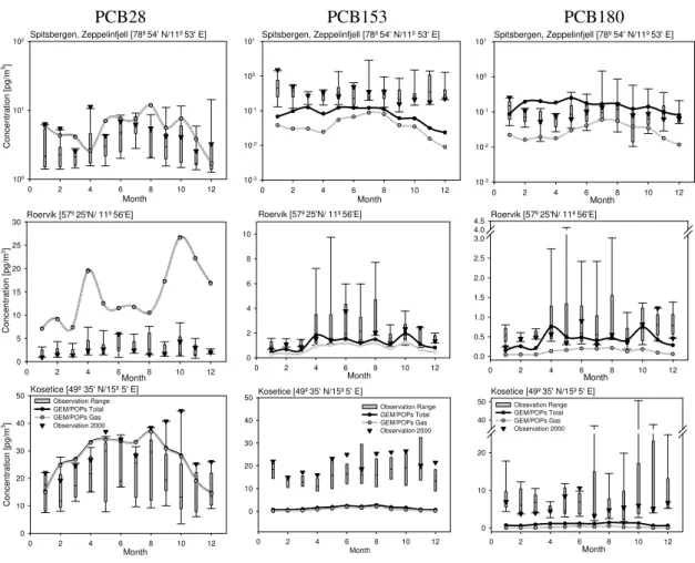
data for several years around 2000, e.g. between 1994–2004 for EMEP sites, 1992–2000 for Alert site and 1993–2003 for IADN, have been used to generate a vertical box to show the variation range of measured PCBs (gray box with whiskers).
(a) EMEP Stations
PCB28 PCB153 PCB180
Spitsbergen, Zeppelinfjell [78º54' N/11º53' E]
Month
0 2 4 6 8 10 12
C
onc
e
ntr
at
io
n [
pg/
m
3]
100
101
102 Spitsbergen, Zeppelinfjell [78º54' N/11º 53' E]
Month
0 2 4 6 8 10 12
10-3
10-2
10-1
100
101 Spitsbergen, Zeppelinfjell [78º54' N/11º53' E]
Month
0 2 4 6 8 10 12
10-3
10-2
10-1
100
101
Roervik [57º25'N/ 11º56'E]
Month
0 2 4 6 8 10 12
Conc
ent
rat
ion [
pg/
m
3]
0 5 10 15 20 25
30 Roervik [57º 25'N/ 11º56'E]
Month
0 2 4 6 8 10 12
0 2 4 6 8 10
Roervik [57º25'N/ 11º56'E]
Month
0 2 4 6 8 10 12
0.0 0.5 1.0 1.5 2.0 2.5 3.0 4.0 4.5
Kosetice [49º 35' N/15º 5' E]
Month
0 2 4 6 8 10 12
Co
ncentr
a
ti
on [pg/m
3]
0 10 20 30 40 50
Observation Range GEM/POPs Total GEM/POPs Gas Observation 2000
Kosetice [49º35' N/15º5' E]
Month
0 2 4 6 8 10 12
0 10 20 30 40 50
Observation Range GEM/POPs Total GEM/POPs Gas Observation 2000
Kosetice [49º35' N/15º5' E]
Month
0 2 4 6 8 10 12
0 10 20 40
50 Obsevation Range GEM/POPs Total GEM/POPs Gas Observation 2000
Fig. 3.Comparisons of modelled and observed three monthly PCBs for 2000 with the measurement range at(a)EMEP;(b)IADN;(c)Alert. The boundary of the box closest to zero indicates the 25th percentile, a line within the box marks the median, and the boundary of the box farthest from zero indicates the 75th percentile. Whiskers (error bars) above and below the box indicate the 90th and 10th percentiles.
measured PCBs. It can also be inferred from the comparisons that there exists a trend of underestimates of heavy PCBs and a trend of over-estimate of lighter PCB28.
For IADN stations where gaseous PCBs were measured, overestimates of gaseous PCB28 concentrations at Point Pe-tre, Burnt Island and Egbert stations were observed. How-ever, a better agreement of PCB28 with American IADN sites was achieved (Fig. 3b). For PCB153 and 180, the com-parison of gaseous phase concentrations reveals a very good agreement for most stations. The magnitudes and summer highs are well simulated except for the Burnt Island site. The PCBs at the Alert station were also reasonably simulated (Fig. 3c). The three PCBs simulated are in the right range of measured values with a summer peak from GEM/POPs at Alert for PCB28 that has not been observed.
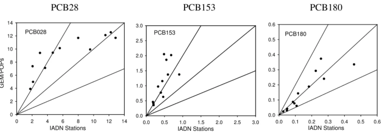
Figure 4 shows the comparisons for the three PCBs be-tween the modeling results from GEM/POPs and the obser-vations averaged over IADN stations for the year 2000. The
predictions for PCB180 are well within a factor of 2 from the observations. However, for PCB28 and PCB153, there are some over-estimates by GEM/POPs but majority of the re-sults are within a factor of 3. The over-estimate is especially evident for PCB153, indicting some systematic bias in the model.
comput-(b) IADN Stations
PCB28 PCB153 PCB180
Point Petre [43.8428º N/ 77.154º W]
Month
0 2 4 6 8 10 12
Conc e n tr at io n [ p g /m 3] 0 5 10 15 20 25 Obaservation Range GEM/POPs Total GEM/POPs Gas Observation 2000
Point Petre [43.8428º N/ 77.154º W]
Month
0 2 4 6 8 10 12
0.0 0.5 1.0 1.5 2.0 2.5 3.0 Obaservation Range GEM/POPs Total GEM/POPs Gas Observation 2000
Point Petre [43.8428º N/ 77.154º W]
Month
0 2 4 6 8 10 12
0.0 0.1 0.2 0.3 0.4 0.5 0.6 0.7 0.8
1.0 Obaservation Range GEM/POPs Total GEM/POPs Gas Observation 2000
Egbert [44.2317º N/ 79.783º W]
Month
0 2 4 6 8 10 12
C o nc en tr a ti o n [ p g /m 3] 0 10 20 30 40 50
60 Egbert [44.2317º N/ 79.783º W]
Month
0 2 4 6 8 10 12
0 1 2 3
4 Egbert [44.2317º N/ 79.783º W]
Month
0 2 4 6 8 10 12
0.0 0.5 1.0 1.5
Eagle Harbour [47.4631º N/ 88.15º W]
Month
0 2 4 6 8 10 12
Co nc en tr ati o n [p g/m 3] 0 5 10 15 20 25
35 Eagle Harbour [47.4631º N/ 88.15º W]
Month
0 2 4 6 8 10 12
0.0 0.2 0.4 0.6 0.8
(c) Alert Station
PCB28 PCB153 PCB180
Alert [82.5º N / 62.3º W]
Month
0 2 4 6 8 10 12
C o n c ent ration [pg/ m 3] 0 2 4 6 8 10 Observation Range GEM/POPs Total GEM/POPs Gas Observation 2000
Alert [82.5º N / 62.3º W]
Month
0 2 4 6 8 10 12
0.0 0.5 3.0 6.0
9.0 Observation Range GEM/POPs Total GEM/POPs Gas Observation 2000
Alert [82.5º N / 62.3º W]
Month
0 2 4 6 8 10 12
0.0 0.1 0.2 0.3 3.0 6.0 Observation Range GEM/POPs Total GEM/POPs Gas Observation 2000
Fig. 3.Continued.
ing the soil-atmosphere exchange fluxes of PCBs over large part of the globe. The other dominant factor that affects the model performance is the uncertainty associated with the an-thropogenic emission data. Besides, the PCB emissions have no seasonal variations and the grid values of each PCB are distributed from the total emission in a country by the popu-lation density. For large countries like Canada and US, this assumption may be subject to very large uncertainties.
4.2 Fractionation of PCBs
PCB28 PCB153 PCB180
PCB028
IADN Stations
0 2 4 6 8 10 12 14
GE
M
/P
O
Ps
0 2 4 6 8 10 12 14
PCB153
IADN Stations
0.0 0.5 1.0 1.5 2.0 2.5 3.0 0.0
0.5 1.0 1.5 2.0 2.5 3.0
PCB180
IADN Stations
0.0 0.1 0.2 0.3 0.4 0.5 0.6 0.0
0.1 0.2 0.3 0.4 0.5 0.6
Fig. 4.Comparisons of three PCBs between the modeling results and the observations averaged over IADN stations for the year 2000.
(
a
)
(
b
)
ANNUAL PCBs FRACTIONATION BY THE LATITUDE (EMEP Stations)
Latitude
45 50 55 60 65 70 75 80 85
FRAC
TION
0.0 0.2 0.4 0.6 0.8 1.0 1.2
Obs. PCB28 Obs. PCB153 Obs. PCB180 GEM/POPs PCB 28 GEM/POPs PCB153 GEM/POPs PCB180
ANNUAL PCBs FRACTIONATION BY THE LATITUDE (IADN Stations)
Latitude
42 43 44 45 46 47 48
FR
ACTIO
N
0.0 0.2 0.4 0.6 0.8 1.0 1.2
Obs. PCB28 Obs. PCB180 GEM/POPs PCB28 GEM/POPs PCB180
Fig. 5.Comparisons of PCB fractionations at(a)Europe and(b)North American stations.
fractions of three atmospheric PCBs as a function of lati-tude for both model simulation and observations in Europe (Fig. 5a) and the fractions of two PCBs in North America (Fig. 5b). PCB28 shows a slightly increasing trend from 50◦N to 80◦N in Europe for both model and observations
with a slope of 0.015 and 0.007, respectively while the heav-ier PCBs of 153 and 180 exhibit an opposite trend with lati-tude in Europe. The slopes for PCB153 and 180 are−0.005 and −0.001 for observations and −0.011 and −0.003 for model simulations. Similar trends of PCBs in soil have also been reported (Meijer et al., 2003).
For North America, only two measured PCBs (28 and 180) are available whose fractions among them are compared be-tween observations and model simulations at IADN stations (Fig. 5b) with a very good agreement. Since the latitude span is only 6.5 degree for the IADN data, there are no distinct trends for both PCBs.
The relative abundance of three simulated atmospheric PCBs is well agreed with the observational data with a dom-inant fraction of PCB28 up to 95% and very small
frac-tions of PCB153 and 180. This illustrates that the ability of the GEM/POPs to address the relative importance of various congeners in the atmosphere is rather robust.
4.3 Impact of Aerosols on PCBs
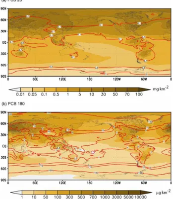
Figure 6 shows the simulation results of global atmospheric loadings (filled contours) of total PCB28 and 180 for spring of 2000 superimposed with the ratios (contour lines) of par-ticulate to gas phase PCBs. Both PCBs follow the global distributions of their respective emission patterns with obvi-ous inter-continental and polar transports while the absolute magnitude of atmospheric loading for PCB28 is much larger than that of PCB180. It can be seen from the plots that the impact of aerosols on the PCB global distribution becomes significant for heavier PCBs such as 180. The ratio ranges around 0.1 for the volatile PCB28 and reaches as high as 100 for PCB180.
Fig. 6. Column loadings of the total atmospheric PCB28 and PCB180 (filled contours) and ratios of particulate to gaseous PCB28 and PCB180 (contour lines) in the atmosphere for spring of 2000.
their high vapour pressures, lighter PCBs (e.g. 28) are mostly found in the atmosphere without attaching to any particles. The transport and deposition processes are governed by the principles of gaseous molecules, which makes them easily engaged in long range transport. On the contrary, semi-volatile PCBs are partitioned between atmosphere and par-ticulates depending on the physicochemical properties of the PCBs and the environmental conditions. The dry and wet de-positions of these particle-bound PCBs are much larger than those of gaseous phase PCBs. Consequently, heavier PCBs deposit back to the ground close to the source regions. The portion that engages in the long range transport is largely as-sociated with particulate matters. For PCB180, the ratio of particulate to gaseous loading for spring varies from around 1.0 between 0◦–30◦N, to around 10 between 30◦–60◦N and
to around 100 between 60◦
–90◦
N, reflecting the impact of temperature on the partitioning of PCB180 to the aerosol par-ticles. The seasonal variations of the ratios also reflect the impact of temperatures with smaller portions in the particu-late phase in boreal summers than in winters.
Observations have also shown the similar behaviours of PCBs. For IADN stations where particle and gas phase PCBs were analyzed separately in 1995 using high-volume sam-plers, the ratios in winter and summer are 0.02 and 0.32 for PCB28, and 0.06 and 4.17 for PCB180 (Table 3). It is noted that these ratios were measured under surface
con-Table 3.Ratios of particulate to gaseous PCBs at three IADN sta-tions.
Locations Season Month PCB28 PCB180
BBD Sleeping Bear Dunes
Winter DJF 0.3224 4.1782 Spring MAM 0.0570 0.2240 Summer JJA 0.0963 0.0785
Fall SON 0.0568 0.0423
EGH Eagle Harbor
Winter DJF 0.1817 0.7596 Spring MAM 0.1034 0.2802 Summer JJA 0.0581 0.1835
Fall SON 0.0523 0.0154
STP Sturgeon Point
Winter DJF 0.1730 1.1782 Spring MAM 0.0439 0.5043 Summer JJA 0.0200 0.0695
Fall SON 0.0330 0.1220
ditions while the model predictions were for the entire at-mospheric column loadings where colder environments aloft favoured more partitioning of PCBs to the particulate phases. It is usually very difficult to accurately determine the ratios of particulate to gaseous phase PCBs. Mandalakis et al. (2002) pointed out that high amounts of PCBs may volatilize from fine particles during aerosols sampling using conventional high-volume samplers and found that average volatilization losses, determined by the diffusion denuder system, varied between 54 and 97%, showing a strong dependence on par-tial pressure of individual PCB congeners and air temper-ature. Compared with IADN particulate fraction of PCBs (Table 3), GEM/POPs modeling results agreed with the gen-eral trends but over-estimated the ratios, which is consistent with the shortcoming for measuring particulate PCBs using high-volume samplers.
5 Conclusions
It is found that lighter PCB congeners are more volatile, less partitioned to particle phase and reach higher concen-trations in the air column. They can be readily transported long distances on the prevailing air currents and may remain in the atmosphere for a long period of time. Heavier PCBs are predicted to be relatively involatile, existing mainly in the particle-phase, and partitioning back to the surface at colder temperatures. The ratio of particle-phase to gas-phase PCB 28 is less than 0.1 while the ratio for PCB 180 ranges from 1.0 to 100 inversely proportional to temperatures.
CAN/POPs has been developed to study the behaviours of semi-volatile POPs in the atmosphere and the initial evalu-ation suggested that the model can reasonably simulate the transport and deposition of various PCBs. This lays the foundation for the assessment of the global cycles of vari-ous PCBs beginning with a companion paper on their inter-continental transport, deposition and budgets. Subsequent investigation of other POPs such as DDTs in the atmosphere will follow.
Acknowledgement. The authors wish to thank CFCAS (The
Canadian Foundation for Climate and Atmospheric Sciences) for its partial finical support for this research through the NW AQ MAQNet Grant and T. Harner and M. Shoeib for their work in analyzing PCBs in Chinese soil samples. The authors also wish to thank S. Venkatesh for his careful reading of this manuscript and valuable suggestions.
Edited by: W. E. Asher
References
Achman, D. R., Hornbuckle, K. C., and Eisenreich, S. J.: Volatiliza-tion of Polychlorinated Biphenyls from Green Bay, Lake Michi-gan, Environ. Sci. Technol., 27, 75–87, 1993.
Anderson, P. N. and Hites, R. A.: OH Radical Reactions: The Major Removal Pathway for Polychlorinated Biphenyls from the Atmo-sphere, Environ. Sci. Technol., 30, 1756–1763, 1996.
Atkinson, R. and Aschmann, S. M.: Rate Constants for the Gas-Phase Reaction of Hydroxyl Radicals with Biphenyl and the Monochlorobiphenyls at 295K, Environ. Sci. Technol., 19, 462– 464, 1985.
Bidleman, T. F., Falconer, R. L., and Harner, T. (Eds.): Parti-cle/Gas Distribution of Semivolatile Organic Compounds: Field and Laboratory Experiments with Filtration Samplers. Gas and Particle Partition Measurements of Atmospheric Organic Com-pounds, Gordon and Breach Publishers, Newark, New Jersey, 1998.
Breivik, K., Sweetman, A., Pacyna, J. M., and Jones, K. C.: To-wards a global historical emission inventory for selected PCB congeners – a mass balance approach 1. Global production and consumption, Sci. Total Environ., 290, 181–198, 2002a. Breivik, K., Sweetman, A., Pacyna, J. M., and Jones, K. C.:
To-wards a global historical emission inventory for selected PCB congeners - a mass balance approach 2. Emissions, Sci. Total Environ., 290, 199–224, 2002b.
Cˆot´e, J., Gravel, S., M´ethot, A., Patoine, A., Roch, M., and Stan-iforth, A.: The operational CMC-MRB Global Environmental
Multiscale (GEM) model: Part I – Design considerations and formulation, Mon. Wea. Rev., 126, 1373–1395, 1998.
de Cuevas, B. A., Webb, D. J., Coward, A. C., Richmond, C. S., and Rourke, E.: The UK Ocean Circulation and Advanced Modelling Project (OCCAM), in: High Performance Computing, Proceed-ings of HPCI Conference 1998, edited by: Allan, R. J., Guest, M. F., Simpson, A. D., Henty, D. S., and Nicole, D. A.,Plenum Press, Manchester, 325–335, 1999.
Falconer, R. L., Bidleman, T. F., and Cotham, W. E.: Preferential Sorption of Non-and-Mono-ortho-polychlorinated Biphenyls to Urban Aerosols, Environ. Sci. Technol., 29, 1666–1673, 1995. Finizio, A., Mackay, D., Bidleman, T., and Harner, T.: Octanol-air
partition coefficient as a predictor of partitioning of semi-volatile organic chemicals to aerosols, Atmos. Environ., 31, 2289–2296, 1997.
Foujols, M.-A., Levy, M., Aumont, O. and Madec, G.: OPA8.1 Tracer reference manual, Institut Pierre-Simon Laplace, 2000. Gong, S. L., Barrie, L. A., Blanchet, J.-P., Salzen, K. v., Lohmann,
U., Lesins, G., Spacek, L., Zhang, L. M., Girard, E., Lin, H., Leaitch, R., Leighton, H., Chylek, P., and Huang, P.: Canadian Aerosol Module: A size-segregated simulation of at-mospheric aerosol processes for climate and air quality mod-els 1. Module development, J. Geophys. Res., 108, 4007, doi:10.1029/2001JD002002, 2003.
Gusev, A., Mantseva, E., Shatalov, V., and Strukov, B.: Regional Multicompartment Model MSCE-POP, EMEP/MSC-E Techni-cal Report 5/2005, Moscow, 2005..
Halsall, C. J.: Investigating the occurence of pesistent organic pol-lutants (POPs) in the Arctic: Their atmospheric behaviour and interaction with the seasonal snow pack, Env. Poll., 128, 163– 175, 2004.
Hansen, K. M., Christensen, J. H., Brandt, J., Frohn, L. M., and Geels, C.: Modelling atmospheric transport persistent organic pollutants in Northern Hemisphere with a 3-D dynamical model: DEHM-POP, Atmos. Chem. Phys., 4, 1125–1137, 2004, http://www.atmos-chem-phys.net/4/1125/2004/.
Harner, T. and Bidleman, T. F.: Measurement of Octanol-Air Par-tition Coefficients for Polychlorinated Biphenyls, J. Chem. Eng. Data, 41, 895–899, 1996.
Harner, T. and Bidleman, T. F.: Octanol-Air Partition Coefficient for Describing Particle/Gas Partitioning of Aromatic Compounds in Urban Air, Environ. Sci. Technol., 32, 1494–1502, 1998. Harner, T., Pozo, K., Gouin, T., Macdonald, A.-M., Hung, H.,
Cainey, J., and Peters, A.: Global pilot study for persistent or-ganic pollutants (POPs) using PUF disk passive air samplers, En-viron. Poll., 144, 445–452 2006.
Huang, P., Gong, S. L., Zhao, T. L., Neary, L., and Barrie, L. A.: GEM/POPs: a global 3-D dynamic model for semi-volatile per-sistent organic pollutants – Part 2: Global transports and budgets of PCBs, Atmos. Chem. Phys., 7, 4015–4025, 2007,
http://www.atmos-chem-phys.net/7/4015/2007/.
and Rosenberg, B.: Temporal trends of organochlorine pesticides in the Canadian Arctic atmosphere, Env. Sci. Technol., 36, 862– 868, 2002.
Hung, H., Lee, S. C., Wania, F., Blanchard, P., and Brice, K.: Mea-suring and simulating atmospheric concentration trends of poly-chlorinated biphenyls in the Northern Hemisphere, Atmos. Env-iron., 39, 6502–6512, 2005b.
Junge, C. E. (Ed.): Fate of Pollutants in the Air and Water Environ-ments, 1. J. Wiley, New York, 7–26, 1977.
Jury, W. A.: Volatilization From soil, in:Vadose Zone Modeling of Organic Pollutants, 3rd ed., edited by: Hern, S. C. and Melancon, S. M., Lewis Publishers Inc., Michigan, 1989.
Jury, W. A., Spencer, W. F., and Farmer, W. J.: Behavior Assess-ment Model for Trace Organics in Soil: I.Model Description, J. Environ. Qual., 12, 558–564, 1983.
Karickhoff, S. W.: Semi-Empirical Estimation of Sorption of Hy-drophobic Pollutants on Natural Sediments and Soils, Chemo-sphere, 10, 833–846, 1981.
Koziol, A. S. and Pudykiewicz, J. A.: Global-scale environmen-tal transport of persistent organic pollutants, Chemosphere, 45, 1181–1200, 2001.
Kwok, E. S. C., Atkinson, R., and Arey, J.: Rate Constants for the Gas Phase Reactions of the OH Radical with Dichloro-biphenyls, 1-Chlorodibenzo-p-dioxin, 1,2-Dimethoxybenzene, and Diphenyl Ether: Estimation of OH Radical Reaction Rate Constants for PCBs, PCDDs, and PCDFs, Environ. Sci. Tech-nol., 29, 1591–1598, 1995.
Li, Y.-F.: Global Population Distribution Database, A Report to the United Nations Environment Programme, under UNEP Sub-Project FP/1205-95-12, 1996.
Liss, P. S. and Slater, P. G.: Flux of Gases across the Air-Sea Inter-face, Nature, 247, 181–197, 1974.
Ma, J., Daggupaty, S., Harner, T., and Li, Y.-F.: Impacts of Lindane usage in the Canadian prairies on the Great Lakes ecosystem, 1. Coupled atmospheric transport model and modeled concen-trations in air and soil, Environ. Sci. Technol., 37, 3774–3781, 2003.
Mackay, D.: Multimedia Environmental Models, The Fugacity Ap-proach, Lewis Publishers, 1991.
Mackay, D., Shiu, W. Y., and Ma, K. C.: Illustrated Handbook of Physical-Chemical Properties and Environmental Fate for Or-ganic Chemicals, I. Lewis Publishers Inc., Michigan, 1992. MacLeod, M., Woodfine, D., Mackay, D., McKone, T., Bennett, D.,
and Maddalena, R.: BETR North America: A Regionally Seg-mented Multimedia Contaminant Fate Model for North America, Environ. Sci. Pollut. Res., 8, 156–163, 2001.
Malanichev, A., Mantseva, E., Shatalov, V., Strukov, B., and Vu-lykh, N.: Numerical evaluation of the PCB transport over the Northern Hemisphere, Environ. Poll., 128, 279–289, 2004. Mandalakis, M. and Stephanou, E. G.: Polychlorinated biphenyls
associated with fine particles (pm2.5) in the urban environment of Chile: concentration levels, and sampling volatilization losses, Environ. Toxicol. Chem., 21, 2270–2275, 2002.
Meijer, S. N., Ockenden, W. A., Sweetman, A. J., Breivik, K., Gri-malt, J. O. and Jones, K. C.: Global distribution and budget of PCBs and HCB in background surface soils: implications for sources and environmental processes, Environ. Sci. Technol., 37, 667–672, 2003.
Pankow, J. F.: Review and Comparative Analysis of the Theories on Partitioning Between the Gas and Aerosol Particulate Phases in the Atmosphere, Atmos. Environ., 21, 2275–2283, 1987. Sahsuvar, L.: Modelling Physical Chemical Properties and
Path-ways of Polychlorinated Biphenyls in the Atmosphere, MSc The-sis, York University, Toronto, 140 pp., 1999.
Sahsuvar, L., Helm, P. A., Jantunen, L. M., and Bidleman, T. F.: Henry’s law constants for alpha-, beta-, and gamma-hexachlorocyclohexanes (HCHs) as a function of temperature and revised estimates of gas exchange in Arctic regions, Atmos. Environ., 37, 983–992, 2003.
Schnoor, J. L.: Environmental Modeling. Fate and Transport of Pol-lutants in Water, Air, and Soil, Environmental Science and Tech-nology, John Wiley & Sons, Inc., New York, 1996.
Semeena, V. S., Feichter, J., and Lammel, G.: Impact of the regional climate and substance properties on the fate and atmospheric long-range transport of persistent organic pollutants – exampled of DDT andγ-HCH, Atmos. Chem. Phys., 6, 1231–1248, 2006, http://www.atmos-chem-phys.net/6/1231/2006/.
Semeena, V. S. and Lammel, G.: The significance of the grasshopper effect on the atmospheric distribution of presi-dent organic substances, Geophys. Res. Lett., 32, L07804, doi:10.1029/2004GL022229, 2005.
Shen, L., Wania, F., Lei, Y. D., Teixeira, C., Muir, D. C. G., and Xiao, H.: Polychlorinated biphenyls and polybrominated diphenyl ethers in the North American atmosphere, Environ. Poll., 144, 434–444, 2006.
Sobek, A. and Gustafsson, O.: Latitudinal fractionation of poly-chlorinated biphenyls in surface seawater along a 62 degrees N-89 degrees N transect from the southern Norwegian Sea to the North Pole area, Environ. Sci. Technol., 38, 2746–2751, 2004. Strand, A. and Hov, Ø.: A model strategy for the simulation of
chlorinated hydrocarbon distributions in the global environment, Water Air Soil Poll., 86, 283–316, 1996.
Sun, P., Backus, S., Blanchard, P., and Hites, R. A.: Annual vari-ation of polycyclic aromatic hydrocarbon concentrvari-ations in pre-cipitation collected near the Great Lakes, Environ. Sci. Technol., 40, 696–701, 2006.
Toose, L., Woodfine, D. G., MacLeod, M., Mackay, D., and Gouin, J.: BETR-World: a geographically explicit model of chemical fate: application to transport of alpha-HCH to the Arctic, Envi-ron. Poll., 128, 223–240, 2004.
van Jaarsveld, J. A., van Pul, W. A. J., and de Leeuw, F. A. A. M.: Modelling transport and deposition of persistent organic pollu-tants in the European region, Atmos. Env., 31, 1011–1024, 1997. Venkatram, A., Karamchandani, P. K., and Misra, P. K.: Testing a comprehensive acid deposition model, Atmos. Environ., 22, 737–747, 1988.
Wania, F. and Daly, G. L.: Estimating the contribution of degrada-tion in air and deposidegrada-tion to the deep sea to the global loss of PCBs, Atmos. Environ., 36, 5581–5593, 2002.