© European Geosciences Union 2003
and Earth
System Sciences
Slope stability monitoring from microseismic field using polarization
methodology
Yu. I. Kolesnikov, M. M. Nemirovich-Danchenko, S. V. Goldin, and V. S. Seleznev Institute of Geophysics SB RAS, 3 Pr. Akademika Koptyuga, 630090 Novosibirsk, Russia Received: 7 October 2002 – Revised: 6 January 2003 – Accepted: 7 January 2003
Abstract.Numerical simulation of seismoacoustic emission (SAE) associated with fracturing in zones of shear stress con-centration shows that SAE signals are polarized along the stress direction. The proposed polarization methodology for monitoring of slope stability makes use of three-component recording of the microseismic field on a slope in order to pick the signals of slope processes by filtering and polarization analysis. Slope activity is indicated by rather strong roughly horizontal polarization of the respective portion of the field in the direction of slope dip. The methodology was tested in microseismic observations on a landslide slope in the North-ern Tien-Shan (Kyrgyzstan).
1 Introduction
Reliable assessment of slope stability, especially important in urban regions, helps to assure human safety, to cut down the costs and evaluate the efficiency of landslide mitigation, and to reduce economic losses from catastrophic landslides. Slope failure occurs when tangential stress overcomes the shear strength of rocks, and a rock mass detached from the slope moves downhill along a slip surface. The formation of a sliding surface is preceded by more or less long stress concentration in its vicinity associated with numerous micro-and medium-scale changes to strained rocks.
These changes include forming and healing of cracks ac-companied by release of microseismic energy (called acous-tic or seismoacousacous-tic emission), which was observed in many experiments (Goodman and Blake, 1965; Cadman and Good-man, 1967; Postoev, 1972; Rouse et al., 1991). Seismoacous-tic emission makes up a great portion of the microseismic field on active slopes, and its parameters (intensity, energy, and spectral patterns) have been broadly used in landslide monitoring (McCauley, 1976; Muravin et al., 1987; Muravin et al., 1991; Adushkin et al., 1993; Dixon et al., 1996).
Correspondence to:Yu. I. Kolesnikov ([email protected])
Cracks that arise in the vicinity of a forming sliding sur-face often have preferred orientations produced by stresses in rocks, and polarization analysis appears a useful tool in studies of microseismic fields in landslide sites. First appli-cations of this approach were reported by Zyatev et al. (1998) who revealed strongly differing polarization patterns of mi-croseisms on active and inactive parts of slopes during land-slide studies near Tomsk (West Siberia, Russia).
In this paper we apply numerical simulation to analyze the polarization of microseismic signals relevant to landslide hazard. The modeling results provided a basis for the po-larization methodology to be used in slope stability monitor-ing from microseismic field. The methodology was tested during processing and interpretation of field data from three-component microseismic observations on a landslide slope in the Suusamyr valley in the Northern Tien-Shan, Kyrgyzstan.
2 Numerical simulation of seismoacoustic emission from a forming sliding surface
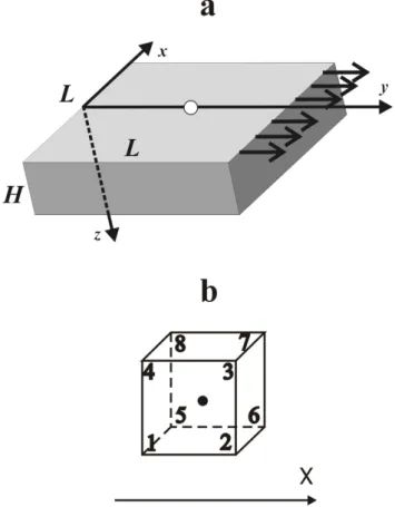
A landslide was modeled as a homogeneous isotropic paral-lelepiped with a square base (Fig. 1a). Its upper bound (the planeZ = 0) is uniformly and constantly loaded along the Y-axis and the sides are free from loading. For the sake of computation, the study domain is represented as a grid of cu-bic elementary cells.
The bottom bound simulates the forming sliding surface. The weak zone is modeled under the assumption that at a zero time a half of the cells on the bottom bound can slide freely, without friction, along theY-axis, and the other cells remain fixed in randomly set coordinates. This boundary condition, together with the conditions on the upper bound, provides stress concentration on the bottom bound.
Fig. 1.Geometry of numerical model(a)and elementary cubic cell of computational grid(b).
is solved in a dynamic formulation with variable boundary conditions on the boundZ=H. The calculations are made using the first Cauchy’s law (motion equations in stresses)
∂σij ∂ζj =
ρu¨i
and the defining stress-strain relations as the incremental Hooke’s law (Germain, 1962)
σij∇=cij klε˙kl, where
σij∇= dσij
dt −ikσkj −j kσki
is Jaumann’s derivative,σij andεijare stress and strain ten-sor components, respectively, ij are spin tensor compo-nents,ρis density,uiare components of displacement vector, cij kl are components of fourth-order tensor of elastic con-stants,t is time, andζi are Cartesian coordinatesX,Y, and Z.
Displacements and particle velocities are found in the nodes of the cubic cells, and strain velocities are calculated from displacement velocities in their centers:
˙
εij = 1 2
∂
˙
ui ∂ζj +
∂u˙j ∂ζi
.
Fig. 2. Computed displacement velocities (vectors) for the central part of the model. Arrows show direction of load applied to upper bound.
Spatial derivatives are obtained by averaging over the re-spective bounds of the cubic cells, e.g. for theζ11component it is (indexing of nodes is in Fig. 1b)
˙
ε11= 1 41ζ
(u˙1)2+(u˙1)3+
(u˙1)6+(u˙1)7−(u˙1)1−(u˙1)4−(u˙1)5−(u˙1)8
, (1)
where1ζ is side of cells.
Other components are determined in the same way. For details of the method see Nemirovich-Danchenko (1998). The method allows simulation of SAE signals associated with the formation of a sliding surface. The modeling pa-rameters we used wereH = 20 m for the thickness of the parallelepiped, L = 200 m for the length and width of its base, P-wave velocity VP = 1000 m/s, S-wave velocity VS = 500 m/s, density ρ = 2200 kg/m3, and a 0.5 m grid (side of cells).
The modeling shows that loading applied to the upper bound causes stress concentration on the bottom bound. A shear crack arises when the critical stress is achieved in any computation cell. The forming of shear cracks, in turn, re-leases elastic energy producing sources of seismic waves dis-tributed randomly over the model base.
Figure 2 shows a computed vectorial wave pattern for the central part of the model (40×40×20 m3) for the doubled traveltime of a direct wave from the earliest triggered source, i.e. the effect of the lateral model boundaries is excluded. SAE signals from several events are clearly seen in the fig-ure, which is actually a numerical snapshot of the vector field of displacement velocities. The maximum-amplitude vectors on the upper bound of the model for each event roughly fol-low the direction of the load applied to this bound.
a
b
X
Y
Y
Z
Fig. 3.Computed projections of particle trajectories on planesZ=
0(a)andX=0(b).
Note that the trajectory shown in Fig. 3 is a stack of signals from several sources in different points of the model’s lower bound, i.e. the direction of predominant polarization on the surface depends rather on the direction of shear stress than on the position of the sources. Applied to slope processes (on relatively shallow slopes), this is a roughly horizontal po-larization of a certain portion of the microseismic field along the slope dip. Isolated from the total field, this portion may be diagnostic of slope activity.
3 Field microseismic observations on a landslide slope
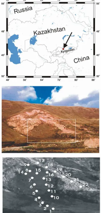
The polarization methodology was tested during processing of field data from microseismic observations on a landslide slope in the Suusamyr valley (Northern Tien-Shan, Kyrgyzs-tan). The landslide (Fig. 4), 250–300 m in width and in length, was produced by theM=7.3 Suusamyr earthquake of August 1992 at an altitude of 2400 m. The displaced rocks are up to 50–70 m thick and estimates of their volume are from 0.5 to 1.0×10⁶m3(Havenith et al., 2000). The slope in this site is about 30◦steep and dips towards an azimuth of 140−160◦. It is composed of Quaternary sands and clays lying upon consolidated clays and includes bedrock blocks. In its lower part the landslide splits into three lobes (each a few hundreds of meters long) separated by unbroken parts of the slope.
The latter are also potentially hazardous as they are cut with numerous surface cracks, up to tens of centimeters wide. Some of them are accompanied by micro-landslides. The microseismic field in various parts of the slope (Fig. 4c) was monitored by a portable four-channel digital station based on a laptop computer. The instrument, including a battery, cables, a three-component geophone, and pre-amplifiers, is mounted on a small two-wheel carriage easy to draw even in the mountains.
The instrument has a broad frequency band from 10 Hz to 100 kHz with programmable digitization frequency from 2 kHz to 1 MHz. The broadband recording was used, as we had noa prioriinformation on the frequency content of the microseismic field in this region. According to published data (Muravin et al., 1991), the frequency of SAE signals
Fig. 4. (a)Location map of Kyrgyzstan (landslide site is shown by arrow). (b)Landslide slope and monitoring area (within the box).
(c)Instrument layout.
recorded on slopes prone to landsliding may vary from a few hertz to hundreds of kilohertz in function of slope geology.
0 50 100 150 200 250
frequency, Hz 0
1
0,2 0,4 0,6 0,8
normalized relative amplitude
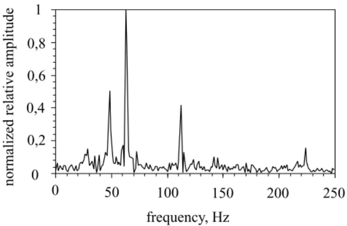
Fig. 5.Spectrum of a non-filtered microseismic signal.
component). At each measurement point five 0.6 s time se-ries were acquired and digitized at a step of 0.1 ms.
4 Processing and analysis of microseismic data
The observations were run in noisy conditions because of roadwork in the vicinity of the landslide, which required a preliminary spectral analysis of the records. The spectra of most traces contained typically cultural quasi-harmonic noise in the 50–120 Hz bandwidth and above 210 Hz, stand-ing out as narrow peaks about 50, 65, 110, and 225 Hz (Fig. 5). Therefore, we applied 10–45 and 120–210 Hz band-pass filtering and used two sets of filtered data in the further processing.
The next step implied visualization of the projections of particle motion onto horizontal and vertical planes. The po-larization of the projections showed no regularity in the broad band (prior to filtering, Fig. 6a) and at low frequencies (10– 45 Hz, Fig. 6b), but a well-defined polarization was observed in the high-frequency bandwidth (120–210 Hz, Fig. 6c). Po-larization had about the same direction as the slope dip, ex-cept for few weakly polarized responses on a terrace beneath the slope, on rocks over large cracks, and on the surface of rocks deformed by the landslide, i.e. in unloaded points.
The polarization patterns at different frequencies may be explained as follows. The low-frequency signals, which make up the greatest portion of the broadband (non-filtered) response, come from remote sources outside the landslide slope and thus have no preferred orientations.
The signals from remote high-frequency sources, which are as a rule weaker than the low-frequency ones, almost elude recording because of spreading and attenuation. There-fore, polarization of high-frequency noise may be associated with the forming of micro-cracks in rocks, which is implic-itly confirmed by the orientation of the principal polarization axis along the slope dip.
Then we determined the numerical parameters of polariza-tion by more detailed processing of the horizontal and verti-cal projections of particle motion from the high-frequency
N
S
Fig. 6. Horizontal projections of particle trajectories in a point on slope, from records before(a)and after 10–45 Hz (b) and 120– 210 Hz(c)bandpass filtering.
portion of the microseismic field, using five 0.6 s three-component records from each point.
The seismic tracesxi,yi,zi(i=1, ...,N) recorded by the three-component geophone with its sensors oriented along the coordinatesX,Y,Z, were considered as sets of the re-spective coordinates of the geophone subject to discrete vari-ations with time under the effect of microseisms. We applied least-square approximation by a straight liney =ax to the points (xi, yi) on the horizontal plane Z = 0, where a is given by
a1,2= −
b±√b2+4c2
where
b= N X
i=1
xi2−yi2,
c= N X
i=1 xiyi.
Then standard deviationsσ1andσ2of the points (xi,yi) from the linesy =a1x andy = a2x (one approximating the set of points and the other positioned perpendicular to it) were found as
σ1= v u u u t N P i=1
(xisinα1−yicosα1)2
N ,
σ2= v u u u t N P i=1
(xisinα2−yicosα2)2
N ,
where
α1=tan−1a1, α2=tan−1a2.
Finally, the polarization factor in the horizontal plane was expressed through the parameterPhcalculated from the stan-dard deviationsσ1andσ2as
Ph=1−
min(σ1, σ2) max(σ1, σ2)
, (0≤Ph≤1).
The parameterPhis a numerical expression of polarization in some direction within the planeZ = 0. The direction is defined by a straight line drawn through the origin of the coordinates at an angleαh(polarization angle) toX, which is eitherα1orα2, depending on which of the two corresponds to the least standard deviation of the points (xi,yi) from the respective straight liney =ax.
This line controls the position of the vertical plane, which was the subject of the further processing. The parameters of polarization in the vertical plane (polarization factorPvand angleαv) were found in the same way as for the horizontal plane, but the traceziwas used instead ofyi and the projec-tionξi onto the horizontal polarization direction instead of xi, whereξi is given by
ξi =xicosαh+yisinαh.
Thus, the polarization of high-frequency microseismic noise can be analyzed using four parameters – the polariza-tion factorsPhandPv, and the anglesαhandαv– that repre-sent polarization in a horizontal and a vertical planes, respec-tively (Table 1). Note that we limited ourselves to just one possible approach to polarization analysis. Similar results can be obtained from other algorithms, such as the covari-ance matrix approach (Flinn, 1965).
5 Discussion
Now we interpret the processed field data (Table 1) with re-gard to numerical modeling (Sect. 2). The modeling shows that SAE signals from the zone of maximum shear stress should polarize mostly along the stress direction. The polar-ization of the fracturing-related portion of the microseismic field on relatively shallow-dipping slopes is nearly horizontal and dip-parallel.
Of course, this polarization pattern may be distorted by refractions and reflections in the landslide body producing a complex velocity structure (e.g. numerous steep interfaces). However, earlier studies of the same slope by active seismic and electric techniques (Havenith et al., 2000) show a quite plain upper section.
We analyzed the polarization of particle motions caused by microseisms in the 120–210 Hz bandwidth (the bandwidth hypothesized to represent seismoacoustic emission associ-ated with fracturing in zones of stress concentration).
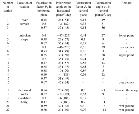
The signals from the river terrace (points 1–3) sloping at
≤ 10◦ show a weak horizontal polarization in a direction roughly parallel to the slope dip, with low polarization fac-tors. The factors of vertical polarization are also low, i.e. horizontal and vertical oscillations have comparable ampli-tudes. The weak polarization indicates that the SAE com-ponent is much below the microseisms from other sources (wind, water streams, or cultural noise, etc.), which allows us to assume that the slope within the terrace is inactive. The records on the surface of rocks deformed by landsliding (points 17–22) have small vertical components, i.e. show a nearly horizontal polarization. Polarization in the horizontal plane is rather weak in three points in the middle of the pro-file (points 18–20) but very strong in the upper and two lower points, where the oscillations are polarized roughly along the slope dip. This part of the landslide is U-shaped following a small gully made by a creek originated from a groundwa-ter spring in the upper point of the profile, along the central lobe, and this polarization pattern may have been produced by effects of secondary slopes.
In the lower part of the profile (points 21–22) the surface flattens as the lobe reaches the river terrace, and the slope is much less dissected. The ground is wetter there because of poor consolidation and infiltration from the creek running downhill (the infiltration is implicitly indicated by small wa-ter basins in the creek vicinity). The wawa-ter-saturated ground loses its strength, which may increase polarization in this part of the profile. The uppermost point on the lobe (point 17) also shows a strong polarization apparently associated with additional loading as∼20 m uphill from the station the slope abruptly becomes much steeper making a 10 m high scarp.
Table 1.Parameters of polarization of microseismic field on landslide slope within 120–210 Hz bandwidth
Number Location of Polarization Polarization Polarization Polarization Remark of station factorPhin angleαhin factorPvin angleαvin
station horizontal horizontal vertical vertical plane planea, deg plane planceb, deg
1 river 0,45 26 (154) 0,13 49 –
2 terrace 0,5 −2 (182) 0,38 81 –
3 0,37 37 (143) 0,14 36 –
4 unbroken 0,4 −47 (227) 0,44 27 lower point
5 slope 0,78 23 (157) 0,7 9 –
6 0,67 36 (144) 0,75 6 –
7 0,3 −46 (226) 0,51 29 over a crack
8 0,73 31 (149) 0,81 3 –
9 0,55 30 (150) 0,37 28 upper point
10 0,7 35 (145) 0,74 4 –
11 0,47 23 (157) 0,56 13 –
12 0,65 33 (147) 0,65 7 –
13 0,88 10 (170) 0,89 3 –
14 0,69 −1 (181) 0,56 22 –
15 0,77 31 (149) – – –
16 0,07 46 (134) – – over a crack
17 deformed 0,84 20 (160) 0,5 −4 beneath the scarp
18 rocks 0,32 −11 (191) 0,63 9 –
19 (landslide 0,3 −6 (186) 0,35 −8 –
20 body) 0,17 −3 (183) 0,7 −1 –
21 0,59 32 (148) 0,41 −8 wet ground
22 0,66 20 (160) 0,79 −12 wet ground
aCounter-clockwise from southward direction. Numbers in parentheses are angles expressed as azimuth (dip azimuth of slope in monitoring site is about 140−160◦).
bAngles relative to the horizontal plane, positive upward and negative downward facing the terrace.
polarization is weak or absent over large cracks (points 7 and 16), i.e. in points of unloading.
Polarization is also weak in the lower part of the unbro-ken slope (point 4) where the ground is naturally confined by the terrace below, and in its uppermost part (point 9) above which the slope abruptly becomes much lower-angle. In gen-eral, the observed relatively strong polarization of the high-frequency portion of the microseismic response from unbro-ken parts of the slope may indicate potential landslide haz-ard. Landslide may be triggered by seismic or hydrological and meteorological effects.
6 Conclusions
The numerical simulation showed that fracturing in zones of shear stress concentration may cause polarization of SAE signals along the stress direction. This property of the SAE portion of the microseismic field made the basis of the pro-posed polarization methodology applicable to the monitor-ing of slope stability. The method implies passive three-component recording of the microseismic field on a slope and picking its portion related to slope processes by filtering and
polarization analysis. The activity of the slope is indicated by strong horizontal polarization parallel to the slope dip in the proper frequency components. This methodology was proven to be efficient during processing of field data from a landslide site in the Northern Tien-Shan and can be suc-cessfully used, along with other methods, for slope stability monitoring in regions of landslide hazard.
Acknowledgements. The study was supported by grants IC15-CT97-0202 (EC, DG XII) from the European Community and 00-05-65337 from the Russian Foundation for Basic Research. We thank A. D. Duchkov, A. F. Emanov, and T. A. Charimov for orga-nization and S. V. Polozov and G. V. Larkin for logistic support of the field experiments. The paper profited much from the construc-tive criticism of two anonymous reviewers.
References
Adushkin, V. V., Spivak, A. A., Bashilov, I. P., Spungin, V. G., Du-binya, V. A., and Ferapontova, E. N.: Relaxation monitoring in the Southern Alps on unstable mountain slopes, Izv. AN SSSR, Ser. Fizika Zemli, (in Russian), 10, 103–107, 1993.
Dixon, N., Kavanagh, J., and Hill, R.: Monitoring landslide activity and hazard by acoustic emission, J. Geol. Soc. China, 39, 4, 437– 484, 1996.
Flinn, E. A.: Signal analysis using rectilinearity and direction of particle motion, Proc. IEEE, 53, 12, 1874–1876, 1965.
Germain, P.: M´ecanique des milieux continus, Paris, 1962. Goodman, R. and Blake, W.: An investigation of rock noise in
land-slides and cut slopes, Rock Mechanics and Engineering Geology, 2, 88–93, 1965.
Havenith, H.-B., Jongmans, D., Abdrakhmatov, K., Trefois, P., Del-vaux, D., and Torgoev, I. A.: Geophysical investigations of seis-mically induced surface effects: case study of a landslide in the Suusamyr Valley, Kyrgyzstan, Surv. Geophys., 21, 4, 349–369, 2000.
McCauley, M. L.: Microseismic detection of landslides, In: Innova-tion in Subsurface ExploraInnova-tion of Soil, NaInnova-tional Research Coun-cil (National Academy of Sciences), Transport Research Board, 581, 25–30, 1976.
Muravin, G. B., Erminson, A. L., and Sigalovsky M. N.: A system
for investigation of ground motion by acoustic emission, Defek-toskopia, (in Russian), 3, 62–66, 1987.
Muravin, G. B., Sigalovsky M. N., Rozumovich, E. E., and Lezvin-skaya L. M.: Acoustic emission applied to ground motion studies (An overview), Defektoskopia, (in Russian), 11, 3–17, 1991. Nemirovich-Danchenko, M. M.: A model for the brittle
hypoelas-tic medium: the application to computation of deformations and failure in rock, Physical Mesomechanics, 2, 101–108, 1998. Postoev, G. P.: Some results of seismoacoustic monitoring in a
land-slide site in the Zeravshan valley, Bull. VSEGINGEO, (in Rus-sian), Moscow, 56, 65–71, 1972.
Rouse, C., Styles, P., and Wilson, S. A.: Microseismic emissions from flowslide-type movements in South Wales, Eng. Geol., 31, 1, 91–110, 1991.