A NEW APPROACH FOR MODELING AND CONTROL OF NONLINEAR
SYSTEMS VIA NORM-BOUNDED LINEAR DIFFERENTIAL INCLUSIONS
Roman Kuiava
∗Rodrigo A. Ramos
†Hemanshu R. Pota
‡∗Federal University of Parana (UFPR), Polytechnic Center, Department of Electrical Engineering, Rua Cel. Francisco
Heraclito dos Santos, 100, Jardim das Americas, 81531-980, Curitiba, Brazil
†University of Sao Paulo (USP), Engineering School of Sao Carlos (EESC), Department of Electrical Engineering, Av.
Trabalhador Saocarlense, 400, Centro, 13566-590, Sao Carlos, Brazil
‡University of New South Wales at Australian Defence Force Academy (UNSW@ADFA), School of Information
Technology and Electrical Engineering, Northcott Drive, Canberra, Australia
RESUMO
Uma nova abordagem para modelagem e controle de sis-temas n˜ao-lineares via inclus˜oes diferenciais lineares li-mitadas por norma
Este artigo prop˜oe um m´etodo sistematico para modelagem de sistemas n˜ao-lineares na forma de inclus˜oes diferenciais limitadas por norma (IDLNs). O modelo de IDLN resul-tante ´e adequado para aplicac¸˜ao de t´ecnicas de projeto de controle linear, o que possibilita atender crit´erios espec´ıficos de desempenho dinˆamico para o sistema n˜ao linear origi-nal em uma regi˜ao de operac¸˜ao de interesse no espac¸o de estados, a partir de um controlador linear projetado para a sua representac¸˜ao na forma de IDLN. Ent˜ao, um proce-dimento para projeto de um controlador por realimentac¸˜ao dinˆamica de sa´ıda para um sistema descrito na forma de IDLN ´e tamb´em proposto neste artigo. Uma das principais contribuic¸˜oes da abordagem proposta de modelagem e con-trole ´e a aplicac¸˜ao do teorema do valor intermedi´ario para representar sistemas n˜ao-lineares na forma de um modelo li-near com parˆametros variantes no tempo, o qual ´e ent˜ao ma-peado em uma inclus˜ao diferencial linear polit´opica (IDLP).
Artigo submetido em 24/03/2011 (Id.: 1308) Revisado em 05/05/2011, 24/08/2011, 06/09/2011
Aceito sob recomendac¸ ˜ao do Editor Associado Prof. Daniel Coutinho
Para evitar o problema combinat´orio inerente aos modelos polit´opicos para sistemas de m´edio e grande porte, a IDLP ´e transformada em uma IDLN, e este processo ´e feito de tal forma que todas as trajet´orias do sistema n˜ao-linear origi-nal sejam tamb´em trajet´orias do modelo resultante de IDLN. Al´em do mais, ´e tamb´em poss´ıvel escolher uma estrutura particular para os parˆametros da IDLN de forma `a reduzir o conservadorismo na representac¸˜ao do sistema n˜ao-linear pelo modelo de IDLN, e esta caracter´ıstica ´e tamb´em uma impor-tante contribuic¸˜ao deste artigo. Quanto ao projeto do contro-lador, ele ´e formulado como um problema de busca por uma soluc¸˜ao que satisfac¸a um conjunto de restric¸˜oes escritas na forma de desigualdades matriciais bilineares (ou BMIs, do inglˆes bilinear matrix inequalities). Tal soluc¸˜ao ´e ent˜ao en-contrada usando-se um procedimento de separac¸˜ao em duas etapas que transforma o conjunto original de BMIs em um conjunto correspondente de desigualdades matriciais lineares (ou LMIs, do inglˆes linear matrix inequalities). Dois exem-plos num´ericos s˜ao apresentados para demonstrar a eficiˆencia da abordagem proposta.
ABSTRACT
A systematic approach to model nonlinear systems using norm-bounded linear differential inclusions (NLDIs) is pro-posed in this paper. The resulting NLDI model is suitable for the application of linear control design techniques and, there-fore, it is possible to fulfill certain specifications for the un-derlying nonlinear system, within an operating region of in-terest in the state-space, using a linear controller designed for this NLDI model. Hence, a procedure to design a dynamic output feedback controller for the NLDI model is also posed in this paper. One of the main contributions of the pro-posed modeling and control approach is the use of the mean-value theorem to represent the nonlinear system by a linear parameter-varying model, which is then mapped into a poly-topic linear differential inclusion (PLDI) within the region of interest. To avoid the combinatorial problem that is inherent of polytopic models for medium- and large-sized systems, the PLDI is transformed into an NLDI, and the whole process is carried out ensuring that all trajectories of the underlying nonlinear system are also trajectories of the resulting NLDI within the operating region of interest. Furthermore, it is also possible to choose a particular structure for the NLDI pa-rameters to reduce the conservatism in the representation of the nonlinear system by the NLDI model, and this feature is also one important contribution of this paper. Once the NLDI representation of the nonlinear system is obtained, the paper proposes the application of a linear control design method to this representation. The design is based on quadratic Lya-punov functions and formulated as search problem over a set of bilinear matrix inequalities (BMIs), which is solved using a two-step separation procedure that maps the BMIs into a set of corresponding linear matrix inequalities. Two numer-ical examples are given to demonstrate the effectiveness of the proposed approach.
KEYWORDS: nonlinear systems; linear dynamic output feedback control; linear differential inclusions; robust con-trol; linear matrix inequalities.
1
INTRODUCTION
Stability analysis and control synthesis for complex systems (such as, nonlinear systems involving saturation or time-varying uncertainties) can be simplified by the use of linear descriptions of these dynamical systems in the form of linear differential inclusions (LDIs). Generally speaking, it may be possible to ensure that the trajectories of such a system ex-hibit certain features by analyzing a corresponding model in the form of an LDI. Necessary conditions that guarantee, for example, the existence of a polytopic LDI (PLDI) containing all trajectories of a particular nonlinear system are discussed and demonstrated in (Boyd et al., 1994; Hu and Chen, 2007).
A wide variety of analysis and control problems have been formulated and solved for different classes of LDIs, most of them in the form of linear matrix inequalities (LMIs) (e.g., (Boyd et al., 1994); (Xie and de Souza, 1992; Bernard et al., 1997)). The LMI approach makes it easy to include stability and performance specifications (such as, a minimum decay rate and bounds on the output peak values) in the for-mulation of analysis and synthesis problems for LDIs. Once the problem is written in terms of LMIs, efficient convex search or optimization methods can be used to find a solu-tion to it (Boyd et al., 1994). Based on this feature, it may be easier to design a controller for a nonlinear system using a linear description of it in the form of an LDI.
The modeling, analysis and control of nonlinear systems via linear models are not restricted to approaches based on LDIs. In this sense, Mamdani and Takagi Sugeno fuzzy systems play also an important role (Montagner et al., 2010; Mozelli et al., 2010; Tognetti and Oliveira, 2010). These type of fuzzy systems allow nonlinear systems to be approximated by means of an averaged sum of linear models. Then, the problems of analysis and synthesis can be written in terms of LMIs (Montagner et al., 2010; Mozelli et al., 2010). Also, based on feedback linearization technique, adaptative neu-ral networks or fuzzy control schemes have been introduced to approximate nonlinear systems into linear models (Chen et al., 1996).
This paper addresses both modeling and control of nonlin-ear systems via a particular class of LDIs: the class of the norm-bounded LDIs (NLDIs). The main idea behind the modelling technique is to represent the nonlinear system by a linear parameter-varying (LPV) system using the mean value theorem (Vidyasagar, 1993; Zemouche et al., 2005; Hossain et al., 2009). This LPV system can be particularly repre-sented by a PLDI, provided that a certain set of conditions (that will be presented later in the paper) are satisfied.
It is possible to use LMIs to check the quadratic stability of a PLDI, but this requires the solution of one LMI for each of the vertices of the polytopic domain. One major drawback of this approach is the fact that, in general, the number of ver-tices of this polytope is high (see the numerical examples in (Hu and Chen, 2007; Hu, 2007)), and this translates into sig-nificant (and sometimes intractable) computational burden.
former is also a trajectory of the latter. The formulation pro-posed in (Boyd et al., 1994) is based on the solution of an LMI feasibility problem and considers only the case where a specific matrix parameter of the NLDI is square and in-vertible. This condition is substituted here by a weaker one in which this matrix parameter must only have full column rank (and this is another important contribution of this pa-per). Using this weaker condition, it is possible to choose a particular structure of the NLDI parameters in order to re-duce the conservatism in the representation of the underlying nonlinear system by the NLDI model.
Based on this approach for modeling a nonlinear system via an NLDI, this paper proposes the design of a linear dynamic output feedback (LDOF) controller for the NLDI model, in such a way that stability and performance speci-fications can be satisfied for the closed-loop nonlinear sys-tem using a linear controller. The motivation for focusing on this type of control comes from problems in the area of power systems stability (see, for example, (Basler and Schae-fer, 2008; Ramos et al., 2004; Hossain et al., 2009)), in which linear controllers are often applied to a system with highly nonlinear behaviors, and these controllers must satisfy stabil-ity and performance specifications over a wide range of op-erating conditions. The control problem is formulated in this paper using quadratic Lyapunov functions and constraints in the form of bilinear matrix inequalities (BMIs).
Computational methods for solving BMIs are still under de-velopment and, in general, the existing ones are restricted to small dimensional problems (Polanski, 1997; Yfoulis and Shorten, 2004). However, it is possible to transform the par-ticular set of BMIs resulting from the approach proposed in this paper into a set of LMIs, using a separation procedure presented in (de Oliveira et al., 2000). With this technique, it becomes possible to design a linear controller for the NLDI model of the original nonlinear system and, therefore, ensure that the closed-loop nonlinear system fulfills the stability and performance requirements within the whole operating region of interest.
This paper is organized as follows. Section 2 provides the problem formulation. Section 3 deals with the modeling problem, and this section is divided into five parts. The first part gives the basis for rewriting a nonlinear system as an LPV system; the second one defines a PLDI using the pviously obtained LPV system; the third part presents a re-sult that enables the overbounding of the PLDI by the NLDI model; the fourth part discusses the estimation of regions of attraction of nonlinear systems using NLDIs models and, the last part presents a numerical example that illustrate the application of the modeling procedure. Section 4 describes the fundamentals of the proposed controller design method, based on the NLDI model that was previously obtained.
Sec-tion 6 presents some tests of the proposed control design pro-cedure and its corresponding results. Finally, section 7 con-tains the conclusions and some final remarks on the proposed approach.
Notation: the notation used throughout this paper is stan-dard.Rndenotes then-dimensional Euclidean space,Rn×m
is the set ofn×mreal matrices. The closed convex polytope defined by a finite number of vertices, sayS1, S2, ..., Sv, is
defined as the convex hull of those elements and is denoted simply asCo(S1, S2, ..., Sv). For two elementsaandb in
Rn,{a, b}denotes the set constituted by only these two ele-ments, while[a, b]denotes the set containing all the points in the line segment betweenaandb. For matrices and vectors ()′ means transposition. For a symmetric matrix P,P≻0
(P≺0) denotes positive (negative) definitess. Positive (nega-tive) semi-definiteness is denoted byP≽0(P≼0). An iden-tity matrix with appropriate dimensions is denoted simply by I. For a matrix, ∥ · ∥ denotes the largest singular value of the matrix. For singular matrices,(·)+ denotes the
pseudo-inverse of the matrix.
2
PROBLEM FORMULATION
Consider a continuous-time nonlinear system described in the state-space form by
˙
x(t) =f(x(t)) +Bu(t), x(0) =x0, (1)
wherex(t) = [x1(t) ... xn(t)]′ ∈ X ⊂ Rn is the state
vector,u(t) ∈ U ⊂Ris the control input,B is a constant matrix of proper dimension andf:X 7→ Rn is a nonlinear function of classC1. Here, the subsetX of Rn represents a state-space region of interest of (1) given by (Rohr et al., 2009)
X:={x:akx≤1, k= 1, . . . , ne}, (2)
whereak ∈Rn are given constant row vectors andneis the
number of edges ofX.
This form of system (1), in which the nonlinearities are present only in the dynamics of the state with respect to it-self, is a peculiarity of some practical systems (see (Ramos et al., 2004; de Oliveira et al., 2009)). For convinience, we assumedx= 0(withu= 0) as being the equilibrium point of interest, sof(0) = 0,0∈Xand0∈U. This assumption is quite standard and can be satisfied by a simple change of coordinates (Vidyasagar, 1993).
Initially, our goal is to model the nonlinear system (1) in the form of a linear differential inclusion defined as
˙
x(t)∈D(x(t), u(t)), x(0) =x0, (3)
where D(x(t), u(t)) := {z(t) : z(t) = Λx(t) +
real (n ×n)-matrices (Boyd et al., 1994; Pyatnitskiy and Rapoport, 1996). Depending on the form of the setΩ, dif-ferent types of LDIs can be obtained. In this paper, we are interested in the class of norm-bounded LDIs, in which the setΩhas the particular form given by
Ω = ΩN LDI :={A0+F EG:∥E∥ ≤1}, (4)
whereA0∈Rn×n,F∈Rn×np andG∈Rnq×n are known
fixed matrices, while E is any real (np×nq)-matrix satisfying
∥E∥ ≤1. As is already well-known (Boyd et al., 1994), this NLDI (3)-(4) is equivalent to the linear time-varying system
˙
x(t) = (A0+ ∆A(t))x(t) +Bu(t), x(0) =x0, (5)
where∆A(t) = F E(t)G, beingE(t)an unknown matrix satisfying∥E∥ ≤1for allt >0.
Consider again the nonlinear system (1). The mean value theorem guarantees the existence of a matrixJ(t)such that f(x(t)) =J(t)x(t), for everyx(t)∈X. Hence, by an ade-quate choice of matricesA0,F andGof (5), it can be
possi-ble to guarantee thatJ(t) ∈ ΩN LDI for allt > 0, which
follows immediately that every trajectory of the nonlinear system (1) is also a trajectory of the NLDI (5).
In this paper,A0 is assumed to be the Jacobian matrix
ob-tained by truncating the Taylor series expansion of (1) (with u= 0) at the first-order term, so the local properties of (1) are well described by (5). On the other hand, by a proper choice of matricesFandG, the nonlinear behavior of (1) within the setX is expected to be well described by the term∆A(t). Section 3 discusses the main fundamentals of the proposed procedure to calculate these two matrices of the model.
Once we have a model of (1) in the form of the NLDI (5), the problem of interest is the determination of a linear dynamic output feedback controller in the state-space form
˙
xc(t) = Acxc(t) +Bcy(t), (6)
u(t) = Ccxc(t), (7)
that stabilizes the system (5) and guarantee a desirable per-formance to the controlled system, wherexc(t)∈ Rnc and
y(t) = Cx(t)is the measured output of (1). This will be discussed in section 4.
3
MODELING A NONLINEAR SYSTEM
VIA NLDI
The procedure proposed in this paper to calculate matricesF andGis based on the description of (1) in the form of an LPV system, within the state-space region of interest specified by X in the previous section. This is done using the mean value theorem (Vidyasagar, 1993; Zemouche et al., 2005),
as it is discussed in section 3.1. Using this reformulation of (1), section 3.2 shows that it is possible to define a poli-topic LDI whose set of trajectories contains all the solutions of the LPV system. Finally, in section 3.3 we calculate the matricesFandGby solving an optimization problem in the form of LMIs which guarantees thatΩN LDI⊇ΩP LDI, where
ΩP LDIis the particular form ofΩassociated to the politopic
LDI (Boyd et al., 1994; Pyatnitskiy and Rapoport, 1996).
3.1
Rewriting the nonlinear system as an
LPV system
We present the version of the mean value theorem that is ap-plicable to the general case wheref(x) = [f1(x)... fq(x)]′,
with fi : Rn 7→ R, i = 1, ..., q. Consider the
canoni-cal basis of the vectorial space Rs, for s ≥ 1, given by Es = {es(i) : es(i) = (0, ...,0,1,0, ...,0)′, i = 1, ..., s}.
Using the canonical basisEq of the vectorial spaceRq, it is
possible to writef(x)asf(x) =∑q
i=1eq(i)fi(x). Now, we
can state the following proposition (Zemouche et al., 2005).
Proposition 1 Letf(x) :Rn7→Rq. Letaandbtwo elements inRn, and assume thatfis differentiable onCo(a, b). Then, there are constant vectors ci ∈Co(a, b), ci̸=a, ci̸=b,i =
1, ..., q, such that
f(a)−f(b) =
q ∑
i=1
n ∑
j=1
eq(i)e′n(j)
∂fi
∂xj
(ci)
(a−b).
For the proof, see (Zemouche et al., 2005). In this paper, we use this version of the mean value theorem to rewrite the nonlinear system (1) as an LPV system. We first as-sume that f is differentiable on the line segment between x(t)and the equilibrium point at the originx= 0,i.e., on the setCo(x(t),0) ={λx(t) :λ∈[0,1]},∀t >0. Hence, Proposition 1 guarantees the existence ofnvectorsxsi(t)∈
Co(x(t),0),xsi(t)̸=x(t),xsi(t)̸=0,i= 1, ..., n, such that
f(x(t)) =
n ∑
i=1
n ∑
j=1
Qij
∂fi
∂xj
(xsi(t))
x(t),∀t >0, (8)
whereQij=en(i)en(j)′. Now, let us define the functions
hij(t) =
∂fi
∂xj
(xsi(t))−
∂fi
∂xj
(0), (9)
(1) in the neighbourhood of the origin. So, we can write (8) as being
f(x(t)) =
A0+
n ∑
i=1
n ∑
j=1
Qijhij(t)
x(t). (10)
Observe that the second term on right side of the equality (10) captures only the nonlinear behavior of (1). It is important to point out that the mean value theorem guarantees the exis-tence of the vectorsxsi(t),i= 1, ..., n, for which the
equal-ity (10) is satisfied, but it does not provide any means to cal-culate them. We can deal with this problem, however, by set-ting a bounded range for the functionshij(t),i, j = 1, ..., n.
To do so, let us assume that,
sup
t>0|hij(t)|<∞, i, j= 1, ..., n. (11)
This allows us to specify a lower bound hij and an upper
boundhijby
hij = inft>0hij(t), hij = sup t>0hij(t).
(12)
We can use the fact that the functionshij are bounded (and
their bounds are given by (12)) to obtain a description of the nonlinear system (1) within the regionX via the following LPV system with bounded parameters
˙
x(t) =
A0+
n ∑
i=1
n ∑
j=1
Qijθij(t)
x(t) +Bu(t), (13)
whereθij :ℜ+7→[hij, hij], i, j= 1, ..., nandx(0) =x0.
Observe that the LPV system (13) captures the effects of the nonlinearities of (1) on the system dynamics by the time varying-parametersθij(t),i, j = 1, ..., n. It is important to
emphasize, however, that this description of (1) may be quite conservative, since the exact relationship betweenθij(t)and
hij(t)(given by (9)) is neglected in (13). As a consequence,
many trajectories of the LPV system (13) may not be trajec-tories of (1). This is the price we pay for representing the nonlinear system (1) in a linear form described by (13).
In relation to the practical meaning of the assumption (11) and the setX, notice that most of the physical systems op-erate within a bounded range of their variables (such as volt-ages, frequencies and rotor angles, for an electric power sys-tem (Basler and Schaefer, 2008; Ramos et al., 2004; Hossain et al., 2009)), which means that it is generally possible to set lower and upper bounds to the states of (1). These bounds will define a certain state-space region of interestX ⊂ Rn around the equilibrium point of interest. Hence, this setX contains all the practical values of the state variables. Using these pre-specified bounds for the states, it is possible then,
by an analysis of the mathematical expressions of (9), to de-fine the upper and lower bounds to these functionshij(t),
i, j= 1, ..., n. For some cases (when, for example, the func-tionshij(t), i, j = 1, ..., nare written as combinations of
sine and cosine functions), however, it may be possible to en-sure the assumption (11) for the entire state-space regionRn. In these cases, global stabilization of the nonlinear system (1) can be evaluated via the NLDI model, but this possibility is not investigated in details in this paper.
Comparing the LPV system (13) to the NLDI in the form of (5), it becomes clear now that the proposal of this pa-per is to model the term∑n
i=1
∑n
j=1Qijθij(t)by the term
∆A(t) of (5), which amounts to choosing adequately the matrices F and G. For that, notice that the LPV system (13) can be particularly represented in a polytopic form when
(
A0+∑ni=1∑jn=1Qijθij(t) )
involves a polytopic domain of vertices. This particular form of (13) can be interpreted as a polytopic LDI, where all trajectories of the LPV system (13) will also be trajectories of this PLDI. This is discussed in the next section.
3.2
Specifying a PLDI containing all the
trajectories of the LPV system
In this section, we are interested to model the LPV system (13) as a PLDI model defined in the form of the following lin-ear time-varying system (Pyatnitskiy and Rapoport, 1996):
˙
x(t) =
v ∑
i=1
αi(t)Six(t) +Bu(t), x(0) =x0, (14)
where the elements of the vector function α(t) = [α1(t)... αv(t)]′satisfy the conditions
0≤αi(t)≤1, v ∑
i=1
αi(t) = 1,∀t >0, (15)
and Si ∈ Rn×n, i = 1, ..., v, is the ith vertex of the
convex set ΩP LDI := Co(S1, S2, ..., Sv). So, we have ∑v
i=1αi(t)Si∈ΩP LDIfor everyα(t)whose elements
sat-isfy (15).
Considering the LPV system (13), it is possible to define a set
ΩP LDI such that (
A0+∑ni=1
∑n
j=1Qijθij )
∈ ΩP LDI,
for allθij ∈[hij, hij],i, j = 1, ..., n, from which it follows
immediately that every trajectory of (13) is also a trajectory of (14). For that, the set of the vertices ofΩP LDIis defined
by
VS =
A0+
n ∑
i=1
n ∑
j=1
Qijθij
:θij∈ {hij, hij}
.
The next step of the procedure consists in searching for a set
ΩN LDI that overbounds ΩP LDI. This is discussed in the
next section.
3.3
Overbounding the PLDI by the
pro-posed NLDI model
Our goal now is to find matricesF andGfor (5) such that
ΩN LDI ⊇ΩP LDI, with the size of the setΩN LDI as small
as possible. This will give an efficient outer approximation (or overbounding) of the PLDI (14) by the NLDI (5), from which it follows immediately that every trajectory of (14) is also a trajectory of (5) (Boyd et al., 1994). Reference (Boyd et al., 1994) formulates this problem in the form of LMIs. The result proposed in (Boyd et al., 1994) considers only the case with matrixF square and nonsingular. Here, we relax this condition by a weaker one in whichF must only be full column rank.
Proposition 2 LetΩN LDI andΩP LDI be the sets defined
for systems (5) and (14), respectively. We haveΩN LDI ⊇
ΩP LDIif there are a full column rank matrixFand a matrix
Gwith proper dimension, such that
[
G′G ∗
F+(S
i−A0) I
]
≽ 0, i= 1, ..., v, (17)
whereA0is a known matrix inΩN LDI andSi,i= 1, ..., v,
are the vertices ofΩP LDI.
Proof We haveΩN LDI⊇ΩP LDIif, for everyx(t)andαi(t),
i=1, ..., v, such that0≤αi(t)≤1, ∑vi=1αi(t) = 1, there
existsE(t)satisfying
(A0+F E(t)G)x(t) =
v ∑
i=1
αi(t)Six(t), (18)
x(t)′G′E(t)′E(t)Gx(t)≤x(t)′G′Gx(t), (19)
whereSi ∈VP LDI is theithvertex ofΩP LDI. Notice that
(19) is equivalent to the norm condition∥E∥ ≤1. We com-plete the proof by showing that (17) provides an equivalent expression of (18)-(19).
For that, it follows from (17) that
v ∑
i=1
αi(t) [
G′G ∗
F+(S
i−A0) I
]
≽ 0⇒
[ ∑v
i=1αi(t)G′G ∗ ∑v
i=1αi(t)F+(Si−A0) ∑vi=1αi(t)I ]
≽ 0⇒
[
G′G ∗
F+(∑v
i=1αi(t)Si−A0) I
]
≽ 0,(20)
for all αi(t), i = 1, ..., v, satisfying 0≤αi(t)≤1 and ∑v
i=1αi(t) = 1. Therefore, using Schur complements, the
matrix inequality (20) is equivalent to
( v ∑
i=1
αi(t)Si−A0
)′
F+′F+
( v ∑
i=1
αi(t)Si−A0
)
≼G′G
⇒
x(t)′
( v ∑
i=1
αi(t)Si−A0
)′
F+′F+
( v ∑
i=1
αi(t)Si−A0
)
x(t)≤
x(t)G′Gx(t)
(21)
for allx(t)andαi(t), i= 1, ..., v, satisfying 0≤αi(t)≤1
and∑v
i=1αi(t) = 1. It can be concluded from this
devel-opment that, if (17) is feasible for all i= 1, ..., v, then the inequality (21) holds for allx(t)and for all admissibles val-ues ofαi(t),i=1, ..., v.
Hence, to complete the proof we only need to show that (21) is equivalent to (18)-(19). This equivalence is easily verified by assuming that F is a full column rank matrix. This assumption allows us to rewrite the equation (18) as E(t)Gx(t) =F+(∑v
i=1αi(t)Si−A0)x(t). Now, the
sub-stitution of this expression into the inequality (19) leads ex-actly to (21), which completes the desired equivalence and the proof.
To solve the set of matrix inequalities (17) in the form of LMIs it is necessary to introduce the new variables
V =G′G, W =F+, (22)
whereV ∈Rn×nmust be a symmetric and positive semidef-inite matrix and W ∈ Rnp×n. The condition of positive semidefinitess of matrix V can be guaranteed by the addi-tional constraintV ≽0. The condition on matrixW can be dealt using LMI solvers specialized in rank constraints (Orsi et al., 2006), but this alternative is also not investigated in this paper. In this paper, the condition rank(W) = np is
reinforced by imposing a particular, desired structure forW and checked after the solution of the matrix inequalities (17) is obtained.
With the change of variables suggested by (22), our problem is to find matricesV andW such that
[
V ∗
W(Si−A0) I
]
≽ 0, i= 1, ..., v, (23)
where matricesA0andSi,i= 1, ..., v,, were already
previ-ously introduced.
On the other hand, applying the Cholesky-like covariance decomposition to the matrixV (and this is possible, once thatV is a positive semidefinite matrix), we find a matrixG withnq =rank(V). In order to obtainΩN LDI ⊇ΩP LDI,
with the setΩN LDI as small as possible, reference (Boyd
et al., 1994) proposes to solve the LMIs (23) as an optimiza-tion problem by minimizing the trace of matrixV. This al-ternative was adopted in this paper.
The weaker condition imposed on matrixF(in which it must only be a full column rank matrix) allow us to adopt a par-ticular structure to the matrixF in such a way that the term
∆A(t)in (5) can better represent the nonlinear characteris-tics of (1). For example, if theithequation of (1) is linear,
it follows as a suggestion to set the elements of theithrow
of F to be equal to zero (which means that theith row of
∆A(t) will always be equal to zero, independently of the values ofE(t)). To better clarify this point and the whole modeling procedure, consider the numerical example of the section 3.5. Before that, however, in section 3.4 the estima-tion of stability regions for the nonlinear system (1) using NLDIs is discussed.
3.4
Estimation of regions of attractions
for nonlinear systems using NLDIs
In the sequence, we present a basic result from the Lyapunov theory that provides an estimateD ⊂X of the region of at-traction of system (1) (Kiyama and Iwasaki, 2000; Coutinho and da Silva Jr., 2010).
Lemma 3 Consider the nonlinear system (1). Suppose there exist positive scalars ϵ1,ϵ2 andϵ3 and a continuously
dif-ferentiable functionV :X 7→Rthat satisfies the following conditions:
ϵ1x′x≤V(x)≤ϵ2x′x, ∀x∈X, (24)
˙
V(x)≤ −ϵ3x′x, ∀x∈X, (25)
D:={x:V(x)≤1} ⊂X. (26)
Then,V(x)is a Lyapunov Function inX. Moreover, for all x(0)∈ D, the trajectoryx(t)belongs toDand approaches the origin ast→ ∞.
Next Lemma provides sufficient conditions to ensure that the region of attraction D as defined byD := {x : x′P x ≤
1, P = P′ ≻ 0}is bounded by the state-space region X
(Rohr et al., 2009).
Lemma 4 Consider the state-space regionXdefined as (2). The conditionx∈Xcan be written as
2−x′a′k−akx≥0, k= 1, . . . , ne. (27)
Let the domainDbe defined asD:={x:x′P x≤1, P =
P′ ≻0}. Thus, ifx∈D, then
x′P x−1≤0. (28)
Thus, the conditionx∈D⊂X is guaranteed if the follow-ing inequality holds
1−x′a′
k−akx+x′P x≥0, k= 1, . . . , ne. (29)
Now, from Lemmas 3 and 4 and the ideas presented in (Rohr et al., 2009), it is possible to derive some sufficient conditions to ensure thatD withV(x) = x′P x, P =P′ ≻ 0, is an
estimate of the region of attraction of the nonlinear system (1) within the setX. It is important to emphasize that the calculation of this regionDis done for the representation of (1) in the form of the NLDI (5). This is allowed to do, once that the NLDI model obtained from the proposed modeling procedure represents the behavior of the nonlinear system (1) within the subsetX.
Lemma 5 Consider the nonlinear system (1) and its repre-sentation in the form of the NLDI (5). Suppose there exist a matrix P = P′ ≻ 0 and a scalar λ > 0 satisfying the
following LMIs:
[
A′
0P+P A0+λG′G P F
∗ −λI
]
≺0, (30)
[
1 ak
∗ P
]
≽0, k= 1, . . . , ne. (31)
Then,V(x) = x′P xis a Lyapunov Function in X.
More-over, for allx(0) ∈ D the trajectory x(t) approaches the origin whent→ ∞, whereD:={x:V(x)≤1} ⊂X.
Proof Letϵ1andϵ2be, respectively, the smallest and largest
eigenvalues ofP. Then, the following inequalities hold for allx∈X
ϵ1x′x≤x′P x≤ϵ2x′x, (32)
which leads to the condition (24) of Lemma 3. Now, from (Boyd et al., 1994), it follows that if the LMI (30) is satisfied for a matrixP =P′ ≻0and a scalarλ >0, then we have
˙
V(x) < 0 for allx ∈ X, whereV(x) = x′P x. Asxis
bounded, there exists a sufficiently small positive scalarϵ3
such that
˙
V(x)≤ −ϵ3x′x, (33)
which leads to the condition (25) of Lemma 3. Now, we only have to prove that estimateD:={x:V(x)≤1}is bounded byX. To do so, pre- and post-multiply LMI (31) by[1 −x]′
and its transpose. It provides
[
1
−x
]′[
1 ak
∗ P
] [
1
−x
]
≽0, k= 1, . . . , ne. (34)
Lemma 5 provides an estimateD ⊂X of the region of at-traction of the nonlinear system (1), using the representation of this system in the form of the NLDI (5). In order to find the largest estimate D inside X, we may solve the LMIs in Lemma 5 as an optimization problem by minimizing the trace of matrixP, as suggested in (Rohr et al., 2009).
The application of the modeling procedure proposed in this section and the estimate of the system region of attraction are illustrated in the numerical example given in the next section.
3.5
Numerical example 1
Consider the following nonlinear system, where the state vectorx(t)is given byx(t) = [u(t) v(t) z(t)]′ (Topcu
and Packard, 2009):
˙
u(t) = f1(x(t)) =−3u(t)−1.35v(t)−0.56z(t) +
0.08u(t)v(t) + 0.44v2(t) + 0.01v(t)z(t) +
0.22v3(t), (35)
˙
v(t) = f2(x(t)) = 0.91u(t)−0.64v(t)−0.02z(t)−
0.05v2(t) + 0.11v(t)z(t)−0.05z2(t), (36)
˙
z(t) = f3(x(t)) =u(t). (37)
Notice thatf1(x(t))andf2(x(t))are nonlinear functions of
the state variablesu(t),v(t)andz(t)andf3(x(t))is a linear
function of the stateu(t). Let us consider the equilibrium point at the originxe= [0 0 0]′. The Jacobian matrixA0
was calculated via Taylor series expansion of system (35)-(37) around the equilibrium pointxe. The result of this
pro-cess is given by
A0 =
∂f1 ∂u(0) ∂f1 ∂v(0) ∂f1 ∂z(0) ∂f2 ∂u(0) ∂f2 ∂v(0) ∂f2 ∂z(0) ∂f3 ∂u(0) ∂f3 ∂v(0) ∂f3 ∂z(0) =
−3 −1.35 −0.56 0.91 −0.64 −0.02
1 0 0
.
The first step of the modeling procedure is to rewrite the non-linear system (35)-(37) in the form of an LPV system. For that, Proposition 1 of section 3.1 guarantees the existence of two vectorsxs1(t) = [us1(t) vs1(t) zs1(t)]
′ ∈Co(x(t),0)
andxs2(t) = [us2(t) vs2(t) zs2(t)]
′ ∈Co(x(t),0),x si ̸=
x(t),xsi ̸= 0,i= 1,2, such that
f1(x(t))
f2(x(t))
f3(x(t))
= = ∂f1
∂u(xs1(t)) ∂f1
∂v(xs1(t)) ∂f1
∂z(xs1(t)) ∂f2
∂u(xs2(t)) ∂f2
∂v(xs2(t)) ∂f2
∂z(xs2(t))
1 0 0
u(t)
v(t)
z(t)
for allt >0. Notice that, once the functionf3(x(t))is linear,
it is not altered by the application of the mean value theorem. As discussed in section 3.1, we can write this last equation as being
f1(x(t))
f2(x(t))
f3(x(t))
=
A0+
h11(t) h12(t) h13(t)
h21(t) h22(t) h23(t)
0 0 0
u(t)
v(t)
z(t)
,
where,
h11(t) =
∂f1
∂u(xs1(t))− ∂f1
∂u(0), (38)
h12(t) =
∂f1
∂v(xs1(t))− ∂f1
∂v(0), (39)
h13(t) = ∂f1
∂z(xs1(t))− ∂f1
∂z(0), (40)
h21(t) =
∂f2
∂u(xs2(t))−
∂f2
∂u(0), (41)
h22(t) =
∂f2
∂v(xs2(t))− ∂f2
∂v(0), (42)
h23(t) =
∂f2
∂z(xs2(t))− ∂f2
∂z(0), (43)
Calculating the functionshij(t)(fori= 1,2andj= 1,2,3)
from (38)-(43), we have
h11(t) = 0.08vs1(t), (44)
h12(t) = 0.08us1(t) + 0.88vs1(t) + 0.01zs1(t) +
+0.66vs21(t), (45)
h13(t) = 0.01vs1(t), (46)
h21(t) = 0, (47)
h22(t) = −0.1vs2(t) + 0.11zs2(t), (48)
h23(t) = 0.11vs2(t)−0.1zs2(t). (49)
The bounds hij andhij as defined by (12) were calculated
by analysing the mathematical expressions of the functions (44)-(49) considering the following state-space region
X := {[u v z]T ∈R3| −1≤u≤1, −π
2 ≤v≤
π
2 ,
−π
2 ≤z≤
π
2}. (50)
This state-space region was specified by assuming it as being an operation region of the system or the region containing the practical values of the states. Once we have delimited the state-space region of interest, the pointsxsi(t), i= 1,2,are
also bounded, once thatxsi(t)∈Co(x(t),0), for allt > 0.
h12= 3.106, h13=−0.015, h13= 0.015, h22=−0.329,
h22=0.329,h23=−0.329,h23=0.329.
To better understand the calculation of these bounds, let us takeh11(t)as an example. It is function of the pointvs1(t),
whose value must be in the line segment between−π2 and
π
2, for allt >0. Hence, the maximum value thath11(t)can
achieve (i.e, the upper boundh11) is0.126and the smallest
value (i.e, the lower boundh11) is−0.126.
With the specified bounds to the functions (44)-(49), we have a description of the nonlinear system (35)-(37) in the form of the following LPV system
˙
x1(t)
˙
x2(t)
˙
x3(t)
=
=
A0+
θ11(t) θ12(t) θ13(t)
0 θ22(t) θ23(t)
0 0 0
u(t)
v(t)
z(t)
,
(51)
whereθij : ℜ+ → [hij, hij],i = 1,2,j = 1,2,3 (j ̸= 1
wheni= 2).
The second step of the modeling procedure consists of spec-ifying a PLDI in the form of (14) containing all the trajec-tories of the LPV system (51). For that, we only need to construct a setΩP LDIas defined by (16). Once that the LPV
system (51) has 5 non-zero functions θij(t), so the
corre-sponding setΩP LDIhas 32 vertices.
To complete the modeling procedure, we have to overbound the PLDI by the proposed NLDI model. This is done by solving the LMI problem introduced in section 3.3. The two matrices of the model that we must calculate areGandF. The standard method proposed in (Boyd et al., 1994) requires thatFbe a square and nonsingular matrix so, in this case, we should have to calculate a full rank3×3matrix. As a result, the third line of the term∆A(t)of the NLDI model can have non-zero elements. But, notice thatf3(x(t))of our example
is linear, so the third line of∆A(t)is expected to be equal to zero (which means that all the elements of this line are equal to zero) to avoid conservatism.
On the other hand, by applying the relaxing condition on ma-trixF, as proposed in Proposition 2 of section 3.3, we can set a matrixFin the formF = [f11 f21 0]′. In this case, the row
with the element equal to zero (row 3) forces the respective row of the matrix∆A(t)to also have all its elements equal to zero, independently of any value ofE(t)andG. Hence, the obtained NLDI model will mantain the characteristic of the study system with respect to the fact thatf3(x(t))is linear.
Another possible advantage of Proposition 2 (in comparison to the standard method proposed in (Boyd et al., 1994)) is the fact that the structure of the matrixF can be choosen in
or-der to reduce the number of elements to be determined by the LMI optimization problem. To better clarify this point, no-tice that matrixFhas 9 elements to be calculated by applying the standard method, while the proposed method allows us to specify a matrixFwith only 2 elements to be calculated.
For the matrixG, we set it as a3×3matrix, so the matrix variableV was choosen to be a3×3symmetric matrix. In addition, we imposed the following structure to the matrix variableW in order to obtain a matrixFin the form ofF = [f11 f21 0]′:
W = [
w11 w12 0 ]. (52)
From the solution of the optimization problem suggested in section 3.3 using the SeDuMi solver (Sturm, 1999) in con-junction with YALMIP (Lofberg, 2004) it was obtained the following matricesFandG
F =
0.0663 0.0044
0
, G=
6.0181 0 0
0 17.953 0
0 0 2.9495
.
(53)
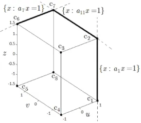
This complete the modeling procedure. Now, let us estimate the region of attraction of the nonlinear system (35)-(37) with respect to the origin by using its representation in the form of the NLDI model previously calculated. This was done using Lemma 5. In order to obtain a solution for the LMI (31), we have to describe the setXin the form given by (2). This was done by following the ideas presented in (Rohr et al., 2009). At first, notice that (50) is equivalent to a polytopeX ⊂R3 whose vertices are defined byΘ :={c1, c2, . . . , c8}, where
c1=
1 −π/2 −π/2
, c2=
1 −π/2 π/2
, c3=
−1 −π/2 π/2 ,
c4=
−1 −π/2 −π/2
, c5=
−1 π/2 −π/2
, c6=
−1 π/2 π/2 ,
c7=
1 π/2 π/2
, c8=
1 π/2 −π/2 .
A vertex representation ofX is defined as the convex hull ofc1, c2, . . . , c8,i.e.,X=Co(c1, c2, . . . , c8). Equivalently,
we can define this vertex form ofXas (2):
X :={x:akx≤1, k= 1, . . . ,12}. (54)
In order to calculate the vectorsak ∈ R3, notice that each
two vertices belongs to its edge, that is
c1, c2∈ {x:a1x= 1}, c2, c3∈ {x:a2x= 1},
c3, c4∈ {x:a3x= 1}, c1, c4∈ {x:a4x= 1},
c4, c5∈ {x:a5x= 1}, c5, c6∈ {x:a6x= 1},
c6, c7∈ {x:a7x= 1}, c7, c8∈ {x:a8x= 1},
c5, c8∈ {x:a9x= 1}, c1, c8∈ {x:a10x= 1},
c2, c7∈ {x:a11x= 1}, c3, c6∈ {x:a12x= 1}.
Figure 1 shows the setX with its vertices and illustration of some of its edges ({x : a1x = 1},{x : a7x = 1} and
{x:a11x= 1}).
Figure 1: RegionXwith its verticesc1, . . . , c8and illustration
of some of its edges ({x : a1x = 1},{x : a7x = 1} and
{x:a11x= 1}).
For a given setΘ, the row vectorsak can be determined by
solving the following set of linear systems:
a1c1= 1
a1c2= 1
a1(c1+2c2)= 1
,
a2c2= 1
a2c3= 1
a2(c2+2c3)= 1
,
a3c3= 1
a3c4= 1
a3(c3+2c4)= 1
,
a4c1= 1
a4c4= 1
a4(c1+2c4)= 1
,
a5c4= 1
a5c5= 1
a5(c4+2c5)= 1
,
a6c5= 1
a6c6= 1
a6(c5+2c6)= 1
,
a7c6= 1
a7c7= 1
a7(c6+2c7)= 1
,
a8c7= 1
a8c8= 1
a8(c7+2c8)= 1
,
a9c5= 1
a9c8= 1
a9(c5+2c8)= 1
,
a10c1= 1
a10c8= 1
a10(c1+2c8)= 1
,
a11c2= 1
a11c7= 1
a11(c2+2c7)= 1
,
a12c3= 1
a12c6= 1
a12(c3+2c6)= 1
,
yielding the following row vectors
a1=[ 0.29 −0.45 0 ], a2=[ 0 −0.32 0.32 ],
a3=[ −0.29 −0.45 0 ], a4=[ 0 −0.32 −0.32 ],
a5=[ −0.29 0 −0.45 ], a6=[ −0.29 0.45 0 ],
a7=[ 0 0.32 0.32 ], a8=[ 0.29 0.45 0 ],
a9=[ 0 0.32 −0.32 ], a10=[ 0.29 0 −0.45 ],
a11=[ 0.29 0 0.45 ], a12=[ −0.29 0 0.45 ].
The ellipsoidD :={x∈R3|x′P x≤1}was used for the
estimation of the region of attraction of the nonlinear sys-tem. To calculate the largest estimate in regionX, the LMIs of Lemma 5 were solved as an optimization problem by min-imizing the trace of matrixP. The calculated matrixPis
P =
0.307 −0.001 0.013
∗ 0.285 −0.031
∗ ∗ 0.301
.
Figure 2 shows the estimated region of attractionDand the state-space regionX defined as (50). It is important to em-phasize that D is an estimate of the region of attraction of the nonlinear system (35)-(37) with respect to the origin. It was calculated via Lemma 5 by using the representation of the nonlinear system in the form of the NLDI previously cal-culated.
Next section presents the theory towards the design tech-nique of the dynamic output feedback controller.
4
DYNAMIC OUTPUT FEEDBACK
CON-TROLLER DESIGN
Let the controlled system formed by the interconnection be-tween (5) and (6)-(7) (withy(t) =Cx(t)) be described as
˙˜
x(t) = ( ˜A0+ ∆ ˜A(t))˜x(t), (55)
where∆ ˜A(t) = ˜F E(t) ˜G, withE(t)satisfying∥E(t)∥≤1, for allt >0. Besides,x˜(t) = [x(t) xc(t)]′, and
˜
A0=
[
A0 BCc
BcC Ac ]
,F˜ =
[
F
0
]
,G˜=
[
G′
0
]′
.
In many applications, it is desirable that the system trajec-tories approach the origin as fast as possible (Folcher and Ghaoui, 1994; Silva and Junior, 2006). This practical re-quirement can be fulfilled by guaranteeing thatlimt→∞eαt∥
x(t)∥= 0 for all trajectories of (55), whereαis defined as being the decay rate of (55). This can be done by satisfying the conditionV˙(˜x(t)) ≤ −2αV(˜x(t))(Boyd et al., 1994), where V(˜x(t)) = ˜x(t)′P˜x˜(t) is the Lyapunov function
adopted to the NLDI model. This condition is equivalent to the existence of a positive definite symmetric matrixP˜ ∈ R(n+nc)×(n+nc)and matricesA
c,BcandCcsuch that
[ ˜
A′
0P˜+ ˜PA˜0+ ˜G′G˜+ 2αP˜ P˜F˜
∗ −I
]
≺0. (56)
In addition, it may be desirable that all modes of response (eigenvalues) of the closed-loop matrixA˜0have damping
ra-tios larger than a minimum, pre-defined value (see the ap-plications in (Ramos et al., 2004; de Oliveira et al., 2009)). To comply with this, we impose an additional restriction on the problem formulation using the regional pole placement (RPP) technique (Chiali et al., 1999). This technique consists in the definition of a region for pole placement in the com-plex plane where the design objective is fulfilled. This region is defined by all the complex numbers that have a damping ratioξhigher (or equal) thanξmin, and it can be viewed in
Figure 3, whereξminis the desired minimum damping ratio
for the eigenvalues of matrixA˜0andδ= cos−1ξmin. Note
that the damping ratio is a local property, which only makes sense when the trajectory is close enough to the equilibrium point of interest.
All the eigenvalues of matrixA˜0 are located within the
re-gion specified in Figure 3 if there exists a positive definite symmetric matrixP˜ and matricesAc,Bc andCc such that
(Chiali et al., 1999)
[
( ˜A′
0P˜+ ˜PA˜0) sin(δ) ( ˜PA˜0−A˜T0P˜) cos(δ)
∗ ( ˜A′
0P˜+ ˜PA˜0) sin(δ)
]
≺0.
(57)
Figure 3: Region for pole placement.
4.1
Robustness of the controller with
re-spect to the variations in the
operat-ing conditions of the system
To deal with the robustness of the controller with respect to the different operating points of the system, we obtain a description of the system (1) in a certain state-space re-gion around each equilibrium point of interest. The idea is to design a fixed parameter controller in the form (6)-(7) that exhibits an effective performance in all of these regions. This controller, however, must not change the equilibrium points of the open-loop sytem. In fact, once that a certain initial condition is within the region of attraction of a par-ticular equilibrium (say, xe1), then the control objective is
to force the system trajectories to approach the pointxe1as
fast as possible, in accordance to the practical requirements discussed in the previous section.
The set of resulting controlled systems are described in state space form by
˙˜
x(i)(t) = ( ˜A0i+ ∆ ˜Ai(t))˜x(i)(t), i= 1, ..., np, (58)
where ∆ ˜Ai(t) = F˜iEi(t) ˜Gi, with Ei(t) satisfying ∥
Ei(t)∥≤1, for allt >0. We also have
˜
A0i= [
A0i BiCc
BcCi Ac ]
,F˜i= [
Fi
0
]
,G˜i= [
G′ i
0
]′
,
˜
x(i)(t) =
[
x(t)−xei
xc(t) ]
,
beingxeitheithequilibrium point of interest of (1).
4.2
The complete control problem
definite symmetric matricesP˜i,i = 1, ..., np, and matrices
Ac,BcandCcof proper dimensions such that
[ ˜
A′
0iP˜i+ ˜PiA˜0i+ ˜GiTG˜i+ 2αP˜i P˜iF˜i
∗ −I
]
≺0, (59)
[
( ˜A′
0iP˜i+ ˜PiA˜0i) sin(δ) ( ˜PiA˜0i−A˜T0iP˜i) cos(δ)
∗ ( ˜A′
0iP˜i+ ˜PiA˜0i) sin(δ) ]
≺0.
(60)
Notice that (59)-(60) are bilinear matrix inequalities (BMIs), since there are cross-products among the controller variables (i.e., Ac, Bc andCc) and matrices P˜i, i = 1, ..., np. In
this paper, we apply a two-step separation procedure that allows to transform the BMIs (59)-(60) into a set of LMIs (de Oliveira et al., 2000). Basically, this separation proce-dure consists on the parameterization of some matrix vari-ables and the definition of some new varivari-ables.
5
SOLVING THE BMI PROBLEM: THE
TWO-STEP SEPARATION PROCEDURE
The concepts and procedures described in this section are derived from the ideas presented in (de Oliveira et al., 2000). Consider the set of BMIs (59)-(60). Let us assume that: (i)
˜
P = ˜Pi,i = 1, ..., np; (ii) the dimension of the controller
is equal to the dimension of the plant to be controlled,i.e., nc = n, and; (iii) the controller output matrixCc is
previ-ously known. Let us partionate the matricesP˜and its inverse
˜
P−1and define a matrixT˜as follows
˜
P =
[
X U
∗ X
c ]
,P˜−1=
[
Y Y
∗ Y
c ]
,T˜=
[
I I
∗ 0
]
,
whereX, U, Xc, Y, Yc∈ ℜn×nand the dimensions ofT˜and
its submatrices are implicitly determined byP˜. Moreover, the following changes of variables are carried out
V =U Bc, P =Y−1, S =AcTU′, (61)
where the dimensions of matricesV,P andS are implicity determined by the transformations.
Now, the set of BMIs (59)-(60) can be transformed into a set of LMIs. For that, multiplyP˜, (59) and (60) on the right and the left by T,diag[T, I] anddiag[T, T], respectively; introduce the new variables V,P andS, and simplify the expressions by algebraic manipulations, remembering that
˜
PP˜−1=I. The resulting set of LMIs are given by
[
P P
∗ X
]
≻0,
D11 D12 D13
∗ D
22 D23
∗ ∗ D
33
≺0, (62)
N11 N12 N13 N14
∗ N
22 N23 N24
∗ ∗ N
33 N34
∗ ∗ ∗ N
44
≺0, (63)
where,D11= ¯AT0iP+PA¯0i+GTi Gi+2αP,D12=P A0i+
¯
AT
0iX+CyiTVT +S+GiTGi+ 2αP,D13 =P Fi,D22=
AT
0iX+XA0i+V Ci+CiTVT+GTiGi+2αX,D23=XFi,
D33=−I,N11= ( ¯AT0iP+PA¯0i) sin(δ),N12= ( ¯AT0iX+
PA¯0i+CiTVT +Ssin(δ),N13 = ( ¯AT0iP−PA¯0i) cos(δ),
N14= ( ¯AT0iX−P A0i+CiTVT+S) cos(δ),N22= (AT0iX+
XA0i+CiTVT +V Ci) sin(δ),N24 = (AT0iX −XA0i+
CT
i VT−V Ci) cos(δ),N23=N14′ ,N33=N11,N34=N12,
N44=N22,A¯0i=A0i+BiCc,i= 1, ..., np.
Solving this set of LMIs in the matrices variablesV,P,S andX, the matricesAcandBcof the controller
(remember-ing that matrixCc must be pre-specified) can be calculated
by
Bc =U−1V, Ac=U−1S′, (64)
whereU =P−X. The success in solving this LMI problem depends, obviously, in a proper choice of matrixCc. In this
paper, we calculate this matrix by setting up a state feedback gainK, in which the control lawu(t) =Kx(t)stabilizes the system (5) and fulfills the constraints discussed in section 4. This matrixKcan be found by solving the following LMIs in the matrix variables L and Y (Ramos et al., 2004):
Y ≻0,
[
Q11 Q12
∗ Q
22
]
≺0,
[
R11 R12
∗ R
22
]
≺0, (65)
where, Q11 = Y AT0i +A0iY +LTBiT +BiL + 2αY,
Q12=Y GTi,Q22=−I,R11= (Y AT0i+A0iY+LTBiT+
BiL) sin(δ),R12= (Y AT0i−A0iY+LTBiT−BiL) cos(δ),
R22=R11,i= 1, ..., np.
Once we have solved this set of LMIs (65), it is setled Cc:=K, whereK=LY−1.
It is important to emphasize that given the non-convex na-ture of the undepinning BMI, we cannot guarantee that the LMI problem that is created by setting the matrix Cc ob-tained from the solution of the state feedback problem will always have a solution. Recent papers, however have shown that this heuristics for calculation of matrixCcprovides
sat-isfactory results for the overall design procedure, as seen, for example, in (Ramos et al., 2004; Ramos et al., 2005; Kuiava et al., 2009).
6
TESTS AND RESULTS
Consider the following nonlinear system:
˙
x1(t) = −1.35x2(t)−0.56x3(t) + 0.08x1(t) sin(x2(t))
0.22 sin3(x2(t)) + 1.35u(t) (66)
˙
x2(t) = 2.8x1(t)−0.45x2(t)−0.02x3(t)−
0.05 sin2(x2(t)) + 0.11 sin(x2(t)) sin(x3(t))−
0.05 sin3(x3(t)) + 0.7u(t) (67)
˙
x3(t) = x1(t) + sin2(x2(t)) cos(x3(t)) (68)
y(t) = x3(t) (69)
We consider three equilibrium points of interest: xe1 =
[0 0 0]T, x
e2 = [0.3074 2.1277 −4.2718]T andxe3 =
[−0.034 −0.5368 1.4405]T. The Jacobian matricesA
01,
A02andA03were calculated via Taylor series expansion of
system (66)-(68) around the equilibrium pointsxe1,xe2and
xe3, respectively. They are:
A01 =
0 −1.35 −0.56 2.8 −0.45 −0.02
1 0 0
,
A02 =
0.07 −2.01 −0.56 2.8 −0.46 −0.01 1 0.38 −0.65
(70)
A03 =
−4.09 −1.58 −0.56 2.8 −0.31 −0.05 1 −0.11 −0.26
.
An eigenvalue analysis shows that these three equilibrium points are all locally asymptotically stable. Our goal is then to design a dynamic output feedback controller that improves the decay rate of the system trajectories, as well as, the damp-ing ratio of these trajectories as they are approachdamp-ing the equilibrium points. For that, we first modelled the nonlin-ear system (66)-(68) via three NLDIs in the form (5), each one describing a certain neighborhood of the pointsxe1,xe2
andxe31.
Let us discuss the construction of an NLDI model describing a certain state-space region of the studied nonlinear system containing the equilibrium point at the origin. Then, the same approach was applied to determine the other NLDIs associ-ated to the pointsxe2andxe3. Applying the mean value
the-orem to the nonlinear system (66)-(68) with respect toxe1,
we have a reformulation of it in the form of the following LPV system
1
Section 3.5 provided a numerical example where all the steps of the modeling procedure were discussed in details. In the example of this section, our focus is on the control problem. Hence, we omit some details about the application of modeling procedure to the nonlinear system (66)-(68).
˙
x1(t)
˙
x2(t)
˙
x3(t)
=
=
θ11(t) −1.35+θ12(t) −0.56+θ13(t)
2.8 −0.45 +θ22(t) −0.02+θ23(t)
1 θ32(t) θ33(t)
x1(t)
x2(t)
x3(t)
+
1.35 0.7
0
u(t),
(71)
whereθij :ℜ+→[hij, hij],i, j= 1, ...,3.
The bounds hij and hij were specified by analysing the
mathematical expressions of the functionshij(t)(which are
calculated by (9)) considering the following state-space re-gion:
X1 := {[x1 x2 x3]′∈R3| −0.25≤x1≤0.25,
−0.25≤x2≤0.30,−0.3≤x3≤0.3}. (72)
The regionX1 was defined by considering it as being the
operating range with respect to the equilibrium point at the origin. Thus, we specified the following bounds for the non-zero functionshij(t): h11=−0.020, h11= 0.024, h12=
−0.236,h12=0.316,h13=−0.0025,h13=0.003,h22=−0.09,
h22 = 0.086, h23 =−0.05, h23 = 0.055, h32 = −0.48,
h32= 0.56,h33=−0.025andh33= 0.025.
The LPV system (71) has 7 non-zero functionshij(t), which
means that the corresponding set ΩP LDI has 128 vertices
(as defined by (16)). To complete the procedure, we have to calculate matricesF1andG1. Different from the numerical
example of section 3.5, all the equations of the system (66)-(68) are nonlinear. Hence, none of the elements ofF1 was
forced to be equal to zero. The dimension of this matrixF1
was settled to3×1. This dimension was chosen instead of
3×2or3×3in order to reduce the number of elements to be calculated by the LMI optimization problem. The dimension of matrixG1was chosen to be3×3.
By especifying these dimensions to matricesF1andG1,
ma-tricesW andV were defined as being a1×3full row rank matrix and a3×3symmetric matrix, respectively. From the solution of the optimization problem suggested in section 3.3 using the SeDuMi solver (Sturm, 1999) in conjunction with YALMIP (Lofberg, 2004) it was possible to obtain the fol-lowing matrices
F1=
72.78 20.65 29.03
, G1=
1.7·10−3 6.8·10−4 6.8·10−4
0 1.6·10−3 4.4·10−4
0 0 1.5·10−3
.
The NLDIs describing the system dynamics around the equi-librium pointsxe2andxe3were calculated considering,
re-spectively, the following regions:
X2 := {[x1 x2 x3]′∈R3|0.0075≤x1≤0.5074,
1.93≤x2≤2.53,−6.37≤x3≤ −4.12}, (74)
X3 := {[x1 x2 x3]′∈R3| −0.374≤x1≤0.176,
−0.7368≤x2≤ −0.1688,−0.71≤x3≤1.595}.
(75)
The resulting set of NLDIs are given in the form
˙
x(i)(t) = (A0i+FiEi(t)Gi)x(i)(t) +Bu(t), (76)
y(t) = Cx(i)(t), (77)
wherei= 1,2,3andx(i)(t) =x(t)−x
ei. In addition,A01,
A02andA03are given by (70), respectively;F1andG1by
(73) and the other matrices are
F2=
5.44 7.22 25.4
, G2=
4.9·10−3 4.4·10−4 3.8·10−3
0 5.2·10−3 3.2·10−4
0 0 5.1·10−3
,
(78)
F3=
2.58 24.2 36.2
, G3=
5.1·10−3 4.7·10−4 4.6·10−3
0 5.4·10−3 4.1·10−4
0 0 5.3·10−3
.
(79) Finally, matricesBandCare directly determined by looking the nonlinear equations (66)-(69).
Now, let us estimate the region of attractionD1of the
equi-librium pointxe1of the nonlinear system (66)-(69) using the
corresponding NLDI model previously calculated. This was done by using Lemma 5. As already shown in section 3.5 for the numerical example 1, we have first to describe the setX1
in the form of (2). This description can be obtained using the same procedure adopted for that example of section 3.5. As a result, we have a setX1described in the form given by (2),
where
a1=[ 2.00 −2.00 0 ], a2=[ 0 −1.64 1.97 ],
a3=[ −2.00 −2.00 0 ], a4=[ 0 −1.64 −1.97 ],
a5=[ −1.64 0 −1.97 ], a6=[ −1.64 1.97 0 ],
a7=[ 0 1.67 1.67 ], a8=[ 1.64 1.97 0 ],
a9=
[
0 1.67 −1.67 ]
, a10=
[
1.64 0 −1.97 ]
, a11=
[
1.64 0 1.97 ]
, a12=
[
−1.64 0 1.97 ]
.
Figure 4 shows the ellipsoidD1 and the state-space region
X1defined as (72).
Now, our goal is to design a dynamic output feedback con-troller to the nonlinear system (66)-(69) using a description of it in the form of (76)-(77). A decay rate of0.01 and a minimum damping ratio equal to 15% were imposed as de-sign objectives to the controlled system. The SeDuMi solver,
Figure 4: RegionX1(the box bounded by the faces in gray)
and the estimation of the region of attractionD1 (in red) for
the equilibrium point at the origin.
used in conjunction with YALMIP, was used to solve the set of LMIs related to this control problem. The calculated con-troller is given by
Ac=
−26.38 −12.85 −260.21
−105.5 −89.36 −90.68
−4.17 −3.18 −110.22
,
Bc=
260.5 98.76 110.5
, (80)
Cc = [
−9.55 −5.25 0.58 ]
. (81)
The performance of the controlled system was verified via nonlinear simulations. Figs. 5, 6 and 7 show the response of variablesx1(t),x2(t)andx3(t), respectively, with respect to
different initial conditions. It is interesting to observe that
Figure 5: Response of x1(t) for the initial condition x0 =
[0.2 0.3 0.1]T applied att= 0.
Figure 6: Response of x2(t) for the initial condition x0 =
[0.1 2.0 −4.0]Tapplied att= 0.
Figure 7: Response of x3(t) for the initial condition x0 =
[0.2 2.2 −4]Tapplied att= 0.
open-loop system. This result shows the effectiveness of the designed controller.
The region of attraction of the equilibrium pointx˜e1 of the
closed-loop nonlinear system, wherex˜e1 = [x′e1 0 0 0]′,
was also estimated using the corresponding NLDI model in the form of (58). For that, we defined the ellipsoidD˜1 :=
{˜x∈R6|x˜′P˜
1x˜≤1}.
Figure 8 shows the ellipsoidD˜1, considering the state of the
controller equal to zero. This plot corresponds to the cut of the actual estimate of ellipsoidD˜1in the hyperplane defined
by the system states. Hence, from the result shown in Figure 8, the effectiveness of the designed controller for the nonlin-ear system (66)-(69) is guaranteeded within the regionD˜1.
7
CONCLUSION
In the first part of this paper, a method to calculate the param-eters of an NLDI model was presented. The objective is to obtain a suitable linear representation of a nonlinear system for control purposes, in such a way that a linear controller can be designed to guarantee some desired features for the nonlinear closed-loop system. In the second part, a robust control design method, written in terms of LMIs was pre-sented, in order to design a linear dynamic output feedback
Figure 8: RegionX1 (the box bounded by the faces in gray)
and the estimation of the region of attraction D˜1 for the
closed-loop nonlinear system (in red) with respect to the equi-librium point at the origin.
controller for a nonlinear system using the NLDI model ob-tained by the approah proposed in the first part.
The numerical examples presented in the previous section have shown the effectiveness of the modeling and control approach proposed in this paper. However, it is important to emphasize that the application of the modeling procedure may be restricted to small and medium size systems, once that the number of vertices of the obtained PLDI may become excessively high as the number of system nonlinearities in-creases. With respect to the proposed control design, one of its difficulties is the requirement, due to the nature of the control problem formulation, that the order of the designed LDOF controller must be equal to the order of the system to be controlled. In order to achieve the goal of producing low order controllers (in the cases where the dimension of the system is sufficiently high), the control design may be combined with a final step of model order reduction.
possible extensions of this research foreseen to the sequence of this research.
ACKNOWLEDGE
The authors would like to thank the reviewers for their help-ful comments and suggestions.
The authors would like also to thank Prof. Luis Fernando Costa Alberto for providing the Matlab routines used for the estimates of the regions of attractions in examples 1 and 2.
REFERENCES
Basler, M. J. and Schaefer, R. C. (2008). Understand-ing power system stability, IEEE Trans. Indus. Appl. 44(2): 463–474.
Bernard, F., Dufour, F. and Bertrand, P. (1997). On the jlq problem with uncertainty,IEEE Trans. Automat. Contr. 42(6): 869–872.
Boyd, S., Ghaoui, L. E., Feron, E. and Balakrishnam, V. (1994). Linear Matrix Inequalities in System and Con-trol Theory, Society for industrial and applied mathe-matics.
Chen, B. S., Lee, C. H. and Chang, Y. C. (1996). H∞
tracking design of linear systems: adaptative fuzzy ap-proach,IEEE Trans. Fuzzy Syst.4(5): 32–43.
Chiali, M., Gahinet, P. and Apkarian, P. (1999). Robust pole placement in lmi regions,IEEE Trans. Automat. Contr. 44(12): 2257–2270.
Coutinho, D. F. and da Silva Jr., J. M. G. (2010). Computing estimates of the region of attraction for rational control systems with saturating actuators,IET Control Theory Applications4(3): 315–325.
de Oliveira, M. C., Geromel, J. C. and Bernussou, J. (2000). Design of dynamic output feedback decentral-ized controllers via a separation procedure,Int. J. Contr. 73(5): 371–381.
de Oliveira, R. V., Kuiava, R., Ramos, R. A. and Bretas, N. G. (2009). Automatic tuning method for the design of sup-plementary damping controllers for flexible alternating current transmission system devices,IET Gen., Trans. & Distrib.3(10): 919–929.
Folcher, J. P. and Ghaoui, E. L. (1994). State-feedback design via linear matrix inequalities: application to a benchmark problem,Proc. of the IEEE Conf. on Contr. Appl.
Hossain, J., Pota, H. R., Ugrinovskii, V. and Ramos, R. A. (2009). A novel STATCOM control to augment LVRT of fixed speed wind generators,Proc. of the IEEE Conf. on Dec. and Contr.
Hu, T. (2007). Nonlinear control design for linear differen-tial inclusions via convex hull of quadratics, Automat-ica43(4): 685–692.
Hu, X. B. and Chen, W. H. (2007). Model predictive control of nonlinear systems: stability region and feasible ini-tial control,Int. J. Automation and Comput.4(2): 195– 202.
Kiyama, T. and Iwasaki, T. (2000). On the use of multi-loop circle criterion for saturating control synthesis,System and Control Letters41: 105–114.
Kuiava, R., Ramos, R. A. and Bretas, N. G. (2009). Robust control methodology for the design of supplementary damping controllers for FACTS devices,Revista Con-trole & Automao20(2): 192–205.
Lofberg, J. (2004). Yalmip: a toolbox for modeling and opti-mization in matlab,Proc. of the CACSD Conf., Taipei, Taiwan.
*http://control.ee.ethz.ch/ joloef/yalmip.php
Montagner, V., Oliveira, R. C. L. F. and Peres, P. L. D. (2010). Relaxaes convexas de convergncia garantida para o projeto de controladores para sistemas nebu-losos de takagi-sugeno, Revista Controle & Automao 22(1): 82–95.
Mozelli, L. A., Palhares, R. M., de Avellar, G. S. C. and dos Santos, R. F. (2010). Condies lmis alternativas para sis-temas takagi-sugeno via funo de lyapunov fuzzy, Re-vista Controle & Automao21(1): 96–107.
Orsi, R., Helmke, U. and Moore, J. B. (2006). A newton-like method for solving rank constrained linear matrix inequalities,Automatica42(11): 1875–1882.
Polanski, A. (1997). Lyapunov function construction by linear programming, IEEE Trans. Automat. Contr. 42(7): 1013–1016.
Pyatnitskiy, E. S. and Rapoport, L. B. (1996). Criteria of asymptotic stability of differential inclusions and pe-riodic motions of time-varying nonlinear control sys-tems,IEEE Trans. Circ. Syst. I43(3): 219–229.
Ramos, R. A., Martins, A. C. P. and Bretas, N. G. (2005). Improved methodology for the design of power sys-tem damping controllers, IEEE Trans. Power Syst. 20(4): 1938–1945.
Rohr, E. R., Pereia, L. F. A. and Coutinho, D. F. (2009). Robustness analysis of nonlinear systems subject to state feedback linearization, SBA Controle e Automao 20(4): 482–489.
Silva, S. and Junior, V. L. (2006). Active flutter suppression in a 2-d airfoil using linear matrix inequalities tech-niques,J. Braz. Soc. Mech. Sci. Eng.28(1): 84–93.
Sturm, J. F. (1999). Using SeDuMi 1.02, a Matlab tool-box for optimization over symmetric cones, Optimiza-tion Methods and Software11(1): 625–653.
Tognetti, E. S. and Oliveira, V. A. (2010). Fuzzy pole place-ment based on piecewise lyapunov functions,Int. J. Ro-bust and Nonlin. Contr.20(1): 571–578.
Topcu, U. and Packard, A. (2009). Local stability analysis for uncertain nonlinear systems,IEEE Trans. Automat. Contr.54(5): 1042–1047.
Vidyasagar, M. (1993). Nonlinear systems analysis, Engle-wood Cliffs, N.J: Prentice Hall.
Xie, L. and de Souza, C. E. (1992). Robust control for linear systems with norm-bounded time-varying uncertainty,
IEEE Trans. Automat. Contr.37(8): 1188–1191.
Yfoulis, C. A. and Shorten, R. (2004). A numerical technique for the stability analysis of linear switched systems,Int. J. Contr.77(11): 1019–1039.


![Figure 6: Response of x 2 (t) for the initial condition x 0 = [0.1 2.0 − 4.0] T applied at t = 0.](https://thumb-eu.123doks.com/thumbv2/123dok_br/18973808.454646/15.892.522.771.216.459/figure-response-x-t-initial-condition-t-applied.webp)
