HYGOR PIAGET MONTEIRO MELO
NONLINEAR SCALING IN SOCIAL
PHYSICS
HYGOR PIAGET MONTEIRO MELO
NONLINEAR SCALING IN SOCIAL
PHYSICS
Tese de Doutorado apresentada ao Programa de P´os-Gradua¸c˜ao em F´ısica da Universidade Federal do Cear´a, como requisito parcial para a obten¸c˜ao do T´ıtulo de Doutor em F´ısica.
´
Area de Concentra¸c˜ao: F´ısica da Mat´eria Condensada.
Orientador: Prof. Dr. Jos´e Soares Andrade Junior
Nonlinear scaling in social Physics / Hygor Piaget Monteiro Melo. – 2016. 66 f. : il. color.
Tese (doutorado) – Universidade Federal do Ceará, Centro de Ciências, Programa de Pós-Graduação em Física , Fortaleza, 2016.
Orientação: Prof. Dr. José Soares de Andrade Júnior.
1. Sociofísica. 2. Leis de escala. 3. Eleições. 4. Alometria. I. Título.
HYGOR PIAGET MONTEIRO MELO
NONLINEAR SCALING IN SOCIAL
PHYSICS
Tese de Doutorado apresentada ao Programa de P´os-Gradua¸c˜ao em F´ısica da Universidade Federal do Cear´a, como requisito parcial para a obten¸c˜ao do T´ıtulo de Doutor em F´ısica.
´
Area de Concentra¸c˜ao: F´ısica da Mat´eria Condensada.
Aprovada em 26/08/2016
BANCA EXAMINADORA
Prof. Dr. Jos´e Soares Andrade Junior (Orientador) Universidade Federal do Cear´a (UFC)
Prof. Dr. Andr´e Auto Moreira Universidade Federal do Cear´a (UFC)
Prof. Dr. Saulo Davi Soares e Reis Universidade Federal do Cear´a (UFC)
Prof. Dr. Luciano Rodrigues da Silva
Universidade Federal do Rio Grande do Norte (UFRN)
e compreens˜ao durante todo meu doutorado.
Professores Dr. Andr´e Auto Moreira e Dr. Saulo Davi Soares e Reis pela oportunidade de colabora¸c˜ao e ajuda indispensav´eis na elabora¸c˜ao dessa tese.
Professores Dr. Hans Jurgen Herrmann e Dr. Hernan Makse pela oportunidade de colab-ora¸c˜ao.
Marianna Campos, por toda dedica¸c˜ao, companhia e paciˆencia durante todos esses anos. A todos os meus familiares, mas em especial aos meus pais Raimundo Rabelo Melo e Iracema Monteiro de Almeida Melo pela dedica¸c˜ao e apoio dados durante toda a minha vida.
A todos os meus amigos: Heitor Credidio, Diego Ximenes, Daniel Gomes, Daniel Marchesi, Davi Dantas, Diego Lucena, Diego Rabelo, Leandro Jader, Levi Leite, Rafael Alencar, Saulo Dantas, Vagner Bessa, Kau˜a Melo, Eduardo Araujo, Rilder Pires, C´esar Menezes. Todos os funcion´arios do departamento de F´ısica da UFC.
RESUMO
As aplica¸c˜oes da mecˆanica estat´ıstica no estudo do comportamento humano coletivo n˜ao s˜ao uma novidade. No entanto, nas ´ultimas d´ecadas vimos um aumento enorme do inter-esse no estudo da sociedade usando a f´ısica. Nesta tese, utilizando t´ecnicas da f´ısica, n´os estudamos leis de escala n˜ao-lineares em sistemas sociais. Na primeira parte da tese real-izamos a an´alise de dados e modelagem de elei¸c˜oes p´ublicas. Mostramos que o n´umero de votos de um candidato escala n˜ao-linearmente com o dinheiro gasto na campanha. Para nossa surpresa, a correla¸c˜ao revelou uma rela¸c˜ao de escala sublinear, o que significa que o ”pre¸co”m´edio de um voto cresce `a medida que o n´umero de votos aumenta. Usando um modelo de campo m´edio descobrimos que a n˜ao-linearidade emerge da concorrˆencia e a distribui¸c˜ao de votos ´e causalmente determinada pela distribui¸c˜ao do dinheiro gasto na campanha. Al´em disso, mostramos que o modelo ´e capaz de prever razoavelmente o n´umero final de votos v´alidos atrav´es de um argumento heur´ıstico simples. Por fim, apresentamos o nosso trabalho sobre alometria de indicadores sociais. N´os mostramos como homic´ıdios, mortes em acidentes de carro e suic´ıdios crescem com a popula¸c˜ao das cidades brasileiras. Diferentemente de homic´ıdios (superlinear) e eventos fatais em aci-dentes de carro (isom´etrico), encontramos um comportamento sublinear entre o n´umero de suic´ıdios e a popula¸c˜ao de cidades, o que revela uma poss´ıvel evidˆencia de influˆencia social na ocorrˆencia de suic´ıdios.
a novelty. However, in the past few decades we shaw a huge spike of interest on the study of society using physics. In this thesis we explore nonlinear scaling laws in social systems using physical techniques. First we perform data analysis and modeling applied to elections. We show that the number of votes of a candidate scales nonlinear with the money spent at the campaign. To our surprise, the correlation revealed a sublinear scaling, which means that the average “price” of one vote grows as you increase the number of votes. Using a mean-field model we find that the sublinearity emerges from the competition and the distribution of votes is causally determined by the distribution of money campaign. Moreover, we show that the model is able to reasonably predict the final number of valid votes through a simple heuristic argument. Lastly, we present our work on allometric scaling of social indicators. We show how homicides, deaths in car crashes, and suicides scales with the population of Brazilian cities. Differently from homicides (superlinear) and fatal events in car crashes (isometric), we find sublinear scaling behavior between the number of suicides and city population, which reveal a possible evidence for social influence on suicides occurrences.
LIST OF TABLES
1 We used the Akaike’s information criterion (AIC) to compare the two models: A (without competition) and B (with competition). The AIC lets us determine which model is more likely to describe correctly the data and quantify by calculating the probabilities and an evidence radio. The probability column shows the likelihood of each model to be the most correctly. The evidence radio is the fraction of Probability B by Probability A, which means how many times model B is likely to be
correct than model A. The AIC was applied in the log(data). . . p. 47 2 We used the Akaike’s information criterion (AIC) to compare the two
models: A (without competition) and B (with competition). The AIC lets us determine which model is more likely to describe correctly the data and quantify by calculating the probabilities and an evidence radio. The probability column shows the likelihood of each model to be the most correctly. The evidence radio is the fraction of Probability B by Probability A, which means how many times model B is likely to be
correct than model A. The AIC was applied in the log(data). . . p. 48 3 We used the Akaike’s information criterion (AIC) to compare the two
models: A (without competition) and B (with competition). The AIC lets us determine which model is more likely to describe correctly the data and quantify by calculating the probabilities and an evidence radio. The probability column shows the likelihood of each model to be the most correctly. The evidence radio is the fraction of Probability B by Probability A, which means how many times model B is likely to be
The probability column shows the likelihood of each model to be the most correctly. The evidence radio is the fraction of Probability B by Probability A, which means how many times model B is likely to be
LIST OF FIGURES
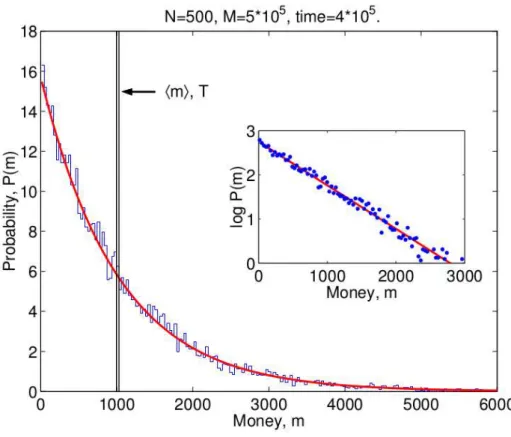
1 Histogram of money distribution. The blue line and points shows that the Boltzmann-Gibbs distribution emerges from a simulation of a economic model with money conservation. The vertical line shows the initial delta distribution of money. We see in the solid red line that an exponential function exp(−m/T) fits the data, where the money “tem-perature” is T = M/N, with the total money M = 5 . 105 and the
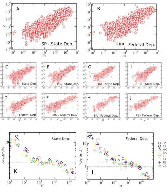
number of agents N = 500. This figure was taken from Ref. [19]. . . . p. 27 2 Scaling Relation between number of votes and money spent.
The red circles shows the relation between the number of votes and the declared campaign expenditure of each candidate in the state and fed-eral deputies elections in 2014 for the five largest states in Brazil: S˜ao Paulo (A,B), Rio de Janeiro (C,D), Minas Gerais (E,F), Bahia (G,H), and Rio Grande do Sul (I,J). Despite the large fluctuations, there is an unambiguous correlation between votes and money. In order to see the nuances of the correlation we plotted in (K) and (L) a normalized rela-tion for state and federal deputies for the eight largest states in Brazil. The symbols represents the normalized ratio hvi∆m/m where we first calculate the average number of votes in log-spaced bins along m. If we assume a linear correlation, the multiplicative constant is ∆m = M/n. The normalization provides us a direct observation of the nonlinearity in the dependence of votes on money. We see a global sublinear behav-ior, where the wealthier candidates display a lower fraction of votes per
log-spaced bins alongm. We see that our model shows a good agreement with the average behavior for all the money spectrum. In (C) and (D) we perform the same normalization process as in Fig.1, but now with ∆m estimated using Eq. 3.3. Each solid line shows the solution of our model, and the color indicates the state. Despite its simplicity, our model features all nonlinear regimes seen in the data, which corroborates our theory that the inefficiency of wealthier candidates are due mainly to
competition. . . p. 35 4 Frequency distribution of money and number of votes. In order
to derive the distribution of votes our model takes as input the distribu-tion of money. We see that the frequency distribudistribu-tion of money for the state deputies in S˜ao Paulo (A), Rio de Janeiro (B) and Minas Gerais (C) reveals a long tail characteristic that our model uses as an underly-ing cause for the observed vote distribution. We can now compare the actual distribution (black circles) of votes, P(v), with the obtained by our model (red diamonds) for the election of state representatives in S˜ao Paulo (D), Rio de Janeiro (E), and Minas Gerais (F). We can see that our model have a good agreement with the data showing that the uni-versal long tail characteristic of p(v) is a direct consequence of money
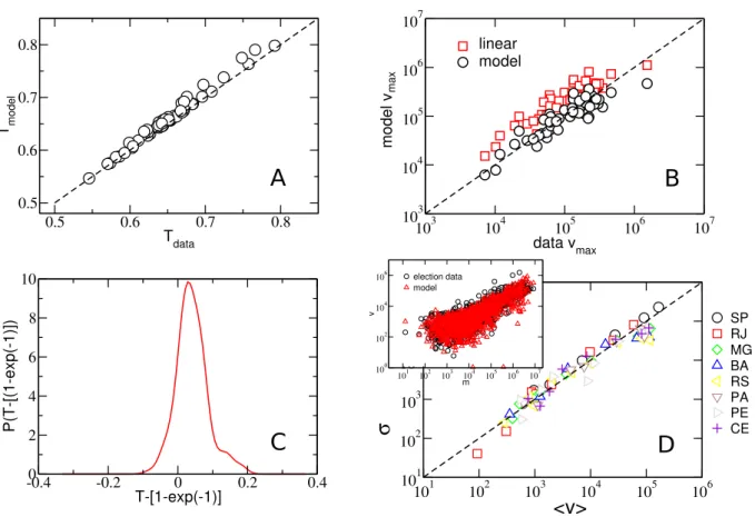
5 Analytical results of the model. By solving our model expressed in Eq. 1, we calculate the expected number of votes of each candidate. The total number of votes divided by the number of votersn is defined as the turnout ratioT. For all 56 parliamentary elections in 2014, we compared our model estimation of the turnout ratio, Tmodel, and the data ratio
Tdata, as we see in (A). The dashed line represents what would be the perfect agreement (Tdata=Tmodel) and we see that the simulations (black circles) exhibit a good agreement. We can also select the candidate with the largest number of votes vmax and see how our model estimate this
value. In (B) we see that our model (black circles) better estimates vmax
than the linear (red squares), which most of the time overestimates it. We show in (C) a histogram of T for the election of 2006, 2010, and 2014. We find an average turnout value of ≈ 67%, which is consistent with our heuristic estimation of T = 1−e−1
≈ 63%. We know that the exponential distribution have the property that the mean and standard deviation are equal, this property can be used in order to test if the dispersion along the mean follows an exponential distribution. In (D) we see that for state deputies of the eight largest states in 2014 election the data is in close agreement with the hypotheses of σ = hvi. We use the exponential distribution and the expected number of votes calculate by our model to generate a random election. We show in inset, for S˜ao Paulo, that when we add the random noise to our model (red triangle)
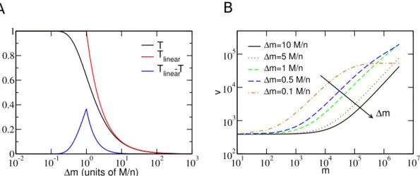
we obtain a cloud that closely resembles the actual data (black circles). p. 41 6 Dependence with ∆m. The solution of the mean field model
en-ables us to calculate the turnout radio T in function of the adimensional
n∆m/M parameter. In (A) we compare turnout for the approximated case where we excluded the competition between the candidates, Tgas, with the case with competition,T. The competition creates an exponen-tial saturation, which increases the loss of money when candidates seek new voters. This inefficiency is maximum when n∆m/M = 1.0, we can see that by looking for Tgas−T. We can also vary ∆m and see how the curve v(m) change. In (B) we show that as we decrease ∆m the values of v(m) usually increases, as expected by the definition of ∆m, however there is a point that we have a saturation process as the total number of
resents only one urban indicator, and the solid gray line indicate the best fit for a power-law relation, using OLS regression, between the av-erage total number of deaths and the city size (population). To reduce the fluctuations we also performed a Nadaraya-Watson kernel regres-sion [79, 80]. The dashed lines show the 95% confidence band for the Nadaraya-Watson kernel regression. The ordinary least-squares (OLS) [81] fit to the Nadaraya-Watson kernel regression applied to the data on homicides in (A) reveals an allometric exponent β = 1.24±0.01, with a 95% confidence interval estimated by bootstrap. This is compatible with previous results obtained for U.S. [6] that also indicate a super-linear scaling relation with population and an exponent β = 1.16. Using the same procedure, we findβ = 0.99±0.02 and 0.84±0.02 for the numbers of deaths in traffic accidents (B) and suicides (C), respectively. This non-linear behavior observed for homicides and suicides certainly reflects the complexity of human social relations and strongly suggests that the the topology of the social network plays an important role on the rate of these events. (D) The solid lines show the Nadaraya-Watson kernel regression rate of deaths (total number of deaths divided by the popula-tion of a city) for each urban indicator, namely, homicides (red), traffic accidents (blue), and suicides (green). The dashed lines represent the 95% confidence bands. While the rate of fatal traffic accidents remains approximately invariant, the rate of homicides systematically increases,
and the rate of suicides decreases with population. . . p. 55 8 Temporal evolution of allometric exponentβ for homicides (red
squares), deaths in traffic accidents (blue circles), and suicides (green diamonds). Time evolution of the power-law exponent β for each behavioral urban indicator in Brazil from 1992 to 2009. We can see that the non-linear behavior for homicides and suicides are robust for this 19 years period, and for the traffic accidents the exponent remain
9 Scaling relationship between suicides and population for US counties and MSAs. The small circles show the total number of sui-cides over five years (2003 to 2007) vs the average population for counties (A) and MSAs (B). The solid gray line indicate the best fit of a power law, using OLS regression, between the average total number of suicides and population. The dashed black lines delimit the 95% confidence band given by the Nadaraya-Watson kernel regression (solid black line) [79, 80]. The allometric exponents are obtained through an ordinary least-squares (OLS) fit [81] over the Nadaraya-Watson kernel regression applied to the suicides data. We find β = 0.87±0.01 for counties and β = 0.88±0.01 for MSAs with a 95% confidence interval estimated by bootstrap. The insets in each graph show the systematic decreases of suicide rates with
population in both cases. . . p. 57 10 Fatality per capita versus population for homicides, traffic
acci-dents, and suicides. The color map represents the conditional proba-bility density obtained by kernel density estimation. The bottom and top lines correspond to the 10% and 90% bounds of the distribution for each population size, that is 80% of the sampled points are between these lines. The middle line is the 50% level or ”median”expected for each population size. The diagonal shape observed in the left side of density maps are cases of low number of fatal events, one or two fatalities. After this region we observe that the three level lines wiggle around an average power-law behavior. In the case of homicides the three level lines indi-cate an increase in the expected density of fatality with the population size. Similarly, for traffic accidents the lines are close to horizontal, that is, the probability distribution for the rate of fatality is near indepen-dent of the population. For suicides, the median show a slight decrease with population size, while the 90% level, that is associated with cases of extreme rates of suicide, show a pronounced decrease. The sublinear growth observed for suicides, as depicted in Fig. 7C, is likely due to the
1 INTRODUCTION p. 16
2 BASIC CONCEPTS OF STATISTICAL MECHANICS p. 18
2.1 Statistical Physics . . . p. 20 2.1.1 Master Equation . . . p. 21 2.1.2 Equilibium . . . p. 22 2.2 Social physics . . . p. 24 2.2.1 Statistical Mechanics of Money Distribution . . . p. 25 2.2.2 Nonlinear Scaling . . . p. 26
3 THE ECONOMY OF ELECTIONS p. 30
3.1 Introduction . . . p. 30 3.2 Materials and Methods . . . p. 31 3.3 Empirical findings. . . p. 32 3.4 A mean field approach for the price of a vote . . . p. 35 3.5 Frequency distribution of votes . . . p. 38 3.6 Model validation . . . p. 38 3.7 Study of the dispersion . . . p. 40 3.8 Analytical Solution . . . p. 42 3.9 Comparing models . . . p. 45 3.10 Discussion . . . p. 51
4.1 Introduction . . . p. 52 4.2 Materials and Methods . . . p. 53 4.3 Allometry in Urban Indicators . . . p. 54 4.4 Discussion . . . p. 58
5 CONCLUSIONS p. 60
1
INTRODUCTION
Historically the origin of statistical mechanics is strongly connected with the study of statistical patterns of collective human activities. Maxwell and Boltzmann, the fathers of statistical mechanics, were greatly influenced by the emergence of new applications of probability theory on social data [1, 2]. However, it was only in the past few decades that the study of society using physics has been formalized and saw a huge spike of interest thanks to the large number of new social data produced by the Internet.
In this thesis we explore social systems using techniques commonly used in the physical sciences. The results is composed by two works [3] where we perform statistical data analysis and also a physical modeling approach. The main objective is to characterize and model the nonlinear scaling laws present at urban systems and elections.
This thesis is organized as follows: In Chapter 2, we present a short review on the introductory concepts of statistical mechanics and on its entangled history with statistics of social phenomena. As examples, we show how these concepts can be applied to two important problems: Distribution of money on a closed economical system, and the recent application of physics on the urbanization problem.
In Chapter 3, we study the scaling relation between the number of votes of a candidate and the amount of money spent at Brazilian legislative elections. Surprisingly, we find that the scaling is sublinear. This means that the price of a vote grows disproportionally with the number of votes, in such way that the richest candidates, on average, spend more for each vote than the less wealthy ones. To understand this observation we build a mean-field model that fits the relation between number of votes and money spent and allow us to explain this nonlinearity as a result of the competition among candidates.
17
massive relative to the size of the body as the body size increases [4]. However, the most prominent allometric relation was discovered by Max Kleiber in 1947 [5], between the metabolic rate of animals and their corresponding masses. More recently those ideas were extended to urban systems by Bettencourt et al. [6]. Here we show how homicides, deaths in car crashes, and suicides scales with the population of Brazilian cities. Our findings support the hypothesis that the number of suicides may be influenced by the non-trivial social substrate of cities.
2
BASIC CONCEPTS OF
STATISTICAL MECHANICS
Dealing with uncertainty is an unavoidable consequence of human nature. This hap-pens because science has the objective to explain, describe and predict natural phenomena and this always occurs under the state of reasoning with conditions of incomplete infor-mation. This lack of information happens in many levels and for many different reasons. Even if you take a simple length measurement with a rule, we know that different results will emerge in each try. This universal lack of information is represented in scientific theo-ries by randomness, and this universal aspect of nature is what gives the actual importance of statistics and probability theory.
Statistics originated in 17th century, motivated by the need to make sense of the social numbers collected by the increasingly bureaucratic state machine, such as the rates of death, birth, and marriage. The term statistics was introduced in the 18th century to denote these studies dealing with civil “states” [1, 2].
Inspired by the great success of Newton’s mechanics and astronomy, some scientists and philosophers start to seek immutable “natural” laws that governed human society. The French astronomer Pierre-Simon Laplace showed that the variations in male and female births and other social statistics could be described by a universal law, which we know today as Gaussian or normal distribution. This law was first proposed to describe the probabilities of coin tossing, which led Laplace to conclude that the birth of a male or female is a result of a random process, not a God’s desire to provide spouses for all. The success of Laplace’s studies on social data with the astounding ubiquity of the Gaussian curve of errors led the astronomer Adolphe Quetelet to write that
19
Statistical mechanics first appeared to deal with a specific type of uncertainty gen-erated by insufficient computational power. Before the discovery of quantum mechanics, physics was a deterministic science. However when you take a system with an enormous number of elements, there is a fundamental impossibility to solve all equations of motion. Even if it was possible, the amount of data generated would be intractable. Remarkably, this lack of information can be used as an advantage, the application of statistics on physi-cal system with huge number of elements shows that we can ignore most of the microscopic rules of interaction and, from an apparent microscopic randomness, emerges a homoge-neous system governed by simple mathematical laws. This new physical methodology is explained by James Clerk Maxwell when he came to study the problem of gases:
“...the smallest portion of matter which we can subject to experiment consists of millions of molecules, not one of which ever becomes individually sensible to us. We cannot, therefore, ascertain the actual motions of any one of these molecules; so that we are obliged to abandon the strict historical method, and to adopt the statistical method of dealing with large groups of molecules... In studying the relations between quantities of this kind, we meet with a new kind of regularity, the regularity of averages, which we can depend upon quite sufficiently for all practical purposes [8].”
The first contributions on the formal development of statistical mechanics were made by Daniel Bernoulli, James Clerk Maxwell, Ludwig Boltzmann, and Josiah Willard Gibbs in the second half of the nineteenth century. They were faced with the problem of explain-ing the empirical laws of thermodynamics by usexplain-ing the principles of Newtonian physics. To do so, they had to assume the existence of atoms and make extensive use of probability theory, a mathematical branch that can be traced back to mathematicians interested in maximizing their profit in games of change. These two ingredients produced a deep impact in science, initially with the creation of statistical physics and later with the application of this conceptual framework to interdisciplinary fields like biology, sociology, economy, etc [9, 10, 11, 12].
Even though one might think that Social Physics is a new endeavor, the two areas have intermingled and influenced each other since the times of Maxwell, as put by the science journalist Philip Ball [1]:
mo-of statistical physics, who found within it the confidence to abandon a strict Newtonian determinism and instead to trust to a ’law of large numbers’ in dealing with innumerable particles whose individual behaviors were wholly inscrutable.”
2.1
Statistical Physics
We mentioned that the creation of Statistical Mechanics was an effort to explain from first principles the origin of the experimental results of the Thermodynamics. This achievement came through by using two ingredients: the atomic hypotheses and the use of probability theory. Indeed, theses two ideas are close connected, because the macroscopic properties of the system can be computed by assigning a probability for each of the possible states accessible to the very large number of particles that compose it, without the need to solve their equations of motion.
A typical thermodynamical system is a gas. For instance, one liter of oxygen at standard temperature and pressure (T = 273,15K and p = 1.0Atm) consists of about 3×10²² oxygen molecules, all interacting with each other and colliding with the walls of
the recipient [13, 14]. Although the exact state of each atom is chaotic and unpredictable, the thermodynamic quantities, like volume or pressure, follow simple relations like Boyle’s law:
P V =constant. (2.1)
21
some strategies to determine such distributions over states, as we are going to describe next.
2.1.1
Master Equation
Suppose that we have a set of different systems, each one of many different random states. If we observe how they jump from one state to another, after some time we may see that the majority of systems would have converged to the same, most likely, state. This description is formalized by the method of solving a master equation.
Assume that our system is in a state i. The probability to find our system in a state
j after a time interval of dt is defined as Rijdt, where Rij is know as the transition rate fromi toj. Since we are interested in calculating which state is more likely, we have to define the probability of finding the system at state i at time t as pi(t). Therefore, we can use the transition rates to write down a master equation for the temporal evolution of pi(t):
dpi
dt = X
j
[pj(t)Rji−pi(t)Rij]. (2.2) The positive term represents the influx, the rate at which the systems are reaching statei
from every other statej, and the negative term is the outflux, the rate that the dynamics remove systems from state i. The set of probabilities also have to obey a normalization condition:
X
i
pi(t) = 1. (2.3)
The solution of Equation 2.2 with the normalization constraint gives us a method to find the distributionpi over time. The connection with the macroscopic reality is done by taking averages withpi. Suppose that you are interested in a macroscopic propertyM, if this property for each state i assumes the value of Mi, then the expected value of M at time t is
hMi=X i
we look Equation 2.2 we can see that, if for everyj the two terms on the right-hand side cancel one another, the probability distribution pi stops to evolve (dpi/dt = 0) and the system reaches a state called equilibrium state. Since equilibrium statistical mechanics is concerned only with the equilibrium state of systems, from now on we will write pi as a shorthand for limt→∞pi(t).
For a system in thermal equilibrium with a reservoir at temperatureT, Gibbs showed that the equilibrium distribution probability is
pi =
e−ǫi/kT
Z =
e−βǫi
Z . (2.5)
This is know as the Boltzmann-Gibbs distribution [14], where ǫi is the energy of state i and k = 1.38×10⁻²³
J/K is the Boltzmann’s constant. Using the convention β = 1/kT
we can write the normalization factor Z as
Z =X
i
e−βǫi
. (2.6)
The normalization factor Z is know as the partition function, and it has great signifi-cance on the mathematical treatment of statistical mechanics. The study of the variation of Z with parameters of the system, like temperature, gives us informations about the macroscopic properties.
From the Boltzmann-Gibbs distribution, Equation 2.5 together with Equation 2.4, we can calculate any macroscopic variable, for example, the expectation value of the energy
hEi, which in thermodynamics is defined as the internal energy U
U =hEi= 1
Z X
i
ǫie−βǫi, (2.7) and can also be expressed in function of the derivative of partition function with respect of β
U =−1
Z ∂Z
∂β =−
∂lnZ
∂β . (2.8)
23
internal energy, so we have
C = ∂U
∂T =−kβ
2∂U
∂β =kβ
2∂2lnZ
∂β2 . (2.9)
Basically the same procedure can be done to find any other thermodynamic parameter as a function of Z.
As we mentioned before, there are multiplies ways to derive the Boltzmann-Gibbs distribution. One of the most simple demonstrations is by dividing a system into two parts. Since the energy is additive, the total energy is the sum of the parts: ǫ =ǫ1+ǫ2,
whereas the probability is given by the product rule: p(ǫ) =p(ǫ1)p(ǫ2). The solution for
these equations is an exponential distribution, like in Equation 2.5.
Another derivation, proposed by Boltzmann, is a bit more complicated, but intro-duces new ideas that have a profound importance on the derivation of others equilibrium distributions. Take a system composed ofN particles, where each particle has an energy
ǫi. We call ni the number of particles in a single state ǫi, such that N = Pini and the total energy E =P
iniǫi. Consider that the system has a finite number of energy states with i ∈ [0, m]. The number of possible configurations Ω available for a fixed E that follows these two constraints is given by the combinatorial formula
Ω(E) = N!
n1!n2!n3!...nm!
. (2.10)
Assuming that every configuration {ni} has the same probability, to find the equilib-rium configuration we just need to find whichE maximizes Ω, which should be the most likely state. Boltzmann noted that instead of maximizing Ω, it would be much easier to maximize ln(Ω), because in the limit of large N we can use the Stirling approximation,
ni!≈e−ni nni
i , so
ln Ω
N =−
X i ni N ln ni N . (2.11)
ered by Shannon when working with information theory [15]. Since the probability is defined as pi = ni/N, we see that another equivalent definition for Entropy is S =
−P
ipilog(pi). The Shannon information entropy connected the information theory with statistical physics. This remarkable theory was responsible for the creation of a number of new interdisciplinary applications for statistical physics [10, 11, 16].
2.2
Social physics
The French political philosopher Auguste Comte in the 19th century first coined the term Social Physics [17, 1]. He believe that this new discipline should be the natural evolution in a search for a complete description of the world,
“Now that the human mind has grasped celestial and terrestrial physics, me-chanical and chemical, organic physics, both vegetable and animal, there re-mains one science, to fill up the series of sciences of observation – social physics. This is what men have now most need of; and this is the principal aim of the present work establish.”
As we mentioned before, the emergence of a Social Physics was a natural consequence of the creation of Statistical Physics. Unfortunately, this historical connection was lost for the most part of the 20th century. However, in the 90s, as the Statistical Physics was already well tested and matured, there was finally a movement towards applying its concepts to sociology and economy, mostly driven by the rapid evolution of computers and the huge amount of new social data available.
Applying statistical physics to model social dynamics involves two challenges. The first is finding a simple yet comprehensive microscopic model, and the second is finding how to extract the macroscopic behavior out of it. Solving the second problem is where lies the essence of what statistical physics has to offer to social science. A common mistake is to assume that the macroscopic behavior is a straightforward extrapolation of the individuals. The political scientist Michael Lind explains this problem [18]
25
in sufficient numbers, undergoes an astonishing change. They instinctively form a disciplined pack. Traditional political philosophers have been in the position of students of canine behavior who have observed only individual pet dogs.”
Despite of all complexity of the human interactions, the large-scale behavior seems to be independent of individual social characteristics, allowing us to use the same techniques to study of systems composed by a huge number of atoms or molecules [10]. In the following sections, we shall explore some examples of social phenomena that have been studied using the techniques of Statistical Physics.
2.2.1
Statistical Mechanics of Money Distribution
We saw that the fundamental law of equilibrium statistical mechanics is the Boltzmann-Gibbs law for the probability distribution of energy ǫ
P(ǫ) = e
−ǫ/kT
Z . (2.12)
The analytical derivation of an equilibrium distribution needs the imposition of con-straints, which usually is a conserved physical quantity, for instance, for the case of a Boltzmann-Gibbs distribution, we have to impose energy conservation.
Dragulescu and Yakovenko [19] took this classical mechanical assumption and applied it for a system of many economical agents that interact dynamically exchanging money, but the total amount of money is conserved. For simplicity, they assumed a closed system where the total amount of money is conserved, therefore, the equilibrium probability distribution of moneyP(m) is a Boltzmann-Gibbs distribution.
Let us suppose that we have a system with a constant number of agents and each agent i has some money mi from which a fraction can be exchange with other agents. First assume the simple case for the interaction ofiwithj, where the first pays an amount of money ∆m for some goods or services from j. The money balance should be written as
mi →m
′
i =mi−∆m,
mj →m
′
j =mj+ ∆m.
This local conservation is analogous to the transfer of energy from one molecule to another in molecular collisions of a gas.
Assuming money conservation and following the Boltzmann formalism, the distribu-tion of money m is given by the exponential [19]
P(m) = e
−m/T
Z , (2.15)
where the partition function Z = R∞
0 e
−m/T
dm = T, and T is an effective temperature, ormoney temperature, equal to the average amount of money per economic agent,
T =hmi=M/N. (2.16)
Here, M is the total money, andN is the number of agents.
It is possible to perform a simulation in order to verify if Equation 2.15 holds. If you give an initial amount of $1000 for all agents and at each time step you choose randomly two agents to perform an exchange of money ∆m, as shown in Equation 2.13, after a transient period, the money distribution should converge to the Boltzmann-Gibbs distribution. The simulated money distribution and theoretical curve are plotted in Figure 1. There is experimental evidence that the wealth and income distribution for the majority of the population indeed show this exponential distribution but followed by a power-law decay [11].
This simple example shows how to apply the concepts of statistical physics for a social system where the agents are exchanging not energy, but money. The application of physical concepts and techniques to Economics represents a vast and promising field, ranging from studying correlations in stock market series [20, 21], wealth distribution [22, 11], to the analysis of income distribution and inequality [23].
2.2.2
Nonlinear Scaling
27
Figura 1: Histogram of money distribution. The blue line and points shows that the Boltzmann-Gibbs distribution emerges from a simulation of a economic model with money conservation. The vertical line shows the initial delta distribution of money. We see in the solid red line that an exponential functionexp(−m/T) fits the data, where the money “temperature” is T = M/N, with the total money M = 5 . 105 and the number
of agents N = 500. This figure was taken from Ref. [19].
number of agentsN, usually persons for the case of social physics applications. Correctly assigning a size for a system is essential because comparing macroscopic variables of systems with different sizes can gives us important informations about how the agents interact.
In statistical physics we see that some measurable properties typically scale in propor-tion to the system size. An example is the energy, if we double the number of particles, the energy doubles as well. We call such physical properties as extensive. This means that if we have two systemsA andB, when we compose those two systems any extensive property should mathematically behave asf(A+B) =f(A) +f(B). Therefore, for those physical properties the whole is the sum of the parts.
c∝Lβ, (2.17) wherec is the specific heat, Lis the system size, and β is called a critical exponent.
In biology, the nonlinear scaling is called allometry. Allometry often implies the use of power-laws to describe the dependence of a wide range of anatomical, physiological and behavioral properties. Precisely, if we denoted Y a biological property and M the body mass of different animal species, one may find a relation in the form of Y ∝ Mβ. One of the most prominent allometric relations found in natural sciences is the so-called “three-quarters law” or Kleiber’s law [5], where the metabolic rate of animals should scale with exponentβ = 3/4 of their masses.
Inspired by biological laws, a group of physicists [6] showed that the cities belonging to the same urban system exhibit nonextensive rates of innovation, wealth creation, patterns of consumption, human social behavior, and several other properties related to the urban infrastructure. However, unlike in biology, they found that the scaling can be superlinear (β >1), linear (β = 1), and sublinear (β <1). Bettencourt and collaborators proposed a classification for the social variable in terms of the exponent [6, 24, 25]:
1. (β < 1) Sublinear scaling implies an economy of scale, because its per capita measurement decreases with population size. In the case of cities, for example, we see this type of scaling in the number of gasoline stations, the total length of electrical cables, and the road surface (material and infrastructure).
2. (β = 1) The linear (isometric) case typically reflects the scaling of individual human needs, like the number of jobs, houses, and water consumption.
29
3
THE ECONOMY OF
ELECTIONS
3.1
Introduction
Free and fair elections play a central role in democracy [28], exhibiting a complex process of negotiations between politicians and voters, with the past decades bearing witness to a steep increase in the expenditure of political campaigns. Take the example of the presidential elections in the US. The 1996 campaigns cost contestants approximately $123 million (corrected for inflation) all together, an amount that escalated to nearly $2 billion in 2012 [29]. Although campaign investments have grown, the impact of money into the electoral outcome remains not fully understood [30], and conclusions about the theme are quite contradictory. Some studies argue that incumbent spending is ineffective, and the challenger spending, on the other hand, produces large gains [31]. Others claim that neither incumbent nor challenger spending makes any appreciable difference [32], a theory that dates back to the 1940’s [33]. Yet another group argues that both challenger and incumbent spending are effective [34].
Despite the questioning about the effectiveness of political campaigns as a whole, the election campaign of President Barack Obama in 2012 spent more than 65% of its money on media, including TV and radio air time, digital and printing advertising, and others [35]. Therefore, the direct contact with voters not only figures as a major factor in campaign planning, but it is clearly believed to have relevant impact in succeeding to persuade undecided voters [36].
31
accurately reproduces the vote distribution P(v) when provided their money campaign distribution P(m). The model shows that the top vote-receivers are those who spend more in political campaign, but with a highly counterintuitive result: the more candidate spends, higher the price of a vote.
In Economics, a similar effect in which larger companies tend to produce goods at increased per-unit costs is known as diseconomy of scale, and it may have diverse causes like communication costs [37], and the Ringelmann effect, the psychological effect when individuals get less efficient when working in larger groups [38].
This diseconomy of scale is present on real data acquired from recent proportional elections in Brazil, openly available in [39]. As far as we know, this is the first work to report such phenomena in elections. The data is related to the elections for the national lower house and state congress in 2014. Brazilian representative elections are an excellent experiment due to a number of special factors. First, Brazil is a large country, both in population and land area. It has the fifth population of the world spread across roughly 8.5 million km2 (over 3 million mi2). Second, in contrast with executive elections,
representative elections in Brazil have a large number of candidates. Additionally, it is compulsory to vote in Brazil. Altogether, these factors leads to a huge data set from a quite diverse electorate.
We argue that competition between candidates is the root cause of this verified disec-onomy of scale in Brazilian elections, showing that a scenario without competition always overestimate the number of votes of top campaign spenders. Moreover, we show that the correct estimation of the approach with competition is able to reasonably predict the turnout rate of elections through a simple heuristic argument. Finally, we test our theory by using the principle of maximum entropy to show that the statistical dispersion of the model agrees with the one found in our data set.
3.2
Materials and Methods
State deputies are local representatives elected for a term of four years by a propor-tional system. His function is to legislate in the unicameral system of each state. The federal deputies are representatives in the chamber of deputies of the national Congress, one of the two houses of the legislative power. The number of elected federal deputies is proportional to the population of the state, from a total of 26 states and a federal district.
3.3
Empirical findings.
We start our analysis by assembling the data sets on the entire electoral outcome and campaign expenditure of candidates from all 26 Brazilian states. Figure 2 displays the number of votesvversus the declared campaign expendituremof each candidate in the top 5 Brazilian states by population: S˜ao Paulo (Figs. 2A and 2B), Rio de Janeiro (Figs. 2C and 2D), Minas Gerais (Figs. 2E and 2F), Bahia (Figs. 2G and 2H), and Rio Grande do Sul (Figs. 2I and 2J). Although spread, the clouds of points are neatly correlated and follow a clear trend. Remarkably, this trend is observed in all representative elections for all Brazilian states.
To extract the main relationship between v and m, we average the number of votes in log-spaced bins along m, which provides an estimation for the empirical relation of v
as a function of m. In order to plot in the same figure these results for different states, we perform a scale transformation on v by supposing simple linear relation v = c×m, wherecis a characteristic constant of a given election. If we define the average price of a vote as ∆m =P
imi/
P
ivi and suppose that it is roughly uniform across candidates, it is easy to see thatc= 1/∆m. If the relation between votes and money is linear then the plot of v×(∆m/m) should be a constant function ofm with value close to 1.0.
33
35
102 103 104 105 106
m 100 101 102 <v> ∆ m/m
101 102 103 104 105 106 107
m 100 101 102 103 104 105 106 v data <v> model
102 103 104 105 106 107
m 101 102 103 104 105 106 v data <v> model
102 103 104 105 106 107
m 100 101 102 <v> ∆ m/m SP RJ MG BA RS PA PE CE
A
B
C
D
State Dep. Federal Dep.
Federal Dep. State Dep.
Figura 3: Modeling the nonlinear scaling. In order to verify if our model correctly fits the data, we show in (A) and (B) the S˜ao Paulo election for state and federal deputies in 2014, respectively. Each small circle is one candidate and the red squares are the average number of votes in log-spaced bins alongm. We see that our model shows a good agreement with the average behavior for all the money spectrum. In (C) and (D) we perform the same normalization process as in Fig.1, but now with ∆m estimated using Eq. 3.3. Each solid line shows the solution of our model, and the color indicates the state. Despite its simplicity, our model features all nonlinear regimes seen in the data, which corroborates our theory that the inefficiency of wealthier candidates are due mainly to competition.
3.4
A mean field approach for the price of a vote
We consider an electoral process composed of two separate groups of individuals, candidates and voters. Alls candidates can compete for the vote of alln voters, and each candidatei has a limited moneymi to spend on their campaign. Thus, if at a given time
mi becomes null, the candidate will not be able to compete for voters anymore, so their number of votesvi stops varying.
dvi
dt = 1−
S(t)
n [mi(t)>0]. (3.1)
Where S(t) = Ps
i=0vi is the total number of decided voters at time t, and [mi(t)>0]
is the Iverson bracket, which is 1 if the condition inside the brackets is satisfied, and 0 otherwise. The right-hand side of the Eq. 3.1 is the probability of candidate i to choose an undecided voter at time t. Eq. 3.1 explicitly requires a definition for the rate of money expendituredmi/dt, in order to determine the end of the monetary resources of a candidate. Due to the nature of the problem, it is natural to expect thatdmi/dt <0. We choose the simplest case where the money decreases linearly at a constant ratio, in other words dmi/dt=−∆m. Additionally, we consider this ratio as uniform for all candidates. The probabilistic feature of Eq. 3.1 is central to confirm our hypothesis that electoral outcome is an output of campaign expenditure due to a competition process. To show that, we first consider the case without competition, where s≪n. Also, we assume here that n∆m ≫ mi for all i, so that the candidate with the largest money do not have enough money to reach out the whole network. By doing so, it is unlikely to a candidate to waste their campaign money on voter who’s already decided. Thus, the decided voters of other candidates do not affect the probability of candidate i to conquer an undecided voter, so vi replaces S(t) in Eq. 3.1, and the system of differential equations become uncoupled. Under this scenario, these equations are easily integrated, and the number of votes becomes vi = n−(n −v0,i)e−mi/n∆m. Here, v0,i is the initial number of votes of candidate i. Since n∆m ≫ mi, and assuming (n−v0,i) ≈ n, we find the linear form
of vi ≈ v0,i+mi/∆m by expanding the exponential function and taking its first order approximation. As we will discuss next, this simple model do not suffice to explain the whole complexity of the relation betweenv and m.
The first two regimes presented in Fig. 2 are understood by the analytical approach form above. For the regime of lowm, where the experimental data do not exhibit a clear correlation, the candidates start the race with v0,i votes. Since they cannot afford a long run and/or a large expenditure, their final performance fluctuates around the initial value
v0,i, which depends on different factors, such as free volunteer engagement. As campaign
money increases, the linear part overcomes the initial v0,i, and a linear regime emerges.
37
from the linear to the sublinear regime. This is done by solving Eq. 3.1 in its entirety. By integrating Eq. 3.1, we find
vi =v0,i+
mi ∆m −
1
n∆m Z mi
0
S(m′
)dm′
, (3.2)
where we identify that integrating the Iverson bracket over time we get the time length candidate i has to campaign, which is given by mi/∆m. Additionally, we changed the variable of integration on the last term by remembering thatdm′
/dt′
=−∆m. It is possible to find a differential equation for S(m′
) by taking Eq. 3.1 and summing over i. After solving it for S(m′
) and integrating the last term of Eqs. 3.2 (detailed solution can be seen at section 3.7), we find a set of nonlinear coupled equations that must be solved in a specific order, candidate by candidate, following an increasing order of mi. As a consequence, the number of votes of candidate i depends neither solely on
mi nor on t, but on the whole distribution P(m) through the integral at the right-hand of Eqs. 3.2.
Equation 3.2 has a simple interpretation. As in the scenario without competition all candidates begin their run with an initial number of votes, and those with sufficient money to keep running enter in a linear regime controlled by the second term of Eqs 3.2. Nonetheless, as we will see next, candidates with large enough money may start to waste their money on decided voters, fact expressed by the presence of S(m′
) on the last term of Eqs. 3.2, which encloses the competition dynamics. This collective influence of the campaign money from all candidates, Eqs. 3.2, is our second and most important result. It provides a bridge between campaign expenditure and electoral outcome and is the basis of the remaining results that follows.
In order to solve the model we have to use as inputs the money m of each candidate, an initial number of votes v0, the total number of voters n and ∆m. To definev0 we use
the average of votes for candidates with less thenR$1,000. For our model ∆m behaves as a free parameter that can be calculated in function of the turnout rateT =Sf/n, or final fraction of votes. This is possible because the total number of votes S(t) have a simple solution (see section 3.7) for the limitt→ ∞, and we can write the final fraction of votes as
T = 1−e−M/(n∆m)
. (3.3)
Where M = P
reveals a good agreement with the average of votes. For the region of small money we see that our model, like the data, predicts a constant behavior, v ≈ v0. After this region we
have an evident correlation between votes and money. In order to better see the nuances of the correlated region we plotted in Figure 3(C) and (D) the normalized ratiohvi∆m/m
for the eight largest Brazilian states. The symbols represents the data average and the lines show our model solution for each state identify by the color. For small and large values ofm, we clearly see that our model correctly predicts the deviation from the linear behavior,hvi∆m/m≈1.0.
3.5
Frequency distribution of votes
One of the first empirical investigations carried out by physicists concerning Brazilian elections was focused on the distribution p(v) of the number of candidates receiving v
votes. Since then, several other works have shown how the distribution changes for other countries [52, 59], and also proposed models to explain p(v) [45, 40]. For our model the distribution of votes is an outcome of the distributionp(m) of the number of candidates spendingm. In Figure 4(A), (B) and (C) we show the distributionp(m) for state deputies of S˜ao Paulo, Rio de Janeiro, and Minas Gerais, respectively. We see an apparent power law decay that expands over close of four orders of magnitudes. Using those distributions as input for our model we determinep(v) for each one of those elections. In Figure 4(E), (F) and (G) we compare the empirical votes distribution for each state with the one obtained by our model. We see how our model reproduces correctly the empirical distri-bution for over two orders of magnitude. But even more, the correct prediction of p(v) shows that the long tail, emblematic ofp(v), is not a consequence of networks or dynamic properties but mostly it comes from the money distribution.
3.6
Model validation
39
102 103 104 105 106
v 10-8 10-6 10-4 10-2 P (v) data model D
102 103 104 105 106 10-8 10-6 10-4 10-2 data model
102 103 104 105 106 10-8 10-6 10-4 10-2 data model E F
100 101 102 103 104 105 106 107
m 10-8 10-6 10-4 P (m ) São Paulo -1
100 101 102 103 104 105 106 107
m 10-8 10-6 10-4 P (m )
Rio de Janeiro
-1
102 103 104 105 106 107
m 10-8 10-6 10-4 Minas Gerais -1
A B C
São Paulo Rio de Janeiro Minas Gerais
P (m ) P (v) P (v) v v
Figura 4: Frequency distribution of money and number of votes. In order to derive the distribution of votes our model takes as input the distribution of money. We see that the frequency distribution of money for the state deputies in S˜ao Paulo (A), Rio de Janeiro (B) and Minas Gerais (C) reveals a long tail characteristic that our model uses as an underlying cause for the observed vote distribution. We can now compare the actual distribution (black circles) of votes,P(v), with the obtained by our model (red diamonds) for the election of state representatives in S˜ao Paulo (D), Rio de Janeiro (E), and Minas Gerais (F). We can see that our model have a good agreement with the data showing that the universal long tail characteristic ofp(v) is a direct consequence of money distribution and a competitive dynamic.
used Equation 3.3 to estimate ∆m. We also compared how good our model estimates the candidate with the highest vote,vmax. Figure 5(B) shows the calculatedvmax against the votes of the most voted candidate, where each black circles is an election. The red circles shows a linear approximation (vi ≈mi/∆m). We see that points of the mean-field model gather around the identity line showing a good agreement, demonstrating that our model is better than the linear model, which overestimate the votes (see section 3.8 for a statical comparison).
The Equation 3.3 shows that if we estimate ∆m before the election, we can forecast the turnout ratioT. Fortunately, we can build some simple economical assumptions that presents a good agreement with the data. If we imagine that the candidates know the total money,M, and the size of the electorate,n, we can assume that the most simple and equitable division of votes will occur if ∆m =M/n, in fact this is the first point where
agreement with the average turnout, which we find experimentally to be≈67%.
3.7
Study of the dispersion
. Our model allow us to calculate the mean or expected value of the number of votes. However, to fully describe the election we have also to study the statistical dispersion, which is given by the conditional probability distributionp(v|m). We can use the concept of maximum entropy probability distribution (MaxEnt) in information theory to guess which is thep(v|m) that maximize the Shannon’s Entropy [16]. Imposing only a constraint for the meanhvithe maximum entropy continuous distribution is exponential,
p(v|m) = 1
hvie
− v
hvi. (3.4)
41
-0.4 -0.2 0 0.2 0.4
T-[1-exp(-1)] 0 2 4 6 8 10 P(T-[(1-exp(-1)])
0.5 0.6 0.7 0.8
T data 0.5 0.6 0.7 0.8 T model
A
C
101 102 103 104 105 106
101 102 103 104 105 106
D
σ <v> SP RJ MG BA RS PA PE CE 101 102 103 104 105 106 107m 100 102 104 106 v election data model
103 104 105 106 107
data v max 103 104 105 106 107 m o de l vmax linear model
B
Figura 5: Analytical results of the model. By solving our model expressed in Eq. 1, we calculate the expected number of votes of each candidate. The total number of votes divided by the number of voters n is defined as the turnout ratio T. For all 56 parliamentary elections in 2014, we compared our model estimation of the turnout ratio,
Tmodel, and the data ratio Tdata, as we see in (A). The dashed line represents what would be the perfect agreement (Tdata =Tmodel) and we see that the simulations (black circles) exhibit a good agreement. We can also select the candidate with the largest number of votes vmax and see how our model estimate this value. In (B) we see that our model
(black circles) better estimatesvmax than the linear (red squares), which most of the time
overestimates it. We show in (C) a histogram of T for the election of 2006, 2010, and 2014. We find an average turnout value of ≈67%, which is consistent with our heuristic estimation of T = 1−e−1
competition, analogous to an interaction in a physical system. If we suppose that the number of candidatesNC is much smaller than the number of votersn, we can neglect the interaction between candidates and the system of differential equations became uncoupled:
dvi dt =
(n−vi(t))
n [mi(t)>0] (3.5)
These equations can be simply integrated, and the expectation for the number of votes in function of money is
vi(mi) =n−(n−vi(0))e−mi/(n∆m)
. (3.6)
We can assume that n∆m >> mi for any i, which means that the candidate with the largest campaign finance will not have enough money to reach out the whole system. Therefore, we can find a linear approximation for the dependence between votes and money:
vi(mi) = n−(n−vi(0))
1− mi
n∆m + m2
i
2∆m2n2 −...
, (3.7)
vi(mi)≈vi(0) + (n−vi(0)) mi
n∆m. (3.8)
Assuming n−vi(0)≈n, we finally find the linear approximation
vi(mi)≈vi(0) +mi/∆m. (3.9) Now we want to solve the competition equation system. Taking Equation 3.1 and summing overi we can find a differential equation for S(t) that can be easily integrated:
Nc
X
i=0
dvi dt =
dS
dt =
(n−S(t))
n
Nc
X
i=0
[mi(t)>0] (3.10)
dS
dt =
(n−S(t))
43
S(t) = n−(n−S(0)) exp
−1
n Z t
0
r(t′
)dt′
. (3.12)
Where r(t) =P
i[mi(t)>0] and can be interpreted as the number of candidates who still have money at time t, which depends solely on the distribution of money.
The Equation 3.12 enables us to determine the turnout rate T of the election in function of ∆m, the total money M = P
imi, and n. We just need to take the limit
t→ ∞ and by doing that we determine the value whereS saturates.
T = S(t → ∞)
n = 1−e
−M/(n∗∆m)
. (3.13)
To find Equation 3.13 we used the fact that R∞
0 r(t
′
)dt′
= M/∆m and we use the approximation n−S(0) ≈n. In order to understand this integral we have to remember the definition of r(t) and also the fact that dt =−dm/∆m. So the integral became
Z ∞
0
r(t′
)dt′
= Z ∞ 0 Nc X i=0
[mi(m′
)>0]dm′
/∆m, (3.14)
Z ∞
0
r(t′
)dt′
= Nc
X
i=0
mi/∆m=M/∆m. (3.15)
In Figure 6(A) we show the turnout rate T (Eq. 3.13) in function of ∆m, and com-pare with the case without competition (Tlinear), which is obtained by simple summing Equation 3.9 and taking S(0)≈0. The amount of votes (or money) lost by competition can be evaluated by looking at the subtraction of the two rates. We see that there is a maximum loss when ∆m = M/n. As we can observe, ∆m can work physically as an external field that will provide energy to the system in order to convince a fraction of the voters, or also ∆m can be seen as a Temperature, wherein for small values the system organize in a big cluster of convinced nodes and for large values of ∆m the system stay in a “disorganized” state (T ≈0).
Now we can integrate our model in function of S(t) and calculate v,
vi =vi(0) +
mi ∆m −
1 ∆m
Z mi
0
S(m′
)
n dm
′
Figura 6: Dependence with ∆m. The solution of the mean field model enables us to calculate the turnout radio T in function of the adimensionaln∆m/M parameter. In (A) we compare turnout for the approximated case where we excluded the competition between the candidates,Tgas, with the case with competition,T. The competition creates an exponential saturation, which increases the loss of money when candidates seek new voters. This inefficiency is maximum whenn∆m/M = 1.0, we can see that by looking for
Tgas−T. We can also vary ∆m and see how the curvev(m) change. In (B) we show that as we decrease ∆m the values ofv(m) usually increases, as expected by the definition of ∆m, however there is a point that we have a saturation process as the total number of votes starts to get close of the size of the system (T →1.).
vi(mi) = vi(0) + 1 ∆m
1− S(0)
n
Z mi
0
exp
"
− 1
n∆m Z m′
0
r(m′′
)dm′′ #
dm′
. (3.17)
To find an analytical expression for v we have to solve the integral Rm′
0 r(m
′′
)dm′′
inside the exponential. But first we can decompose the external integral as
vi =vi(0) + 1 ∆m
1− S(0)
n
Z mi−1
0
exp
"
− 1
n∆m Z m′
0
r(m′′
)dm′′ #
dm′
+ 1 ∆m
1− S(0)
n
Z mi
mi−1
exp
"
− 1
n∆m Z m′
0
r(m′′
)dm′′ #
dm′ ,
(3.18)
vi =vi(0)−vi−1(0) +vi−1+
1 ∆m
1− S(0)
n
Z mi
mi−1
exp
"
− 1
n∆m Z m′
0
r(m′′
)dm′′ #
dm′ .
45
definition of r(m) for the external interval m′
∈[mi−1, mi] we have that
Z m′
0
r(m′′
)dm′′
=m0+m1 +m2+...+mi−1+ (Nc−i)m ′
. (3.20) By solving the integrals we finally find that the number of votes vi is given by
vi =vi(0)−vi−1(0) +vi−1−
n−S(0)
Nc−i
e−Pi−1
j=0mj/(n∆m)[e−(Nc−i)mi
n∆m −e−
(Nc−i)mi−1
n∆m ]. (3.21)
We can see in Equation 3.21 that the number of votes of a candidate i is not only a function of his budget mi but indeed it depends of the set {mi}. We show in Fig. 6(B) how the curves v(m) changes in function of ∆m. As we decrease ∆m a large fraction of the system gets occupied, T → 1.0, and v(m) shows a curvature for larges values of m
and start to saturate displaying a nonlinear growth.
3.9
Comparing models
In order to compare the model with the simple case without competition we used the Akaike’s Information Criterion (AIC) [63]. AIC uses information theory to gives a relative estimation of the information lost when a given model is used to represent the process that generates the data. We used AIC to measure the relative quality of our model when we compare with the linear non-competitive model.
Lets suppose that we have a model, with k parameters, that fits a data set with N
points. If S is the residual sums of squares then the AIC is defined by
AIC =Nln
S N
+ 2(k+ 1). (3.22)
Using the Equation 3.22 we can calculate the AIC for each model and the preferred model is the one with the minimum AIC value. We define modelA as the model without competition andB the most complex model, where there is competition. The difference in AIC is defined as ∆AIC =AICB−AICA. With this difference we can calculate the probability that model B minimize the information loss:
PB =
e−0.5∆AIC
47
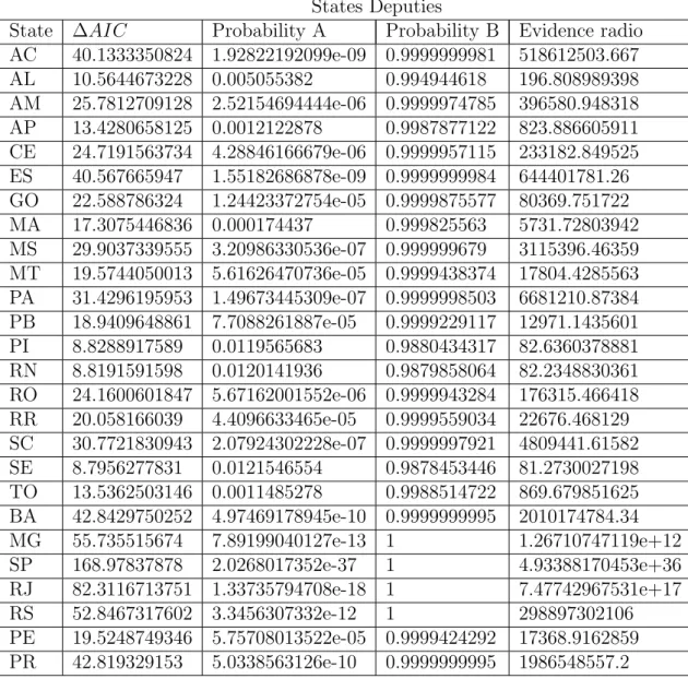
Tabela 1: We used the Akaike’s information criterion (AIC) to compare the two models: A (without competition) and B (with competition). The AIC lets us determine which model is more likely to describe correctly the data and quantify by calculating the probabilities and an evidence radio. The probability column shows the likelihood of each model to be the most correctly. The evidence radio is the fraction of Probability B by Probability A, which means how many times model B is likely to be correct than model A. The AIC was applied in the log(data).
Federal Deputies
Tabela 2: We used the Akaike’s information criterion (AIC) to compare the two models: A (without competition) and B (with competition). The AIC lets us determine which model is more likely to describe correctly the data and quantify by calculating the probabilities and an evidence radio. The probability column shows the likelihood of each model to be the most correctly. The evidence radio is the fraction of Probability B by Probability A, which means how many times model B is likely to be correct than model A. The AIC was applied in the log(data).
States Deputies
49
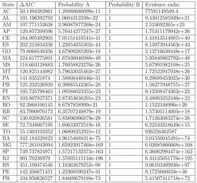
Tabela 3: We used the Akaike’s information criterion (AIC) to compare the two models: A (without competition) and B (with competition). The AIC lets us determine which model is more likely to describe correctly the data and quantify by calculating the probabilities and an evidence radio. The probability column shows the likelihood of each model to be the most correctly. The evidence radio is the fraction of Probability B by Probability A, which means how many times model B is likely to be correct than model A.
Federal Deputies
Tabela 4: We used the Akaike’s information criterion (AIC) to compare the two models: A (without competition) and B (with competition). The AIC lets us determine which model is more likely to describe correctly the data and quantify by calculating the probabilities and an evidence radio. The probability column shows the likelihood of each model to be the most correctly. The evidence radio is the fraction of Probability B by Probability A, which means how many times model B is likely to be correct than model A.
States Deputies
State ∆AIC Probability A Probability B Evidence radio AC 576.061906458 8.12356005108e-126 1 1.23098739187e+125 AL 238.628928458 1.52190160204e-52 1 6.57072703427e+51 AM 682.650418552 5.81226058412e-149 1 1.72050097467e+148 AP 358.738756255 1.26144655989e-78 1 7.92740677087e+77 CE 420.054263752 6.11470593755e-92 1 1.63540162064e+91 ES 480.640448515 4.26827816914e-105 1 2.34286510947e+104 GO 989.587809594 1.29938385781e-215 1 7.69595523285e+214 MA 519.730902297 1.38633608904e-113 1 7.21325808299e+112 MS 439.886900022 3.01837593293e-96 1 3.31303993347e+95 MT 310.209118004 4.35457632874e-68 1 2.29643465749e+67 PA 685.433108646 1.44574467234e-149 1 6.9168506662e+148 PB 400.461973128 1.09846804884e-87 1 9.10358750133e+86 PI 189.012621263 9.0454627114e-42 1 1.10552664016e+41 RN 249.978331952 5.2226980642e-55 1 1.91471915035e+54 RO 482.146906385 2.00969219136e-105 1 4.97588637852e+104 RR 370.038828903 4.4369982636e-81 1 2.25377595525e+80 SC 462.924309949 3.00098154818e-101 1 3.33224308096e+100 SE 139.093088068 6.2563306112e-31 1 1.59838100341e+30 TO 282.919902956 3.67048676832e-62 1 2.72443428656e+61 BA 642.920743716 2.46339667887e-140 1 4.0594355289e+139 MG 1450.44716375 1.09496501832e-315 1 inf
SP 2129.42600533 0 1 inf
RJ 1694.58149782 0 1 inf
51
3.10
Discussion
The nonlinear relation betweenv andmin real elections as a consequence of competi-tion between candidates can complement other statistical analyses for political campaign and electoral outcome [55, 54, 60]. These analyses detect a number of statistical patterns of electoral processes, such as the relations between party size and temporal correlations [61], the relations between the number of candidates and voters [58], and the distribution of votes [44, 56, 40, 52, 59]. Our analysis goes beyond these approaches by providing possible answers for a number of key issues: a simple equation that rationalize statistical evidence about the effects of political campaign on electoral outcome, an estimation for the ex-pected number of votes as a function of campaign money by accurately predicting the vote distribution, and finally a simple heuristic that can estimate the electorate turnout rate.
A close inspection of the campaign data reveals a ubiquitous nontrivial relation be-tweenv andmfor all elections investigated. We showed that this relation is an unambigu-ous sublinear correlation between the money spent by candidate and her/his number of votes v, specially for the the top spender candidates, revealing that the electoral process works in a diseconomy of scale state.
4
STATISTICAL SIGNS OF
SOCIAL INFLUENCE ON
SUICIDES
4.1
Introduction
It is not uncommon in nature to observe properties that present non-trivial forms of scale dependence. This is the case, for instance, of critical phenomena, where scaling invariance, universal properties and renormalization concepts constitute the theoretical framework of a well-established field in physics [69]. In biology, the so-called allometric relations certainly represent outstanding examples of natural scaling laws. Precisely, allometry implies the use of power-laws, Y ∝Mβ, to describe the dependence of a wide range of anatomical, physiological and behavioral properties, denoted here as Y, on the size or the body mass of different animal species, M. If the scaling exponent is β = 1, the variables Y and M are trivially proportional, and the relation between them is said to be isometric, while β 6= 1 indicates an allometric type of relationship. The so-called “three-quarters law” or Kleiber’s law, as originally proposed by the agricultural biologist Max Kleiber in 1947 [5], is surely one of the most prominent allometric relations found in natural sciences. Based on an extensive set of experimental data, this fundamental law states that the metabolic rate of all animals should scale to the 3/4 power of their corresponding masses [70, 4].