A Work Project, presented as part of the requirements for the Award of a Master Degree in Economics from the NOVA – School of Business and Economics
A Dynamic Panel Threshold model to analyse the Investment-Growth
nexus on a sample of Advanced Economies, Emerging Markets and
Developing Countries
António Pinto Ribeiro Student number 843
A Project carried out on the Master in Economics Program, under the supervision of: Prof. Paulo M. M. Rodrigues
A Dynamic Panel Threshold model to analyse the Investment-Growth
nexus on a sample of Advanced Economies, Emerging Markets and
Developing Countries
Abstract
This paper studies the Investment-Growth nexus, resorting to a Dynamic Panel Threshold model, for a sample of 12 Advanced, Emerging Markets and Developing Economies. The model estimated a 2.042% and 7.603% inflation threshold for Advanced Economies and for the Emerging Markets and Developing Economies, respectively. The impact of investment on GDP growth is significant and positive for Emerging Markets and Developing Economies in both inflation regimes, whereas for Advanced Economies positive significance is only observed when inflation is above the threshold.
1. Introduction
Policymakers aim to develop measures that allow for high and sustainable economic growth. Therefore, studying and understanding the impact of crucial variables on a country’s economic growth is vital and has been done for more than five decades. Hence, focusing first on the empirical literature related with the inflation-growth nexus it is possible to comprise and categorize the conclusions into four different predictions.
The first one states that inflation has no impact on growth (e.g., Dorrance, 1963; Cameron et al., 1996). For example, Sidrauski (1967) highlighted the super-neutrality of money, i.e., a monetary expansion would have no effect on growth since it would not change the steady state level of consumption.
The second one emphasizes the positive correlation between those two variables (e.g., Tobin, 1965; Shi, 1999). For example, Mallik and Chowdhury (2001) used cointegration and error correction models for four South Asian countries advising for the harm of very low inflation rates on the GDP growth rate.
and concluded that among other factors inflation harms per capita GDP growth by blocking savings and investment rates stimulation.
The fourth result emerged from a new strand of literature, highlighting nonlinearities in the inflation-growth relation. Fisher (1993) was one of the pioneers and concluded that there was a positive correlation when inflation was below a certain threshold and a negative one when above that (which weakened as inflation increased). Sarel (1996) examined this issue through the existence of a structural break on the function that relates inflation and growth. The author found a point of inflection at an average annual inflation rate of 8%, hence below that rate there is a slightly positive effect or no effect on growth whereas above the threshold it has a significant negative one.
One of the most important breakthroughs to study nonlinearities in the inflation-growth nexus was brought by Hansen (1999). The author introduced the panel threshold model and mitigated a crucial weakness that appeared in some of the previous analyses, by developing a method that allows for the estimation of a threshold instead of imposing one. Hansen’s contribution had some limitations since it imposed that all variables must be exogenous, ignoring the potential endogeneity bias of initial income (Caselli et al., 1996)1. Khan and Senhadji (2001) and Drukker et al. (2005) determined the inflation thresholds for a sample of 140 and 138 industrialized and developing countries, respectively. Khan and Senhadji (2001) estimated a threshold of 11%-12% for developing countries and 1%-3% for industrialized countries whereas Drukker et al. (2005) estimated two thresholds for industrialized countries of 2.57% and 12.61% and only one for developing countries of 19.16%. The two papers concluded that inflation above the thresholds (for both types of countries) will have a significant negative effect on growth. Bick (2010) extended Hansen’s (1999) work by accounting for regime intercepts for 40 developed
1 Drukker et al. (2005) and Omay and Kan (2010) coped with this problem by excluding initial income and Hineline
countries. He concluded that by allowing for regime intercepts the inflation threshold will be reduced from 19.16% to 12.03% and also showed that when inflation is above the threshold the negative impact of inflation on growth is only significant in the model that contains the regime intercept. Kremer et al. (2011) developed a Dynamic Panel Threshold model, allowing for endogeneity and fixed effects, estimating an inflation threshold for industrialized countries of 2.53% and one of 17.228% for non-industrialized countries. They concluded that inflation above the threshold has a negative impact on growth (for both types of countries), however below the threshold only for industrialized countries does it have a significant positive effect on GDP growth. Using the same approach, Vinayagathasan (2013) estimated a threshold of 5.43% for 32 Asian countries, concluding that above the threshold there is a significant negative effect on economic growth and below that there is no statistically significant effect.
Moreover, the panel data approach used by Drukker et al. (2005), Kremer et al. (2011) and Vinayagathasan (2013) also studied the impact of several other variables on GDP growth. Drukker et al. (2005) estimated, for a sample of non-industrialized countries, a significant negative impact of terms of trade and openness volatility on GDP growth, conversely to what happens with openness (in levels). He also found a positive relation between terms of trade volatility and GDP evolution in the industrialized sample. Kremer et al. (2011) estimated, for the sample of non-industrialized countries, a negative impact of population growth on GDP evolution and a positive nexus between openness volatility and growth for the sample of industrialized countries. Furthermore, the author estimated, for both industrialized and non-industrialized samples, a positive impact of investment and a negative impact of terms of trade on GDP growth. Vinayagathasan (2013) found the existence of a positive impact of investment and a negative impact of openness volatility on GDP growth for 32 Asian countries.
Threshold model for a sample of 6 Advanced and 6 Emerging Markets and Developing Economies from 1985 to 2014. The novelty presented in this paper, when compared with the model developed by Kremer et al. (2011) or Vinayagathasan (2013), is the substitution of the percentage of GDP dedicated to investment by inflation as a control variable. Therefore, the impact of investment on GDP growth will be estimated through two inflation regimes, whereas for the remaining variables (control variables) the impact will be estimated through a one-to-one relation with the GDP evolution. Furthermore, and in order to eliminate the country-specific fixed effects (Caselli et al, 1996) the Arellano and Bover (1995) methodology will be applied, i.e. the forward orthogonal deviations transformation. Moreover, to control for endogeneity a set of lags of the initial income as instruments will be used (Vinayagathasan, 2013).
The analysis performed throughout this paper, estimated an inflation threshold of 2.042% for Advanced Economies supporting Kremer et al.’s (2011) and Khan and Senhadji’s (2001) results. For the Emerging Markets and Developing Economies the threshold was 7.603%, which is lower than the one obtained by Kremer et al. (2011) and Khan and Senhadji (2001). For this type of countries, the relationship between investment and GDP growth is significant and positive in both inflation regimes, meaning that independently of the inflation level an increase in the amount of investment could always benefit GDP. Concerning the Advanced Economies, the positive impact on growth is only statistically significant when inflation is above the threshold.
The remainder of the paper is structured as follows. Section 2 presents and describes the data that was used in the model as well as the variables (and control variables) that were used. Section 3 presents a brief overview of the Dynamic Panel Threshold model that will be used, i.e., the econometrics behind the model construction and also the methods that allow us to solve some problems such as: fixed effects and endogeneity. Section 4 contains the estimation results for the Advanced Economies, and Emerging Markets and Developing Economies. Finally, section 5 provides concluding remarks and policy implications.
2. Data and Variables
The empirical analysis focuses on a balanced panel data approach that includes 12 countries for the period between 1985 and 2014. Concerning the data selection the procedure by Kremer et al. (2011) was followed and resorting to the International Monetary Fund (IMF) database it was possible to distinguish between Advanced and Emerging Markets and Developing Economies, of which 6 of each were chosen2.
The dataset for this work was extracted from the Peen World Table (PWT) 9.0, OECD, World Trade Organization and World Bank. Table 2, in the Appendix, presents the list of variables as well as the respective definitions and sources and Table 3 a country statistical summary. Notice that to smooth out business cycle fluctuations Vinayagathasan’s (2013) suggestion was followed and therefore all variables will be computed as two-year averages, thus instead of a time span of 30 observations for each country only 15 will be used.
The data shows that on average Advanced Economies have a lower inflation rate (4.10%) when compared to Emerging Markets and Developing Economies (75.58%). Moreover, the respective distributions are quite dispersed (see Figures 1 and 3 in the Appendix). Thus,
2 Advanced Economies: Germany; Spain; United Kingdom; Greece; Portugal and United States
according to Sarel (1996) the use of the log of inflation instead of the levels will provide a better fit for nonlinear models. Furthermore, it can, at least partially, mitigate the asymmetry characteristic of the initial inflation distribution, since specially for Emerging Markets and Developing Economies there will be some extreme observations (Ghosh and Phillips, 1998). Thus, following Khan and Senhadji (2001), to correct for negative inflation values, a semi-log transformation was used, i.e.,
𝜋̃𝑖𝑡 = {𝑙𝑜𝑔(𝜋(𝜋𝑖𝑡− 1), 𝑖𝑓 𝜋𝑖𝑡 ≤ 1% 𝑖𝑡), 𝑖𝑓 𝜋𝑖𝑡 > 1%
where 𝜋̃𝑖𝑡 represents an inflation function on which inflation rates below one follow a linear function, whereas above that level they are a logarithmic transformation. This method allows the inflation distribution to be less skewed and to be more in line with the normal distribution (see Figures 2 and 4 in the Appendix).
The study of the relationship between investment (inv) and economic growth (y) has to take into account that the second variable could influence and be influenced by other variables. Therefore, that matter shall be controlled. Hence, taking into consideration Kremer et al. (2011), Khan and Senhadji (2001) and Drukker et al. (2005) several control variables were used, namely, the initial income level (initial); the population growth rate (pop); the growth rate and standard deviation of the terms of trade (tot and sdtot); the level and standard deviation of openness (open and sdopen) and the difference when compared with the previously mentioned papers is the incorporation as a control variable of the inflation rate (𝝅)3.
3. The Dynamic Panel Threshold model
3.1The Econometric Approach
This empirical study will be based on a modification of the Dynamic Panel Threshold model developed by Kremer et al. (2011), which represents an extension of Hansen’s (1999) static
model. The difference between these models is the substitution of the percentage of GDP dedicated to investment by inflation as a control variable. Therefore, the impact of investment on GDP growth through two inflation regimes will be estimated, whereas for the remaining variables (control variables) the impact will be estimated through a one-to-one relation with the GDP growth evolution. Econometrically the Investment-Growth nexus can be represented as,
𝑦𝑖𝑡 = 𝜇𝑖+ 𝛽1𝑖𝑛𝑣𝑖𝑡𝐼(𝜋̃𝑖𝑡 ≤ 𝛾) + 𝛿1𝐼(𝜋̃𝑖𝑡 ≤ 𝛾) + 𝛽2𝑖𝑛𝑣𝑖𝑡𝐼(𝜋̃𝑖𝑡 > 𝛾) + 𝜙𝑋𝑖𝑡+ 𝜀𝑖𝑡. (1)
3.2Solving the Fixed Effects problem
The first step to estimate the model consists of the elimination of the country-specific fixed effects (𝜇𝑖). The longitudinal data literature offered several distinctive procedures to do it, from the usual first differencing (applicable in linear models) to individual means deviations (the within transformation). However, these kind of procedures, in a context of a Dynamic Panel Data Threshold model, would generate inconsistent estimators, since first differencing would produce negatively correlated error terms (and therefore Hansen’s (1999) distribution theory
would no longer be applicable), moreover the within transformation will always correlate the mean of individual errors with the dependent variable (Nickell, 1981). Therefore, a method is required that eliminates the country-specific fixed effects without interfering with Hansen’s (1999) distribution theory. Hence, following Arellano and Bover’s (1995) suggestion, the forward orthogonal deviations to mitigate the fixed effects problem were used. The forward orthogonal deviation transformation for the error term can be depicted as follows:
𝜀𝑖𝑡∗ = √𝑇−𝑡+1𝑇−𝑡 [𝜀𝑖𝑡−𝑇−𝑡1 (𝜀𝑖,(𝑡+1)+ ⋯ + 𝜀𝑖𝑇)].
Notice that this methodology does not affect the orthogonality of the transformed errors, 𝑉𝑎𝑟(𝜀𝑖𝑡∗) = 𝜎2𝐼
𝑇−1.
3.3Treating the Endogeneity problem
In the context of panel data, the use of endogenous variables in an OLS estimation framework leads to inconsistent estimators. Therefore, since in this empirical study the initial income level (initial) is a predetermined variable a set of instruments to surpass the endogeneity bias was used. More precisely, the lags of real per capita GDP (gdp) as instruments for the endogenous variable were used (Arrelano and Bover, 1995). Following Vinayagathasan (2013) and Kremer et al. (2011) all the available set of lags as instruments were applied, in a 𝑇 − 1 moment condition, i.e.,
𝑖𝑛𝑖𝑡𝑖𝑎𝑙𝑖𝑡 = 𝑔𝑑𝑝𝑖𝑡−1.
One important remark is the fact that the control variables were divided into two groups: 𝑋1𝑖𝑡 as the endogenous variable (initial) and 𝑋2𝑖𝑡 the remaining control variables.
For estimation a two stage least-squares (2SLS) approach was used. The first step can be characterized as the construction of the reduced-form for the endogenous variable (𝑋1𝑖𝑡∗ )which depends on the instrumental variables (𝑍𝑖𝑡) and exogenous variables considered (Caner and
Hansen, 2004), i.e.:
𝑋1𝑖𝑡∗ = 𝜆0+ 𝜆1∑𝑗=1𝑇 𝑍𝑖,𝑡−𝑗+𝜆2𝑖𝑛𝑣𝑖𝑡∗𝐼(𝜋̃𝑖𝑡≤ 𝛾) + 𝜆3 𝐼(𝜋̃𝑖𝑡≤ 𝛾) + 𝜆4𝑖𝑛𝑣𝑖𝑡∗𝐼(𝜋̃𝑖𝑡> 𝛾) + 𝜙′(𝑋2𝑖𝑡∗ ) + 𝜈𝑖𝑡. (3)
Least squares were used to compute the reduced-form parameters and the fitted values for 𝑋̂1𝑖𝑡∗ . The latter were used in the second step for the estimation of the model of interest (4), more precisely, the instrumental variable coefficients estimation.
𝑦𝑖𝑡∗ = 𝛽0+ 𝜌𝑋̂1𝑖𝑡∗ + 𝛽1𝑖𝑛𝑣𝑖𝑡∗𝐼(𝜋̃𝑖𝑡≤ 𝛾) + 𝛿1𝐼(𝜋̃𝑖𝑡≤ 𝛾) + 𝛽2𝑖𝑛𝑣𝑖𝑡∗𝐼(𝜋̃𝑖𝑡> 𝛾) + 𝜙′𝑋2𝑖𝑡∗ + 𝜀𝑖𝑡∗. (4)
Finally, the residual sum of squares (S) was computed depending on a specific 𝛾, as follows: 𝜀̂𝑖 = 𝑌 − 𝑋𝛽̂𝑖𝑣.
3.4Econometric Threshold Estimation
The inflation threshold level (𝛾) was estimated by conditional least squares. This methodology will minimize the residual sum of squares (RSS). As mentioned in the previous section the RSS depends on 𝛾, thus the inflation threshold level that will be chosen is the one that provides the smallest RSS value. Notice that this process will incorporate the whole range of inflation observations4. Moreover, the optimization process can be written as:
𝛾̂ = 𝑎𝑟𝑔𝑚𝑖𝑛 𝑆𝑛(𝛾)
𝛾 .
Furthermore, following Kremer et al. (2011) the inflation threshold’s 95% confidence interval were computed as:
Γ = {𝛾: 𝐿𝑅(𝛾) ≤ 𝐶(𝛼)}.
where 𝐶(𝛼)is the 95% percentile of the likelihood ratio’s (𝐿𝑅(𝛾)) asymptotic distribution. Once the instruments and 𝛾̂ are determined, GMM is used to estimate the slope of the coefficients from equation (1) and therefore the impact of those variables on GDP growth. From that, it will be possible to, for example, test whether or not both samples should have the same inflation threshold 5.
4 Hansen (2000) refers that it would be best to narrow the inflation range in order not to produce a too cumbersome
process. Even though this method was not used since it would reduce the sample and bias the analysis.
4. The Dynamic Panel Threshold model estimation results
4.1Advanced Economies
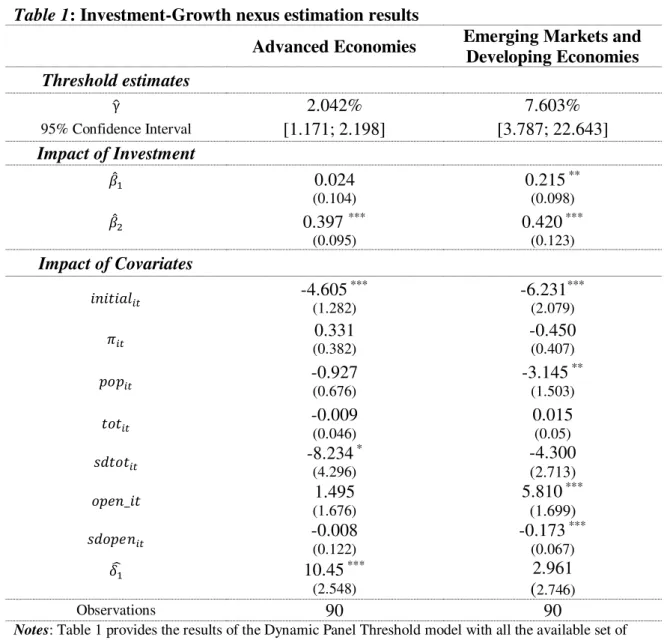
The results for the Investment-Growth nexus for the Advanced Economies are presented in the first column of Table 1. The estimated inflation threshold is 2.042% and the respective 95% confidence interval ([1.171; 2.198]) reinforces the inflation target of the European Central Bank as well as the Federal Reserve.
From the analysis of the two inflation regimes, low inflation regime (𝛽̂1) and high inflation regime (𝛽̂2), the results show that the relation between investment and growth is positive and statically significant only in the high inflation regime. This result is in line with the economic predictions, since it is expected that an increase (decrease) of one percentage point of the percentage of GDP dedicated to investment would impact positively (negatively) on GDP growth.
The initial income level (initial) detains a significant negative impact on GDP growth, following the conclusions reached by Vinayagathasan (2013). This result means that an increase of one percentage point in per capita GDP of the previous year generates a decrease in GDP growth of the current year.
theory. Note that the terms of trade (tot) can be thought of as the real exchange rate and thus sdtot as the volatility of real exchange rate. Therefore, it is expected that an increase of one
percentage point in the exchange rate generates a negative impact on GDP.
Table 1: Investment-Growth nexus estimation results
Advanced Economies Emerging Markets and
Developing Economies
Threshold estimates
γ̂ 2.042% 7.603%
95% Confidence Interval [1.171; 2.198] [3.787; 22.643] Impact of Investment
𝛽̂1 0.024
(0.104)
0.215 ** (0.098)
𝛽̂2 0.397 ***
(0.095)
0.420 *** (0.123)
Impact of Covariates
𝑖𝑛𝑖𝑡𝑖𝑎𝑙𝑖𝑡 -4.605
***
(1.282)
-6.231*** (2.079)
𝜋𝑖𝑡 (0.382) 0.331 -0.450 (0.407)
𝑝𝑜𝑝𝑖𝑡 -0.927 (0.676) -3.145
**
(1.503)
𝑡𝑜𝑡𝑖𝑡 -0.009 (0.046) 0.015 (0.05)
𝑠𝑑𝑡𝑜𝑡𝑖𝑡 -8.234
* (4.296) -4.300 (2.713) 𝑜𝑝𝑒𝑛_𝑖𝑡 1.495 (1.676)
5.810 *** (1.699)
𝑠𝑑𝑜𝑝𝑒𝑛𝑖𝑡 -0.008 (0.122) -0.173
***
(0.067)
𝛿̂1 10.45 ***
(2.548)
2.961 (2.746)
Observations 90 90
Notes: Table 1 provides the results of the Dynamic Panel Threshold model with all the available set of
4.2Emerging Markets and Developing Economies
The estimation results for the Emerging Markets and Developing Economies are displayed in the second column of Table 1. As expected the inflation threshold (7.063%) and the 95% confidence interval ([3.787; 22.643]) are higher than the ones estimated for the Advanced Economies.
The relation between investment and GDP growth is positive and statically significant in both low and high inflation regimes, which differs from the prior results for the Advanced Economies (in which the significance only emerges in the high inflation regime).
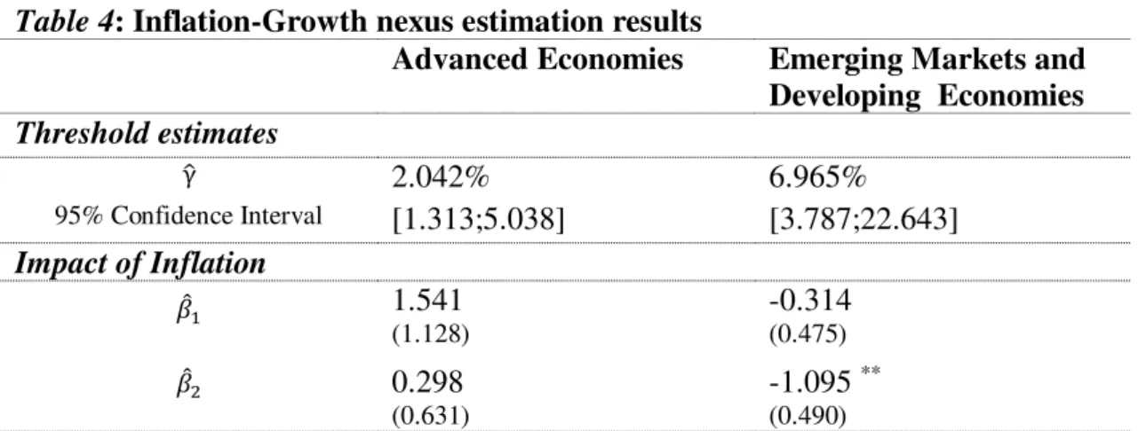
Similarly to the Advanced Economies results, inflation has not a statistically significant impact on GDP growth. Therefore, the relationship was analysed with Kremer et al.’s (2011)
methodology (as for the Advanced countries due to the same reasons). The results are presented in Table 4 and inflation has a significant negative impact on GDP growth in the high inflation regime. With this in mind, this set of countries should implement inflation targets not to harm the GDP growth.
Concerning the impact of the remaining covariates on GDP growth only the initial income level (initial); the population growth (pop) and openness’s level and volatility (open and sdopen) are significant. Moreover, the coefficients’ signs of those variables go towards the economic predictions.
5. Conclusion
The empirical analysis presented in this paper examined the Investment-Growth nexus for 6 Advanced and 6 Emerging Markets and Developing Economies, for the period from 1985 to 2014. The Dynamic Panel Threshold model, as described in section 3, was the econometric approach used to study the previous relation. The model described in this paper is based on the one used by Kremer et al. (2011) and Vinayagathasan (2013), but with the difference that it was built to study the relation between investment and GDP growth, and therefore, inflation is now a control variable and investment is estimated through a two inflation regime, as described in section 3. Following Kremer et al. (2011) the Arellano and Bover’s (1995) methodology was used, i.e., the forward orthogonal deviations transformation to eliminate the country-specific fixed effects and to deal with the endogeneity, that emerges from the initial income variable, was used based on a set of lags of the initial income as an instrument.
The estimation results found an inflation threshold of 2.042%, for Advanced Economies, which is in line with the Kremer et al.’s (2011) estimation and also the inflation target for the European Central Bank and Federal Reserve. Concerning the Emerging Markets and Developing Economies, the threshold estimated was 7.603%, which is lower than the one reached by Kremer et al. (2011). One possible explanation is related with the bigger sample (124 countries) that the author used as well as the period that is covered (1950 to 2004), on which the inflation, in this type of countries is characterized by being higher and volatile. Moreover, the fact that Emerging Markets and Developing Economies have a higher inflation threshold can be due to the use of an indexation systems.
Advanced Economies, the positive impact on GDP growth is only statistically significant when inflation is above the threshold.
Furthermore, the impact of inflation on growth was not statically significant in either of the two types of countries. However, Kremer et al.’s (2011) model was applied to corroborate if inflation could or not harm GDP growth and this led to the result that inflation harms GDP growth only for the case of Emerging Markets and Developing Economies when inflation is above the threshold.
Regarding the remaining control variables, only the terms of trade volatility and the initial income level were statically significant for the Advanced Economies whereas in the case of Emerging Markets and Developing Economies only the initial income level, the population growth and openness’s level and volatility impact upon GDP growth. Moreover, it shall be noticed that the signs of the previous significant coefficients were in accordance with economic predictions as well as with some of the conclusions of Kremer et al. (2011) and Drukker et al. (2005).
Notwithstanding, this paper detains its own limitations. First and foremost, the study only incorporates 8 explanatory variables, i.e., GDP growth could also be influenced by other variables. Second, in this empirical work only initial income was considered as endogenous, therefore the results can be biased if other control variables were considered as endogenous. Thus, in future works related with this matter the previous limitations should be taken into account as well as a larger sample.
Appendix
Table 2: List of Variables
Variable Description and Source
gdp
Two-year average of real GDP per capita (PPP) in 2011 constant price (in log). The annual real GDP per capita (PPP) 2011 constant price was computed as the expenditure-side real GDP at chained PPPs (in mil. 2011US$) divided by the population. Notice that was used the expenditure-side instead the output-side since the user guide of the Peen World Table 8.0 associates the first one to the one that generally is used to compute such measure. (Source: PWT 9.0)
initial
Two-year average of real GDP per capita (PPP) in 2011 constant price from the previous period (in log).
(Source: PWT 9.0)
y Two-year average of annual growth rate of real GDP per capita (PPP) in 2011 constant price. (Source: PWT 9.0)
pop Two-year average of annual growth rate of population.
(Source: PWT 9.0)
Two-year average of the annual percentage change of the consumer price index (CPI). (Source: OECD)
𝝅̃ Semi-log transformed .
inv Two-year average of annual GDP share dedicated to investment.
(Source: PWT 9.0)
tot
Two-year average of the annual percentage change in terms of trade (measured as exports divided by imports).
(Source: World Trade Organization)
sdtot Two-year standard deviation of the terms of trade.
open
Two-year average of log of openness (measured as the share of trade on GDP per capita (PPP) in 2011 constant price - trade is composed by exports plus imports).
(Source: World Bank)
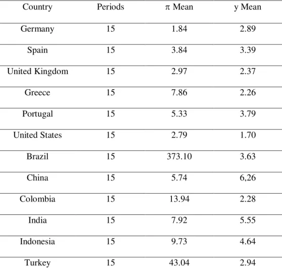
Table 3: Country Summary
Country Periods Mean y Mean
Germany 15 1.84 2.89
Spain 15 3.84 3.39
United Kingdom 15 2.97 2.37
Greece 15 7.86 2.26
Portugal 15 5.33 3.79
United States 15 2.79 1.70
Brazil 15 373.10 3.63
China 15 5.74 6,26
Colombia 15 13.94 2.28
India 15 7.92 5.55
Indonesia 15 9.73 4.64
Turkey 15 43.04 2.94
Notes: Table 3 contains the two-year average of annual growth rate of real GDP per capita
Table 4: Inflation-Growth nexus estimation results
Advanced Economies Emerging Markets and
Developing Economies
Threshold estimates
γ̂ 2.042% 6.965%
95% Confidence Interval [1.313;5.038] [3.787;22.643]
Impact of Inflation
𝛽̂1 1.541
(1.128)
-0.314
(0.475)
𝛽̂2 0.298
(0.631)
-1.095 **
(0.490)
Notes: Table 4 provides the results of the Dynamic Panel Threshold model with all the available set of
Figure 1: Distribution of Inflation Rate for Advanced Economies (in levels)
Notes: Figure 1 depicts the histogram of two-years average of annual Inflation rate (%) for Advanced Economies, 1985-2014. Source: OECD.
Mean 4.104670197
Median 2.8701215
Maximum 21.165065
Minimum -1.116687
Std. Dev. 4.09447743
Skewness 2.304804335
Kurtosis 5.395165685
Figure 2: Distribution of Inflation Rate for Advanced Economies (in semi-log)
Notes: Figure 2 depicts the histogram of two-years average of semi-log transformation of annual Inflation rate (%) for Advanced Economies, 1985-2014. Source: OECD.
Mean 1.040793927
Median 1.031844327
Maximum 3.048515621
Minimum -2.116687
Std. Dev. 0.877906864
Skewness -0.34575237
Kurtosis 1.507194654
Inflation Rate (%)
-2 0 2 4 6 8 10 12 14 16 18 20 22
F re q u e n c y 0 5 10 15 20 25 30 35 40
45 Figure 1: Distribution of Inflation Rate for Advance Economies (in levels)
Inflation Rate (%)
-2 -1 0 1 2 3
F re q u e n c y 0 5 10 15 20 25
Figure 3: Distribution of Inflation Rate for Emerging Markets and Developing Economies (in levels)
Notes: Figure 3 depicts the histogram of two-years average of annual Inflation rate (%) for Emerging Markets and Developing Economies 1985-2014. Source: OECD.
Mean 75.57518118
Median 8.550853
Maximum 2189.229
Minimum -0.5
Std. Dev. 318.6162255
Skewness 5.984667819
Kurtosis 36.41453593
Figure 4: Distribution of Inflation Rate for Emerging Markets and Developing Economies (in semi-log)
Notes: Figure 4 depicts the histogram of two-years average of semi-log transformation of annual Inflation rate (%) for Emerging Markets and Developing Economies 1985-2014. Source: OECD.
Mean 2.378744641
Median 2.109843899
Maximum 7.627364134
Minimum -1.5
Std. Dev. 1.488618544
Skewness 1.07762795
Kurtosis 3.314748892
Inflation Rate (%)
0 200 400 600 800 1000 1200 1400 1600 1800 2000 2200
F re q u e n c y 0 10 20 30 40 50 60 70 80 90
and Developing Economies (in levels)
Inflation Rate (%)
-2 -1 0 1 2 3 4 5 6 7 8
F re q u e n c y 0 5 10 15 20 25 30
References
1. Arellano, Manuel; Bover, Olympia. 1995. “Another look at the instrumental variables estimation of error component models”. Journal of Econometrics, 68: 29–51.
2. Barro, Robert. 1991. “Economic Growth in a Cross-Section of Countries”. Quarterly Journal of Economics, Vol. 106, No. 2, pp. 407–443.
3. Barro, Robert. 1996. “Inflation and economic growth”. Federal Reserve of St. Louis Review, 78: 153–169.
4. Bick, Alexander. 2010. “Threshold effects of inflation on economic growth in developing countries”. Economics Letters, 108: 126–129.
5. Bond, Stephen. 2002. “Dynamic panel data models: A guide to micro data methods and practice”. Working paper CWP09/02.
6. Cameron, Norman; Hum, Derek; Simpson, Wayne. 1996. “Stylized facts and stylized illusions: Inflation and productivity revisited”. Canadian Journal of Economics, 29: 152–162.
7. Caner, Mehmet; Hansen, Bruce. 2004. “Instrumental Variable Estimation of a Threshold Model”. Econometric Theory, 20: 813–843.
8. Caselli, Francesco; Esquivel, Gerardo; Lefort, Fernando. 1996. “Reopening the Convergence Debate: A New Look at Cross-Country Growth Empirics”. Journal of Economic Growth, 1(3): 363–389.
9. Christoffersen, Peter; Doyle, Peter. 1998, “From Inflation to Growth: Eight Years of Transition,” IMF Working Paper 98/99.
10.De Gregorio, José. 1992. “Effects of Inflation on Economic Growth: Lessons from Latin America”. European Economic Review, Vol. 36, pp. 417–25.
11.Dorrance, Graeme. 1963. “The effect of inflation on economic development”. IMF Staff Papers, 10: 1– 47.
12.Drukker, David; Gomis, Peres; Hernandez, Paula. 2005. “Threshold effects in the relationship between inflation and growth: a new panel-data approach”. MRPA Paper 38225, University of Munich, Germany.
13.Fischer, Stanley; Sahay, Ratna; Végh Carlos. 1996. “Stabilization and Growth in Transition Economies: The Early Experience”. Journal of Economic Perspectives, Vol. 10, pp. 45–66.
14.Fischer, Stanley. 1983. “Inflation and Growth”. NBER Working Paper No. 1235 15.Fischer, Stanley. 1993. “The role of macroeconomic factors in growth”. Journal of
Monetary Economics, 32(3): 485–511.
16.Ghosh, Atish; Phillips, Steven. 1998. “Warning: Inflation May Be Harmful to Your Growth”. IMF Staff Papers, Vol. 45, No. 4, pp. 672–710.
18.Hansen, Bruce. 1999. “Threshold Effects in Non-Dynamic Panels: Estimation, Testing, and Inference”. Journal of Econometrics, 93: 345–368.
19.Hansen, Bruce. 2000. “Sample splitting and threshold estimation”. Econometrica, 68: 575-603.
20.Hineline, David. 2007. “Examining the robustness of the inflation and growth relationship”. Southern Economic Journal, 73(4): 1020–1037.
21.Khan, Mohsin; Senhadji, Abdelhak. 2001. “Threshold effects in the relationship between inflation and growth”. IMF Staff Papers, 48(1):1–21.
22.Kremer, Stephanie; Bick, Alexander; Nautz, Dieter. 2011. “Inflation and Growth: New Evidence From a Dynamic Panel Threshold Analysis”, SFB 649 Discussion Paper 036
23.Levine, Ross; Zervos, Sara. 1993. “What we have learned about policy and growth from cross-country regressions”. American Economic Review, 83(2): 426–430.
24.Mallik, Girijasankar; Chowdhury, Anis. 2001. “Inflation and economic growth: Evidence from South Asian countries”. Asian Pacific Development Journal, 8: 123–135.
25.Nickell, Stephen. 1981. “Biases in dynamic models with fixed effects”. Econometrica, 49: 1417–1426.
26.Omay, Tolga; Kan, Elif. 2010. “Re-examining the threshold effects in the inflation-growth nexus with cross-sectionally dependent nonlinear panel:
Evidence from six industrialized economies”. Economic Modelling, 27: 996-1005. 27.Roodman, David. 2009. “A Note on the Theme of Too Many Instruments”.
Oxford Bulletin of Economics and Statistics, 71(1): 135–158.
28.Sarel, Michael. 1996. “Nonlinear Effects of Inflation on Economic Growth”. IMF Staff Papers, International Monetary Fund, Vol. 43, pp. 199–215.
29.Shi, Shouyong. 1999. “Search, inflation and capital accumulation”, Journal of Monetary Economics, 44: 81–103.
30.Sidrauski, Miguel. 1967. “Rational Choice and Patterns of Growth in a Monetary Economy". American Economic Review, 57(2): 534-544.
31.Stockman, Alan. 1981. “Anticipated Inflation and the Capital Stock in a Cash -in-Advance Economy". Journal of Monetary Economics, 8: 387-393.
32.Thanh, Su Dinh. 2015. “Threshold Effects of Inflation on Growth in the ASEAN-5 Countries: A Panel Smooth Transition Regression Approach”. Journal of Economics, Finance & Administrative Science, Vol. 20, pp. 41-48, 2015.
33.Tobin, James. 1965. “Money and economic growth”. Econometrica, 33: 671–684. 34.Vaona, Andrea; Stefano, Schiavo. 2007. “Nonparametric and Semiparametric