• Nenhum resultado encontrado

Estimating a Logistic Discrimination Functions When One of the Training Samples Is Subject to Misclassification: A Maximum Likelihood Approach.

N/A
N/A
Protected

Academic year: 2017

Share "Estimating a Logistic Discrimination Functions When One of the Training Samples Is Subject to Misclassification: A Maximum Likelihood Approach."

Copied!
9
0
0

Texto

(1)

Estimating a Logistic Discrimination

Functions When One of the Training Samples

Is Subject to Misclassification: A Maximum

Likelihood Approach

Nico Nagelkerke1*, Vaclav Fidler2

1Malawi-Liverpool-Wellcome Trust, Chichiri, Blantyre 3, Malawi,2Haren, Groningen, The Netherlands

*nnagelkerke@mlw.medcol.mw

Abstract

The problem of discrimination and classification is central to much of epidemiology. Here we consider the estimation of a logistic regression/discrimination function from training sam-ples, when one of the training samples is subject to misclassification or mislabeling,e.g.

dis-eased individuals are incorrectly classified/labeled as healthy controls. We show that this leads to zero-inflated binomial model with a defective logistic regression or discrimination function, whose parameters can be estimated using standard statistical methods such as maximum likelihood. These parameters can be used to estimate the probability of true group membership among those, possibly erroneously, classified as controls. Two exam-ples are analyzed and discussed. A simulation study explores properties of the maximum likelihood parameter estimates and the estimates of the number of mislabeled

observations.

Introduction

The problem of discrimination and classification has generated an extensive literature both from the biostatistical/epidemiological and from the machine learning communities. In its sim-plest form two populations, identified by a binary (dependent) variable y (y = 0 for controls or non-cases and y = 1 for cases,e.g. individuals with a specific disease), have to be distinguished on the basis of a set of p (e.g. genetic or behavioral) traits or (independent) (co)variablesx= (x1,..,xp)T,. In addition, the role of individual components ofxis often also of interest as this

may provide insight in the mechanisms that generate values of y; for example the role of a (mutant) gene in the etiology of a disease. A discrimination rule has to be estimated on the basis of a training sample of n = n0+n1observations, representative of the two underlying

pop-ulations; in machine learning terminology this is called supervised learning. Solutions range from classical Fisher Linear Discriminant Analysis and Logistic Regression to kernel based methods, Random Forests and Support Vector Machines. A nice overview is given by James

et al[1]. OPEN ACCESS

Citation:Nagelkerke N, Fidler V (2015) Estimating a Logistic Discrimination Functions When One of the Training Samples Is Subject to Misclassification: A Maximum Likelihood Approach. PLoS ONE 10(10): e0140718. doi:10.1371/journal.pone.0140718

Editor:Delmiro Fernandez-Reyes, University College London, UNITED KINGDOM

Received:June 22, 2015

Accepted:September 28, 2015

Published:October 16, 2015

Copyright:© 2015 Nagelkerke, Fidler. This is an open access article distributed under the terms of the

Creative Commons Attribution License, which permits unrestricted use, distribution, and reproduction in any medium, provided the original author and source are credited.

Data Availability Statement:All relevant data are within the paper, it Supporting Information files and fromhttp://faculty.washington.edu/norm/datasets. html.

Funding:The authors received no specific funding for this work.

(2)

A problem that, while surprisingly common in practice, has apparently attracted limited attention, is how to develop a discrimination rule when training samples have been“ contami-nated”by misclassification or mislabeling of the group membership. This type of misclassifica-tion is also known as“label error”or“label noise”. Mislabeling, that is misclassification of labels (i.e. the outcome or dependent y variable in the context of binary regression) may arise, for example, because the labeling involves some guesswork or subjective judgment as in medi-cal diagnoses. The presence of misclassification/mislabeling in training samples is often ignored in practice, or the problem is redefined in terms that fit available solutions. When researchers are aware of the problem it is also sometimes dealt with by removing or relabeling observations, either in anad-hocheuristic manner, or using an algorithm such as“depuration” that essentially removes“outliers”[2].

Some authors who explored this problem more formally were Lugosi[3], who explored this problem in the context of non-parametric pattern recognition, and Manevitz and Yousef [4], who explored this problem when only observations from one (sometimes misclassified) popu-lation are available. Some authors treated the“true label”as a latent or missing variable and used the EM algorithm for parameter estimation [5–6]. Some other authors considered the related problem of developing a discrimination rule when observations with a set of labels are available, only one of which is correct [7]. This situation of course is less relevant to the com-mon situation when only two labels are possible. In fact, in this situation,i.e. no information about the true label of any observation is available, the problem becomes a mixture analysis problem. Some authors considered the two possible labels mislabeling problem in the context of an underlying logistic regression function or discrimination rule. This is highly relevant for epidemiological case-control studies, where other types of discrimination rules cannot be esti-mated from this type of stratified samples. Nagelkerkeet alconsidered this in the context of “mixture”situations where no true labels are available [8]. As early as 1966 Lachenbruch explored the effect of mislabeling on Fisher's discriminant functions (also logistic functions), and found that, to first order, the effect is to shrink all coefficient towards the null with the same coefficient K and concluded that if some members of the original samples are incorrectly classified the utility of the discriminant function may not be seriously affected [9]. This how-ever, is not relevant if interest is in the values of the coefficients, or if the probability of the true label is important, as is the case in medical decision problems. For example, correctly estimat-ing the probability of seminal vesicle involvement in prostate cancer is key in makestimat-ing optimal therapeutic decisions. More recently, Albertet al[10] considered this mislabeling problem in situations in which there is a subsample with known true case status. Bootkrajang and Karan thoroughly addressed the mislabeling problem in the context of logistic discriminant rules in its most general form and explored, as we shall do for the one-sided (misclassifications occur in one direction only) problem, likelihood estimators for the parameters of the underlying logistic function [11–13].

Here we want to discuss the situation when only one of the training samples, in particular the control sample (but this is arbitrary of course), contains a non-negligible proportion of the other group (here cases). We assume that the underlying true discrimination rule–in which we are interested–is a logistic one.

(3)

strains. However, such control strains clearly do not exist, and instead environmental samples, comprising of a mixture of non-pathogenic and pathogenic strains, are used as controls.

This one-sided mislabeling problem however is very common. In data from health surveys, one can only compare people reporting hypertension, almost all of whom probably having this condition, to those who do not. A substantial proportion, however, of hypertensives may not be aware of their condition and are thus mislabeled as normotensives. In criminology, one can easily compare individuals convicted of a specific crime (say burglary) to those who have not, although many burglaries never result in convictions. Another common situation where this occurs is in the context of determining the sensitivity and specificity of a (new) test, when the putative gold standard itself has imperfect specificity or sensitivity. This is the case, for exam-ple, in tuberculosis, where culture is traditionally considered the gold standard, although there may be false-negative culture results [14]. Ignoring this problem may often be undesirable as in our legionella example where identifying strains as pathogenic may lead to costly public health interventions. It also has implications for the performance of classification methods. For exam-ple, boosting methods that iteratively increase the weight of misclassified observations may not work properly, and thus should either be avoided or applied asymmetrically, as argued by Long and Servedio [15].

Methods

Consider a population of stratified training samples, z = 0 and z = 1, sampled in the propor-tions n0:n1from the populations of possibly contaminated controls and cases. Denoting by

y = 1 the true cases and by y = 0 the true controls, we have P(y = 1|z = 1) = 1 and P(y = 1| z = 0)0, that is all observations with z = 1 are actually y = 1, but a possibly positive fraction of those with z = 0 is actually y = 1. Consequently, there will also be a positive probabilityλ= P (z = 0|y = 1,x) (assumed to be independent ofx). This probability depends both on P(y = 1| z = 0), which is assumed to be a fixed parameter, and the population mixing proportion n0:n1.

Here we consider this problem in the context of logistic regression. That is we assume that

Pðy¼1jxÞ ¼expðb0þβTxÞ=ð1þb0þβTxÞ

whereβ= (β1,. . .,βp)Tandβ0obviously depends on the proportion of true cases (y = 1) in the

total sample. For the probabilities of z conditional onxwe have

Pðz¼1jxÞ ¼Pðz¼1jy¼0;xÞ Pðy¼0jxÞ þPðz¼1jy¼1;xÞ Pðy¼1jxÞ

which in the case of an underlying logistic regression function becomes

ð1 lÞ expðb0þβTxÞ=ð1þb

0þβ

TxÞ

Similarly,

Pðz¼0jxÞ ¼Pðz¼0jy¼0;xÞ Pðy¼0jxÞ þPðz¼0jy¼1;xÞ Pðy¼1jxÞP

which again, by assuming a logistic regression function, becomes

½1þlexpðb0þβTxފ=ð1þb

0þβ

TxÞ

(4)

examples, the number of covariables p is large compared to n0+n1estimation (regularization)

methods penalizing model complexity,e.g. the lasso which penalizes the absolute values of the

βcoefficients (theλshould perhaps not be penalized), should be used (we did not as we consid-ered only few covariables).

As P(y = 1) = P(z = 1,y = 1)+P(z = 0,y = 1) = P(z = 1) +λP(y = 1), we have P(y = 1) = P (z = 1)/(1-λ). Thus the expected number of cases in the total sample equals n1/(1-λ), and the

expected number of controls who are actually cases is n1λ/(1-λ).

The parametersβ0,βin the defective logistic regression model are identical to the ones in

the underlying logistic model for y. Thus the latter model can be used for classification. (Asβ0

depends on the arbitrary mixing proportions of cases and controls these probabilities should be interpreted cautiously.). As our objective is the prediction (classification) of the y (instead of the observed, but possibly mislabeled, outcomes z) values of the observations, techniques such as cross-validation to explore the performance of our proposed method in given empirical con-texts, are not meaningful. Cross-validation would require a subset of observations, not used in estimating the classification function, for which the true, or gold standard, outcomes are known. This is obviously not the case.

Results

We apply our proposed method to two examples. In both examples we used the mle() function from the stats4 library of the statistical package R [17] for ML estimation of the DLR parame-ters. The loglikelihood, as usual, is the sum over all observations of {zlog(P(z = 1|x)) + (1-z)log (P(z = 0|x)}. Use of the maximum likelihood guarantees that–if the model is correctly speci-fied–the parameter estimators have well established nice properties such as consistency and (asymptotic) efficiency [18]. Also, criteria such as AIC, BIC, significance testing, etc. for decid-ing which elements ofxto include in the (final) model, can be used. However, we advise to base the decision to use defective logistic regression instead of standard logistic regression on prior, substantive, knowledge that non-negligible mislabeling occurs. This is, because standard asymptotic theory makes the assumption that the true parameter valueλlies away from the boundaryλ= 0.

We used the solutions of the standard logistic regression, that is the maximum likelihood solution when fixingλ= 0, as starting values. These starting values will guarantee convergence to a (possibly local) maximum with a likelihood at least as large as that of the standard logistic model. It is also possible to plot the profile likelihood ofλ(i.e. the maximum likelihood–over

β-for given values ofλ) to ensure that the likelihood is well-behaved in the relevant region of the parameter space. Where appropriate, as in example 2, we also boundedλby 0 below and by n0/(n0+n1) above using the L-BFGS-B method.

As our first example, we consider the above described problem of identifying pathogenic legionella strain when the environmental control sample potentially contains several patho-genic strains. In short 49 pathopatho-genic strains are to be compared to 173 environmental ones. We restricted ourselves to the four genetic markers previously identified as important by Euser

et al[19].Table 1summarizes the data, whileTable 2presents results of fitting the DLR and logistic regression (LR) model. We reparameterizedλtoμ=λ/(1-λ) because it yielded greater

symmetry of the profile likelihood. The ML estimate of the expected number of environmental strains which are actually pathogenic, n1λ/(1-λ), is 9 (95% CI: 0 to 19). There seems to be a

(5)

better than the LR model. Using the DLR estimates ofβ0andβwe calculated the predicted

probabilities P(y = 1|x) of being a case, and also P(y = 1|x,z = 0). These probabilities can be used for classification choosing a suitable cut-off. (Asβ0depends on the chosen proportions of

pathogenic and environmental strains, these probabilities should be interpreted cautiously). As an example we chose a cut-off 0.285 for which 9 of 173 contaminated controls were classified as cases (9 is the estimate by the fitted DLR model), that is the DLR model estimated probabil-ity P(Y = 1|z = 0,x) exceeded 0.285. Then, also, the estimated P(y = 1|x) of 41 of 49 cases (i.e. z = 1) exceeded the cut-off. Histograms of estimated probabilities P(y = 1|x) are shown inFig 1.

For our second example, to explore the DLR model in a situation in which the level of mis-classification is (artificially) known, we used data from the Ille-et-Verlaine case-control study on esophageal cancer, with 200 cases and 778 controls (776 with complete data), by Tuynset al

[20] (data obtained from:http://faculty.washington.edu/norm/datasets.html, seeS1 File). Four, highly significant (by standard logistic regression), covariables were of interest, age (rescaled), the square of age (age2), tobacco group (treated as a continuous variable) and daily alcohol consumption (in g/day, also rescaled). Applying DLR to these data correctly estimatedλ= 0. We then intentionally randomly misclassified 67 cases as controls and used DLR to estimate the fraction misclassified.Table 3andTable 4summarize the data and the results of fitting the DLR and LR models. The ML estimate of the expected number of controls who are actually cases, n1λ/(1-λ), is 116 (95% CI: 15–216). The real number 67 falls well within the CI.

How-ever, the assumed underlying logistic function may also not be entirely correct, and such viola-tions of assumpviola-tions may bias estimates ofλ/(1-λ). For example, it seems unlikely that the probability of esophageal cancer can really approximate 1, as all cases must have been non-cases prior to developing their disease, with the same covariable pattern (except perhaps for a slightly lower age). The P-value of likelihood ratio test comparing LR and DLR is 0.021, thus suggesting likely superiority of the DLR over the LR. Of course, as the hypothesisλ= 0 is on the boundary of the parameter space this P-value has to be taken with a grain of salt. Using the Table 1. Summary statistics of the 4 genetic traits in the 49 pathogenic and 173 environmental legio-nella strains.

Environmental strains Pathogenic strains

Trait Mean (SD) Mean (SD)

L07B8 .42 (2.11) 8.54 (8.24)

L15D6 .34 (.43) .81 (.56)

L16E4 .99 (.34) 1.30 (.17)

L33F8 1.13 (.29) .83 (.44)

doi:10.1371/journal.pone.0140718.t001

Table 2. Parameter estimates and their standard errors of DLR and LR estimation.

DLR LR

variable estimate SE estimate SE

μ=λ/(1-λ) 0.180 0.108

b0 -5.255 2.240 -4.200 1.325

bL07B8 0.609 0.506 0.187 0.050

bL15D6 0.984 0.567 0.984 0.412

bL16E4 4.865 1.885 3.430 0.967

bL33F8 -2.566 1.087 -2.060 0.663

-2log(L) 122.57 125.67

(6)

DLR estimates ofβ0andβwe calculated the predicted probabilities P(y = 1|x) of being a case.

Histograms of estimated probabilities P(y = 1|x) are shown inFig 2. As an example we chose a cut-off 0.35 for which 116 of 776“z = 0”controls were classified as cases (116 is the estimate by the DLR model), that is the estimated probability P(y = 1|z = 0,x) exceeded the cut-off. Then 33 (49%) out of 67 misclassified cases and 694 (89%) out of 776 controls were classified correctly. The ROC curve is shown inFig 3. To further explore the behavior of the proposed method we analyzed one hundred samples obtained by selecting randomly 67 misclassified cases. The median number of estimated misclassified controls was 103 (IQR: 69 to 142).

Fig 1. Frequency distribution of predicted probabilities of being a case in Example 1.

doi:10.1371/journal.pone.0140718.g001

Table 3. Summary statistics of risk factors age, daily alcohol, and daily tobacco use, among esopha-gus cancer cases (n = 200) and controls (n = 776).

Control Case

Risk Factor Mean (SD) Mean (SD)

Age (years) 50.2 (14.3) 60.0 (9.2)

Alcohol (g/day) 44.3 (31.9) 85.1 (48.5)

Tobacco (g/day) % %

None 32.9 4.5

1–4 11.2 9.0

5–9 13.7 25.5

10–14 14.3 20.0

15–19 8.6 9.0

20–29 12.8 16.5

30–39 3.1 8.0

40–49 3.1 6.5

50- 0.4 1.0

(7)

Discussion

Misclassification is an important statistical problem that appears in many different contexts, including the estimation of discrimination and classification rules. Misclassification or misla-beling in training samples may seriously bias classifiers that are estimated from such samples. Ignoring it may lead to biased estimates of theβ; generally biases will be towards the null.

We explored a special case in which misclassification occurs in one direction only in the context of logistic discrimination. It turns out that a simple modification of the standard Table 4. Parameter estimates and their standard errors of DLR and LR estimation

DLR LR

variable estimate SE estimate SE

μ=λ/(1-λ) 0.869 0.385

b0 -2.515 0.361 -2.953 0.248

b(age-50)/10 1.665 0.380 1.157 0.187

b2(age-50)/10 -0.526 0.153 -0.357 0.089

btobacco 0.330 0.093 0.235 0.053

b(alcohol-50)/10 0.306 0.080 0.182 0.025

-2log(L) 589.23 594.54

doi:10.1371/journal.pone.0140718.t004

Fig 2. Frequency distribution of predicted probabilities of being a case in Example 2.

(8)

logistic regression function,viz. a defective logistic regression function, can take such misclassi-fication into account. Consistency, bias, and meaningfulness of estimators, however, depend of the (in)correctness of the underlying logistic discrimination function. Estimates ofλmay also mostly depend on the fraction of observation with z = 0 but P(y = 1|x) close to 1, and small numbers of those cases might introduce bias. The effects of suspected model misspecification (i.e. of the logistic function) can be explored, on anad-hocbasis,e.g. using computer simula-tions. Our method can easily be extended to other link funcsimula-tions. For example, in serological surveys to detect past exposure to an infectious agent, the use of a test (e.g. Elisa) with imperfect sensitivity will lead to zero-inflated complementary log-log link binomial regression.

Standard software should be extended with our proposed procedure.

Supporting Information

S1 File. Esophagus cancer case-control data.Both true case-control status y (1 = case, 0 = con-trol) and intentionally misclassified (67 cases) status (z) are shown, in addition to the covari-ables age, tobacco use, and alcohol consumption.

(TXT)

Acknowledgments

We thank Michel Ossendrijver, Frank Schuren (Department of Microbiology, Netherlands Organisation of Applied Scientific Research TNO, Zeist, the Netherlands), and Jeroen den Boer and Sjoerd Euser (Regional Public Health Laboratory Kennemerland, Haarlem, the Neth-erlands) for their practical support to the work described.

Fig 3. ROC curve for artificially mislabeled control group data of Example 2.

(9)

Author Contributions

Analyzed the data: NN VF. Wrote the paper: NN VF.

References

1. James G, Witten G, Witten D, Hastie T, Tibshiran R. An introduction to statistical learning with applica-tions in R. New York: Springer; 2013.

2. Barandela R, Gasca E. Decontamination of training samples for supervised pattern recognition meth-ods. In: Ferri F, Iñesta JM, Amin A, Pudil P, editors. Proceedings of the Joint IAPR International Work-shops on Advances in Pattern Recognition, London, UK. Lecture Notes in Computer Science 1876. Berlin: Springer; 2000. pp 621–630.

3. Lugosi G. Learning with an unreliable teacher, Pattern Recognit. 1992; 1:79–87.

4. Manevitz LM, Yousef M. One-Class SVMs for document classification. J Mach Learn Res. 2001; 2: 139–154.

5. Lawrence ND, Schoelkopf B. Estimating a kernel Fisher discriminant in the presence of label noise. In: Kaufmann M, editor. Proceedings of the 18th International Conference on Machine Learning. Williams-town, MA. 2001. pp 306–313.

6. Raykar VC, Yu S, Zhao LH, Valadez GH, Florin C, Bogoni L, et al. Learning from crowds. J Mach Learn Res. 2010; 11:1297–1322.

7. Cour T, Sapp B, Taskar B. Learning from partial labels. J Mach Learn Res. 2011; 12: 1501–1536. 8. Nagelkerke NJ, Borgdorff MW, Kim SJ. Logistic discrimination of mixtures of M. tuberculosis and

non-specific tuberculin reactions. Stat Med. 2001; 20(7):1113–24. PMID:11276040

9. Lachenbruch PA. Discriminant analysis when the initial samples are misclassified. Technometrics. 1966; 8(4):657–662.

10. Albert PS, Liu A, Nansel T. Efficient logistic regression designs under an imperfect population identifier. Biometrics. 2014; 70:175–184. doi:10.1111/biom.12106PMID:24261471

11. Bootkrajang J, Kabán A. Multi-class classification in the presence of labelling errors. In: Proceedings of the 19thEuropean Symposium on Artificial Neural Networks; 2011 April 27

–29; Bruges, Belgium

(ESANN). pp 345–350.

12. Bootkrajang J, Kabán A. Label-noise robust logistic regression and its applications. In: Machine Learn-ing and Knowledge Discovery in Databases. Berlin: SprLearn-inger; 2012. pp 143–158.

13. Bootkrajang J, Kabán A. Learning a label-noise robust logistic regression: Analysis and experiments. In: Intelligent Data Engineering and Automated Learning (IDEAL) 2013. Lecture Notes in Computer Sci-ence 8206; 2013, pp 569–576.

14. Kaul KL. Molecular detection of Mycobacterium tuberculosis: Impact on patient care. Clin Chem. 2001; 47(8):1553–8. PMID:11468266

15. Long PM, Servedio RA. Random classification noise defeats all convex potential boosters. Mach Learn. 2010; 78: 287–304.

16. Hall DB. Zero-inflated Poisson and binomial regression with random effects: a case study. Biometrics. 2000; 56(4):1030–9. PMID:11129458

17. R Core Team. R: A language and environment for statistical computing. Vienna, Austria: R Foundation for Statistical Computing; 2014. URLhttp://www.R-project.org/

18. Rao CR. Linear statistical inference and its applications. 2nd Edition. New York: Wiley;1973.

19. Euser SM, Nagelkerke NJ, Schuren F, Jansen R, Den Boer JW. Genome analysis of Legionella pneu-mophila strains using a mixed-genome microarray. PLoS ONE. 2012; 7(10): e47437. doi:10.1371/ journal.pone.0047437PMID:23094048

Imagem

Table 2. Parameter estimates and their standard errors of DLR and LR estimation.
Table 3. Summary statistics of risk factors age, daily alcohol, and daily tobacco use, among esopha- esopha-gus cancer cases (n = 200) and controls (n = 776).
Table 4. Parameter estimates and their standard errors of DLR and LR estimation
Fig 3. ROC curve for artificially mislabeled control group data of Example 2.

Referências

Documentos relacionados

The growth of China pinks can be characterized using the logistic model, in terms of leaf number or plant height as a function of degree days, when the plants are grown

Therefore, you can “trick” PROC LOGISTIC to perform the conditional logistic regression for 1-1 matching (See Example 5 of the LOGISTIC documenta- tion). For 1:n matching, it is

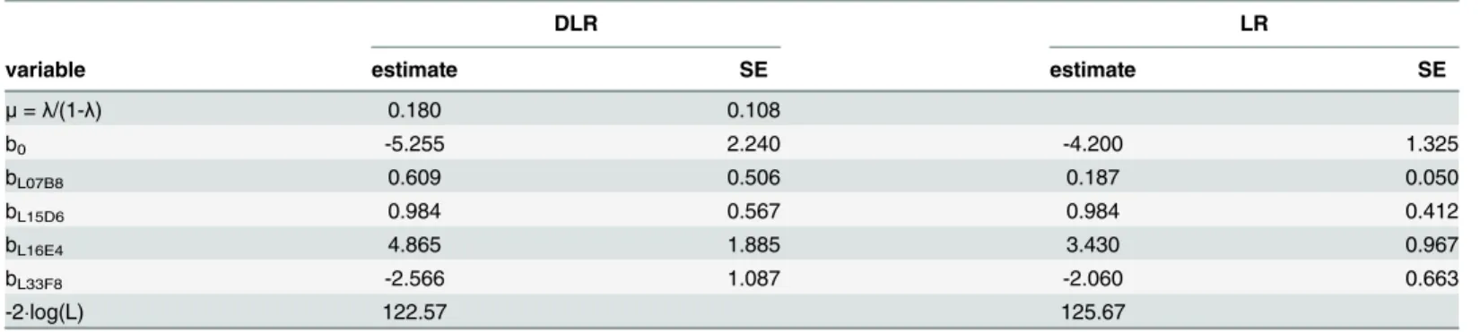
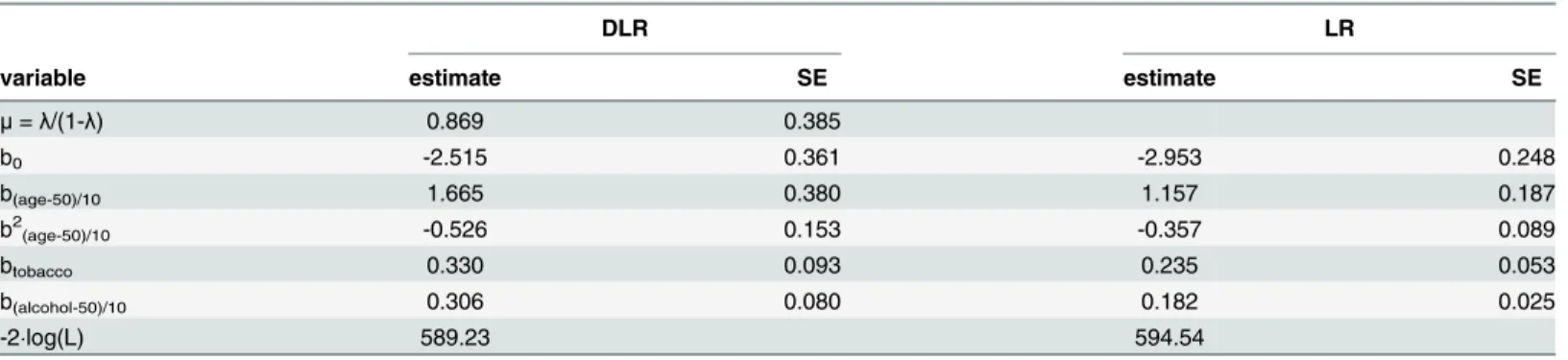
he multiple logistic regression model using hospital mortality as the dependent outcome variable (to study the risk factors for death) showed that severity of illness, according

It is noteworthy that in the new Interinstitutional Agreement between the European Parliament, the Council of the European Union and the European Commission on Better Law-Making (IIA)

In the second model for this stage, see appendix I (Table - Ordered Logistic Regression II Individual Parameters), we have statistical significance for the variable level

21 Cf. HAHN, Christologüche Hoheitstitel, 141 s.. ORIGEM E EVOLUÇÃO DO MESSIANISMO EM ISRAEL 47 da esperança de Israel, tanto nas de tipo profético, como nas de tipo sapiencial

Based on these estimations, six feminine and three masculine plants were selected to perform controlled pollinations between landraces with different tuber pulp color for

Luís Onofre considers that the most direct competitors for both of his companies are the French and Italian companies and brands that operate in the footwear luxury