Thermoelastic Property of a Semi-Infinite Medium Induced by a Homogeneously
Illuminating Laser Radiation
Ibrahim A. Abdallah, Amin F. Hassany, Ismail M. Tayel
Dept. of Mathematics,yDept. of Physics, Helwan University, Helwan, 11795, Egypt
E-mail: [email protected]
The problem of thermoelasticity, based on the theory of Lord and Shulman with one relaxation time, is used to solve a boundary value problem of one dimensional semi-infinite medium heated by a laser beam having a temporal Dirac distribution. The sur-face of the medium is taken as traction free. The general solution is obtained using the Laplace transformation. Small time approximation analysis for the stresses, displace-ment and temperature are performed. The convolution theorem is applied to get the response of the system on temporally Gaussian distributed laser radiation. Results are presented graphically. Concluding that the small time approximation has not affected the finite velocity of the heat conductivity.
1 Introduction
The classical theory (uncoupled) of thermoelasticity based on the conventional heat conduction equation. The conventional heat conduction theory assumes that the thermal disturbances propagate at infinite speeds. This prediction may be suitable for most engineering applications but it is a physically unac-ceptable situation, especially at a very low temperature near absolute zero or for extremely short-time responses.
Biot [1] formulated the theory of coupled thermoelastic-ity to eliminate the shortcoming of the classical uncoupled theory. In this theory, the equation of motion is a hyperbolic partial differential equation while the equation of energy is parabolic. Thermal disturbances of a hyperbolic nature have been derived using various approaches. Most of these ap-proaches are based on the general notion of relaxing the heat flux in the classical Fourier heat conduction equation, thereby, introducing a non Fourier effect.
The first theory, known as theory of generalized thermoe-lasticity with one relaxation time, was introduced by Lord and Shulman [2] for the special case of an isotropic body. The ex-tension of this theory to include the case of anisotropic body was developed by Dhaliwal and Sherief [4].
In view of the experimental evidence available in favor of finiteness of heat propagation speed, generalized thermoelas-ticity theories are supposed to be more realistic than the con-ventional theory in dealing with practical problems involving very large heat fluxes and/or short time intervals, like those occurring in laser units and energy channels.
The purpose of the present work is to study the thermoe-lastic interaction caused by heating a homogeneous and iso-tropic thermoelastic semi-infinite body induced by a Dirac pulse having a homogeneous infinite cross-section by em-ploying the theory of thermo-elasticity with one relaxation time. The problem is solved by using the Laplace transform technique. Approximate small time analytical solutions to
stress, displacement and temperature are obtained. The con-volution theorem is applied to get the spatial and temporal temperature distribution induced by laser radiation having a temporal Gaussian distribution. At the end of this work we present the computed results obtained from the theoretical re-lations applied on a Cu target.
2 Formulation of the problem
We consider a thermoelastic, homogeneous, isotropic semi-infinite target occupying the regionz > 0, and initially at uniform temperature T0. The surface of the target z = 0 is heated homogeneously by a leaser beam and assumed to be traction free. The Cartesian coordinates(x; y; z)are con-sidered in the solution andz-axis pointing vertically into the medium. The equation of motion in the absence of the body forces has the form
ji;j = ui; (1)
whereij is the components of stress tensor,uiis the com-ponents of displacement vector and is the mass density. Due to the Lord and Shalman theory of coupled thermoelas-ticity [2] (L-S) who considered a wave-type heat equation by postulating a new law of heat conduction equation to replace the Fourier’s law
cE
@T
@t + t0 @2T
@t2
+
+ T0div
@u
@t + t0 @2u
@t2
= k r2T ; (2)
whereT0is a uniform reference temperature,=(3+2)t,
, andare Lame’s constants.tis the linear thermal expan-sion coefficient,cEis the specific heat at constant strain and
kis the thermal conductivity. The boundary conditions:
kdTdz = A0q0(t) ; z = 0 ; (4)
whereA0is an absorption coefficient of the material,q0is the intensity of the laser beam and(t)is the Dirac delta function [5]. The initial conditions:
T (z; 0) = T0
@T @t =
@2T
@t2 =
@w @t =
@2w
@t2 = 0 ; at t = 0 ; 8 z
9 > = > ;: (5)
Due to the symmetry of the problem and the external ap-plied thermal field, the displacement vectoruhas the compo-nents:
ux= 0 ; uy= 0 ; uz= w(z; t) : (6)
From equation (6) the strain componentseij, and the re-lation of the strain components to the displacement read;
exx= eyy= exy= exz= eyz = 0
ezz=@w@z
eij= 12(ui;j+ uj;i)
9 > > > > > = > > > > > ;
: (7)
The volume dilationetakes the form
e = exx+ eyy+ ezz= @w@z : (8)
The stress components are given by:
xx= e (T T0)
yy= e (T T0)
zz= 2@w@z + e (T T0)
9 > > > > = > > > > ;
; (9)
where
xy= 0
xz = 0
yz = 0
9 > = >
;: (10)
The equation of motion (1) will be reduces to
zz;z+ xz;x+ yz;y = uz: (11)
Substituting from (9) and (10) into the last equation and using = T T0we get,
(2 + )@@z2w2 @z@ = @@t2w2 ; (12)
whereis the temperature change above a reference temper-atureT0. Differentiating (12) with respect tozand using (8), we obtain
(2 + )@@z2e2 @z@22 = @@t22e: (13)
The energy equation can be written in the form:
@ @t + t0
@2
@t2
(cE + T0e) = kr2T
r2 @2
@z2
9 > > = > > ;:
(14)
For convenience, the following non-dimensional quanti-ties are introduced
z= c
1z ; w= c1w ; t= c21 t
t
0= c21 t0; ij= ij ; = TT T0 0
= ckE; c2
1= ij = + 2
9 > > > > > = > > > > > ;
: (15)
Substituting from (15) into (12) we get after dropping the asterisks and adopting straight forward manipulation
r2e g
1r2 = @ 2e
@t2
r2 =@
@t + t0 @2e
@t2
( + g2e)
9 > > = > > ;;
(16)
whereg1=(2+)T0 andg2= cE. Substituting from (15) into (9) we get,
xx= yy= e 1
zz= e 1
)
; (17)
where = (2+) , = and 1= T0. We now intro-duce the Laplace transform defined by the formula:
f(z; s) =
Z 1
0 e
stf(z; t)dt : (18)
Applying (18) to both sides of equation (16) we get,
(r2 s2) e g
1r2 = 0 ; (19)
(r2 s(1 + t
0s)) s(1 + t0s) g2e = 0 : (20) Eliminating andebetween equation (19) and (20) we get the following fourth-order differential equations satisfied byeand; respectively
(r4 Ar2+ C) e = 0 ; (21)
(r4 Ar2+ C) = 0 ; (22)
withA = s2+s(1+t0s)(1+g1g2)andC = s3(1+t0s). One can solve these fourth order ordinary differential equations by usinge kzand finding the roots of the inditial equation
suppose thatki (i = 1; 2) are the positive roots, then the so-lution of (23) forz>0andki> 0are; respectively
e(z; s) =
2
X
i=1
Aie kiz (24)
and
(z; s) =X2
i=1
A0ie kiz; (25)
whereAi = Ai(s)and A0i = A0i(s) are some parameters depending only onsandki are functions ofs. Substituting by (24) and (25) into (20) we get the relation,
A0i = s(1 + t0s)g2 k2
i s(1 + t0s)Ai; (26)
while Laplace transform of Equation (8) and integration w.r.t.
zwe obtain
w(z; s) = X2
i=1
Ai
ki e
kiz: (27)
Substituting from Equation (24) and Equation (26) into (17) we get the stresses,
xx= yy= 2
X
i=1
Aie kiz
(k2i s(1 + t0s)) s(1 + t0s)1g2
k2
i s(1 + t0s) :
(28)
zz= 2
X
i=1
Aie kiz
(k2i s(1 + t0s)) s(1 + t0s)1g2
k2
i s(1 + t0s) :
(29)
Therefore it is easy to determineAiandA0ifori = 1; 2
A1= A0q0(k 2
1 s(1 + t0s))B1(s)
g2s(1 + t0s)[ k1B2(s) + k2B3(s)]; (30)
A2= A0q0(k 2
2 s(1 + t0s))B1(s)
g2s(1 + t0s)[ k1B2(s) + k2B3(s)]; (31)
A01= A0q0B1(s)
[ k1B2(s) + k2B3(s)]; (32)
A02=[ k A0q0B1(s)
1B2(s) + k2B3(s)]; (33)
where B1(s) = (k22 s(1 + t0s))( + 1g2), B2(s) =
= k2
2 s(1 + t0s)( + 1g2), and also B3(s) = k21
s(1 + t0s)( + 1g2).
3 Small time approximation
We now determine inverse transforms for the case of small values of time (large values ofs). This method was used by
Hetnarski [6] to obtain the fundamental solution for the cou-pled thermelasticity problem and by Sherief [7] to obtain the fundamental solution for generalized thermoelasticity with two relaxation times for point source of heat. k1 andk2are the positive roots of the characteristic equation (23), given by
k1=
s 2 h
s + (1 + t0s)(1 + ) +
+ps2+2s( 1)(1+t0s)+(1+t0s)2(1+)2i
1 2
;
(34)
k2=
s 2 h
s + (1 + t0s)(1 + ) +
p
s2+2s( 1)(1+t0s)+(1+t0s)2(1+)2i
1 2
;
(35)
where = g1g2=2t(3 + 2)2T0
cE(2 + ) . Setting v =
1
s, equations
(34) and (35) can be expressed in the following from
ki= v 1[fi(v)]12; i = 1; 2 ; (36) where
f1(v) = 12
h
1 + (v + t0)(1 + ) +
+p1 + 2( 1)(v + t0) + (v + t0)2(1 + )2
i
; (37)
f2(v) = 12
h
1 + (v + t0)(1 + )
p
1 + 2( 1)(v + t0) + (v + t0)2(1 + )2
i
: (38)
Expanding f1(v) and f2(v) in the Maclaurin series aroundv = 0and consider only the first four terms, can be writtenfi(v)(i = 1; 2) as
fi(v) = ai0+ ai1v + ai2v2+ ai3v3; i = 1; 2 ; (39) where the coefficients of the first four terms are given by
a10=1+(1+) t0+
p
1+2( 1) t0+(1+)2t20
2 a20=1+(1+) t0
p
1+2( 1) t0+(1+)2t20
2
a11=12
"
(1+) p( 1) t0+(1+)2t0 1+2( 1)t0+(1+)2t20
#
a21=12
"
(1+)+p( 1) t0+(1+)2t0 1+2( 1) t0+(1+)2t20
#
a12=
[1+2( 1) t0+(1+)2t20]32
a22=
[1+2( 1) t0+(1+)2t20]32
a13= ( 1++(1+) 2t
0)
[1+2( 1)t0+(1+)2t20]32
a23= ( 1++(1+) 2t0)
[1+2( 1)t0+(1+)2t20]
3 2
9 > > > > > > > > > > > > > > > > > > > > > > > > > > > > > > > > = > > > > > > > > > > > > > > > > > > > > > > > > > > > > > > > > ;
Next, we expand[fi(v)]
1
2in the Maclaurin series around
v = 0and retaining the first three terms, we obtain finally the expressions fork1andk2which can be written in the form
ki= v 1 bi0+ bi1v + bi2v2; i = 1; 2 ; (41)
where
bi0= pai0;
bi1= 2pai1a i0 ;
and
bi2= 1
8a32
i0(9ai2ai0 a2i0)
:
Considerkito be written as
ki= bi0s + bi1; i = 1; 2 : (42)
Applying Maclaurin series expansion aroundv = 0of the following expressions;
1 kiAi;
s(1 + t0s)g2
k2
i s(1 + t0s)Ai;
(k2
i s(1 + t0s)) s(1 + t0s)1g2
k2
i s(1 + t0s)
Ai;
(k2
i s(1 + t0s)) s(1 + t0s)1g2
k2
i s(1 + t0s)
Ai;
i = 1; 2 :
We find that,w,xx,yy, andzzcan be written in the following form
=c0
s + c1
s2 +
c2
s3
e k1z+
+c3 s +
c4
s2 +
c5
s3
e k2z;
(43)
w =csw02 +csw13 +csw24 e k1z+
+cw3 s2 +
cw4
s3 +
cw5
s4
e k2z;
(44)
xx = yy=c0s +cs12 +cs23
e k1z+
+c3s +cs42 +cs53 e k2z;
(45)
zz=cz0s +csz12 +csz23
e k1z+
+cz3s +csz42 +csz53e k2z;
(46)
where
c0=yf1
0=0:00002466
c1=yf2 0
f1y1
f2
0 =0:000666
c2=yf3 0+
f2 1y1
f3 0
f2y1+f1y2
f2
0 = 0:911471
c3=y 1
f0=0:705
c4=y 2
f0
f1y1
f2
0 = 1:7696
c5=y 3
f0+
f2 1y1
f3 0
f2y1+f1y2
f2
0 =50:6493
cw0=AR1
0= 0:0007519
cw1= RR1A21
0 +
A2
R0=0:18
cw2=R 2 1A1
R3 0
R2A1+R1A1
R2
0 +
A3
R0=26:90
cw3=A 1
R0=0:000106
cw4= R 1A1
R2
0 +
A 2
R
0= 0:000493
cw5=R 2 1 A1
R3 0
R
2A1+R1A1
R2 0 + A 3 R 0=194:0138
c0=x1
1=0:001511
c1=x2 1
2x1
2
1 = 0:03623
c2=x1 1
2x2
2 1
x13
2
1 = 54:064
c3=x 1
1= 0:002985
c4=x 2
1
2x1
2
1 =0:07314
c5=x 1
1
2x2
2 1
x 13
2
1 =53:02
cz0=L1
1=0:003015
cz1=L2 1
2L1
2
1 = 0:0722
cz2=L1 1
2L2
2 1
L13
2
1 = 107:88
cz3=L 1
1= 0:003
cz4=L 2
1
2L1
2
1 =0:0722
cz5=L 1
1
2L2
2 1
L 13
From equation (39), we obtain
e k1z= e (b10s+b11)z = e b11ze b10sz;
and
e k2z= e (b20s+b21)z = e b21ze b20sz:
Applying the inverse Laplace transform for equations (43, 44, 45, 46) we get,w,xx,yy andzz in the fol-lowing form
= e b11z
1H(t b10z) + e b21z2H(t b20z) ; (48)
where
1=
h
c0+ c1(t b10z) +c22(t b10z)2
i ;
2=
h
c3+ c4(t b20z) +c25(t b20z)2
i ;
and also
w = e b11zW
1H(t b10z) + e b21zW2H(t b20z) ; (49)
where
W1=
cw0(t b10z)+cw1(t b10z) 2
2 +
cw2(t b10z)3
6
;
W2=
cw3(t b20z)+cw4(t b20z) 2
2 +
cw5(t b20z)3
6
;
and also
xx= yy =
= e b11z
1H(t b10z) + e b21z2H(t b20z) ;
(50)
where
1=
c0+ c1(t b10z) + c2(t b10z) 2
2
;
2=
c3+ c4(t b20z) + c5(t b20z) 2
2
;
and also
zz= e b11zZ1H(t b10z) + e b21zZ2H(t b20z) ; (51)
where
Z1=
cz0+ cz1(t b10z) + cz2(t b10z) 2
2
;
Z2=
cz3+ cz4(t b20z) + cz5(t b20z) 2
2
;
andH(t bi0z)is Heaviside’s unit step functions. By us-ing the convolution theoremh(t) = R0tf()g(t )d for (48), (49), (50) and (51) we obtain under the assumption that
f() = e (tb )2'2 ; which represents the time behavior of the
intensity of the laser radiation, wheretbis the time at which
f()has maximum. Here'is the time at which the intensity of the laser radiation reduces to1e
= e b11z
c0+c1(t b10z)+c2(t b10z) 2
2 +
+ c2(t b10z) 2
2 + '
2c 2 4
p 2 'erf
t
'
c2t'4e t2 '2+
+ (c1+c2(t b10z)) ' 2 2
1 e '2t2
+
+ e b21z
c3+c4(t b10z)+c5(t b10z) 2
2 +
+ '24c5
p 2 'erf
t
'
c2t'4e t2 '2+
+ (c4+c5(t b10z)) ' 2 2
1 e '2t2
;
(52)
w = e b11z
cw0(t b10z)+ cw12
(t b10z)2+ ' 2 2
+
+ cw2
(t b10z)3
6 + '
2 4
p 2 'erf
t
'
cw0+cw1(t b10z) ' 2c
w2 12
'2 (t2 '2)e '2t2+
+ cw22 (t b10z)2
'2 2
1 e '2t2
1
4(cw1+cw2(t b10z))t'2e
t2 '2
+
+ e b21z
cw3(t b20z)+ cw42
(t b10z)2+ ' 2 2
+
+ cw5
(t b10z)3
6 + '
2 4
p 2 'erf
t
'
cw3+cw4(t b10z) ' 2c
w5 12
'2 (t2 '2)e '2t2+
+ cw52 (t b10z)2
'2 2
1 e '2t2
1
4(cw4+cw5(t b10z))t'2e
t2 '2
;
(53)
zz= e b11z
cz0+cz1(t b10z)+ cz22 (t b10z)2+
+ '24cz2
p 2 'erf
t
'
c
z2 4 t'e
t2 '2+
+ (cz1+cz2(t b10z)
'2 2
1 e '2t2
+
+ e b11z
cz3+cz4(t b10z)+ cz52 (t b10z)2+
+ '2cz5 4
p 2 'erf
t
'
c
z5 4 t'e
t2 '2+
+ (cz4+cz5(t b10z)) ' 2 2
1 e '2t2
;
xx= yy= e b11z
c0+c1(t b10z) +
+ c22 (t b10z)2+ ' 2c
2 4
p 2 'erf
t
'
c
2' 4 te
t2 '2+
+ (c1+c2(t b10z)) ' 2 2
1 e '2t2
+
+ e b21z
c3+c4(t b20z)+ c52 ((t b10z)2+
+ c54'2
' p
2 erf
t
'
'c
5 4 te
t2 '2+
+ (c4+c5(t b10z)) ' 2 2
1 e '2t2
:
(55)
4 Computation and discussions
We have calculated the spatial temperature, displacement and stress,w, xx, yy andzz with the time as a parameter for a heated target with a spatial homogeneous laser radia-tion having a temporally Gaussian distributed intensity with a width of (10E-3 s). We have performed the computation for the physical parametersT0= 293K, = 8954Kg/m3,
A = 0:01; cE= 383:1J/kgK;
' = 10 3s; = g
1g2= 0:01680089;
t= 1:78(10 5)K 1; k = 386W/mK;
= 7:76(1010)kg/m sec2; = 3:86(10)10kg/m sec2
and
t0= 0:02sec
for Cu as a target. We obtain the results displayed in the fol-lowing figures.
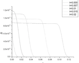
Considering surface absorption the obtained results in Figure 1 show the temperature, Figure 2 display the tem-poral temperature distribution and the temtem-poral behavior of the laser radiation, Figure 3 for the displacementw, Figure 4 for the stresszzand Figure 5 for the stressesxxandyy.
The coupled system of differential equations describing the thermoelasticity treated through the Laplace transform of a temporally Dirac distributed laser radiation illuminating ho-mogeneous a semi-infinite target and absorbed at its irradi-ated surface. Since the system is linear the response of the system on the Dirac function was convoluted with a tem-porally Gaussian distributed laser radiation. The theoretical obtained results were applied on the Cu target. Figure 1 il-lustrates the calculated spatial distribution of the temperature per unit intensity at different values of the time parameter
(t = 0:005; 0:007; 0:01; 0:015;and0:02). From the curves it is evident that the temperature has a finite velocity expressed through the strong gradient of the temperature which moves deeper in the target as the time increases.
Fig. 1: The temperature distribution per unit intensity versusz with the time as a parameter.
Fig. 2: (A) The temporal temperature distributionper unit inten-sity form the. (B) The temporal behavior of the laser radiation which is assumed to have a Gaussian distribution with width' = 10 3s.
Figure 2 represent the calculated front temporal tempera-ture distribution per unit intensity (curve A); as a result of the temporal behavior of the laser radiation which is assumed to have a Gaussian distribution with a width equals to (10E-3 s) (curve B). From the figure it is evident that the temperature firstly increases with increasing the time this can be attributed to the increased absorbed energy which over compensates the heat losses given by the heat conductivity inside the material. As the absorbed power equals the conducted one inside the material the temperature attains its maximum value. the max-imum of the temperature occurs at later time than the maxi-mum of the radiation this is the result of the heat conductivity of Cu and the relatively small gradient of the temperature in the vicinity ofz = 0as seen from Figure 1. After the ra-diation becomes week enough such that it can not compen-sate the diffused power inside the material the temperature decreases monotonically with increasing time.
Fig. 3: The displacement distributionuper unit intensity versusz with the time as a parameter.
Fig. 4: The stresszz distribution per unit intensity versuszwith the time as a parameter.
displacement increases monotonically with time. It attains smaller gradient with increasing z. Both effects can be at-tributed to the temperature behavior. The negative displace-ment results from the co-ordinate system which is located at the front surface with positive direction of thez-axis pointing down words.
Figure 4 illustrates the spatial distribution of stress zz
per unit intensity at the times (0.01, 0.015 and 0.02). Since,
zz= e 1, thus from Figure 3zzattains maxima at the
locations for which the gradient of the displacement exhibits maxima and this is practically at the same points for which
zzis maximum. The calculations showed thatxx andyy
have the same behavior aszz.
5 Results and conclusions
The thermoelasticity problem formulated by a coupled linear system of partial differential equations was discussed. The system was decoupled to provide a fourth order linear diff er-ential equations which were solved analytically using Laplace
Fig. 5: The stress distributionxxandyyper unit intensity versus zwith the time as a parameter.
transform. The small time approximation analysis was per-formed for the solution of temperature, displacement and for the stresses; showing that the finite velocity of the temper-ature described by the D.Es system was not affected by the small time approximation.
Acknowledgements
The authors want to thanks Dr. Ezzat F. Honin for his valu-able discussions and comments.
Submitted on June 25, 2008/Accepted on August 15, 2008
References
1. Biot M. Thermoelasticity and irreversible thermo-dynamics.J. Appl. Phys., 1956, v. 27, 240–253.
2. Lord H. and Shulman Y. A generalized dynamical theory of thermoelasticity.J. Mech. Phys. Solid., 1967, v. 15, 299–309.
3. Bondi H. Negative mass in General Relativity.Review of Mod-ern Physics, 1957, v. 29 (3), 423–428.
4. Dhaliwal R. and Sherief H. Generalized thermoelasticity for anisotropic media.Quatr. Appl. Math., 1980, v. 33, 1–8.
5. Hassan A.F., El-Nicklawy M.M., El-Adawi M.K., Nasr E.M., Hemida A.A. and Abd El-Ghaffar O.A. Heating effects induced by a pulsed laser in a semi-infinite target in view of the theory of linear systems.Optics&Laser Technology, 1996, v. 28 (5), 337–343.
6. Hetnarski R. Coupled one-dimensional thermal shock problem for small times.Arch. Mech. Stosow., 1961, v. 13, 295–306.