Laplacian Estrada and normalized Laplacian Estrada indices of evolving graphs.

Laplacian Estrada and Normalized Laplacian

Estrada Indices of Evolving Graphs

Yilun Shang1*

1Department of Mathematics, Tongji University, Shanghai, China

*shyl@tongji.edu.cn

Abstract

Large-scale time-evolving networks have been generated by many natural and technologi-cal applications, posing challenges for computation and modeling. Thus, it is of theoretitechnologi-cal and practical significance to probe mathematical tools tailored for evolving networks. In this paper, on top of the dynamic Estrada index, we study the dynamic Laplacian Estrada index and the dynamic normalized Laplacian Estrada index of evolving graphs. Using linear alge-bra techniques, we established general upper and lower bounds for these graph-spectrum-based invariants through a couple of intuitive graph-theoretic measures, including the num-ber of vertices or edges. Synthetic random evolving small-world networks are employed to show the relevance of the proposed dynamic Estrada indices. It is found that neither the static snapshot graphs nor the aggregated graph can approximate the evolving graph itself, indicating the fundamental difference between the static and dynamic Estrada indices.

Introduction

With the development of modern digital technologies, time-dependent complex networks arise naturally in a variety of areas from peer-to-peer telecommunication to online human social be-havior to neuroscience. The edges in these networks, which represent the interactions between elements of the systems, change over time, posing new challenges for modeling and computa-tion [1,2]. Basically, the time ordering of the networks (or graphs) induces an asymmetry in terms of information communication, even though each static snapshot network is symmetric, i.e., undirected [3]. For example, ifucommunicates withv, and then latervcommunicates withw, the information fromucan reachwbut not vice versa.

The Estrada index as a graph-spectrum-based invariant, on the other hand, was put forward by Estrada [4], initially for static graphs. Since its invention in 2000, the Estrada index has found a range of applications in chemistry and physics, including the degree of folding of long-chain polymeric molecules (especially proteins) [4,5], extended atomic branching [6], and vi-brations in complex networks [7–10], etc. The Estrada index of a graphGwithnvertices is de-fined as [11]

EEðGÞ ¼X

n

i¼1

eli_{; ð1Þ}

a11111

OPEN ACCESS

Citation:Shang Y (2015) Laplacian Estrada and Normalized Laplacian Estrada Indices of Evolving Graphs. PLoS ONE 10(3): e0123426. doi:10.1371/ journal.pone.0123426

Academic Editor:Yongtang Shi, Nankai University, CHINA

Received:January 12, 2015

Accepted:March 3, 2015

Published:March 30, 2015

Copyright:© 2015 Yilun Shang. This is an open access article distributed under the terms of the Creative Commons Attribution License, which permits unrestricted use, distribution, and reproduction in any medium, provided the original author and source are credited.

Data Availability Statement:All relevant data are within the paper.

Funding:This study is partly supported by Program for Young Excellent Talents in Tongji University under Grant No. 2014KJ036. The funders had no role in study design, data collection and analysis, decision to publish, or preparation of the manuscript.

whereλ1,λ2, ,λnare the eigenvalues of the adjacency matrix ofG. Numerous mathematical

results for the Estrada index have been obtained, especially the upper and lower bounds. For these results, we refer the reader to an updated review [12] and the references therein. From the combinatorial construction, it is easy to see thatEE(G) counts the weighted sum of closed walks of all lengths inG. The Estrada index—viewed as a redundancy measure of alternative

paths—is shown to be instrumental in gauging robustness of networks [9,13–17].

However, all the above mentioned works on the Estrada index are only confined to static graphs, which is a drawback from the perspective of network science [2]. Very recently, the Es-trada index of time-dependent networks is introduced in [18] based on a natural definition of a walk on an evolving graph, namely, a time-ordered sequence of graphs over a fixed vertex set. Given an evolving graph, this dynamic Estrada index respects the time-dependency and gener-alizes the (static) Estrada index, conveniently summarizing those networks. Some basic proper-ties and lower and upper bounds for the dynamic Estrada index are also developed in [18].

In the present paper, we go deeper in this direction and consider the dynamic Laplacian Es-trada index and the dynamic normalized Laplacian EsEs-trada index. In addition to the spectrum of adjacency matrix, the spectral theory of (normalized) Laplacian matrix is another well devel-oped part in algebraic graph theory [19,20]. We show that it is possible to define dynamic (normalized) Laplacian Estrada index in full analogy with dynamic Estrada index [18]. In fact, the static Laplacian Estrada and normalized Laplacian Estrada indices have already been pro-posed in [21] and [22], respectively. As such, our work can be viewed as an extension from stat-ic case to dynamstat-ic case. The gap between them, nevertheless, is non-trivial as described at the outset.

After giving the two dynamic indices and some basic properties, we establish refined upper and lower bounds for them, respectively. All these bounds are presented in terms of the several simplest graph-theoretic parameters, such as the numbers of vertices (or nodes) and edges, and the maximum and minimum degrees, offering both conceptual and computational advantages. Moreover, the similarity and difference between dynamic Estrada index and dynamic (normal-ized) Laplacian Estrada index are explored. In some cases, the dynamic (normal(normal-ized) Laplacian Estrada index behaves better than its counterpart due to the nice properties of Laplacian spec-trum [20].

Next, we use synthetic examples (random evolving small-world networks) to validate the relevance of our proposed various dynamic Estrada indices. Simulation results highlight the fundamental difference between the static and dynamic Estrada indices—in general, neither

the static snapshot graphs nor the aggregated/summarized graph approximates the evolving graph itself.

We mention here that there is an increasing interest in studying evolving graphs in recent few years. The most conceptually relevant works are [3,23–25], where static Katz-like centrali-ties and network communicability are accommodated to address the time-evolving scenarios. A continuous-time dynamical systems view of node centrality in evolving networks is provided in [26]. However, these works are mostly concerned about algorithmic aspects, such as compu-tational cost, efficiency and storage. We also note that the evolving networks have found a place in the analysis of coevolutionary games and more broadly, the emergence of cooperation in complex adaptive systems [27–29].

Results

Concepts of dynamic Estrada indices

LetGbe a simple graph withnvertices. Denote byA=A(G) the adjacency matrix ofG, and λ₁(A),λ₂(A), ,λ_n(A) the eigenvalues ofA. SinceAis a real symmetric matrix, we assume that the eigenvalues are labeled in a non-increasing manner asλ1(A)λ2(A) λn(A).

Let tr() represent the trace of a matrix. Fork= 0, 1, , defineMkðAÞ ¼ Pn

i¼1l k

iðAÞthekth spectral moment of the adjacency matrix. It follows from (1) that the Estrada index ofGcan be written as

EEðGÞ ¼X

n

i¼1

eliðAÞ_¼X 1

k¼0

MkðAÞ

k! ¼ X1

k¼0 trðAk_Þ

k! ¼trðe A_Þ;

ð2Þ

where the power-series expansion of matrix exponentialeAis employed:

eA_¼IþAþA 2

2!þ þ

Ak

k!þ ¼

X1

k¼0

Ak

k! ð3Þ

withIbeing then-dimensional identity matrix. An extension to weighted graphs can be found in [30].

Suppose we have an evolving graph, namely, a time-ordered sequence of simple graphsG1,

G2, ,GNover a fixed setVofnvertices, at the time points 1, 2, ,N. LetAt=A(Gt) be the

adjacency matrix for the snapshot graphGtfort= 1, 2, ,N. Letmtdenote the number of

edges ofGtandλ1(At)λ2(At) λn(At) the eigenvalues ofAt.

Definition 1. [18] The Estrada index of an evolving graphG1,G2, ,GNis defined as

EEðG1;G2; ;GNÞ ¼trðe

A1_eA2 _eANÞ: ð₄Þ

The following concept of dynamic walk in an evolving graph is introduced in [3].

Definition 2. A dynamic walk of lengthkfrom vertexv12Vto vertexvk+12Vconsists of a

sequence of edges {v1,v2}, {v2,v3}, , {vk,vk+1} and a non-decreasing sequence of time points

1t1t2 tkNsuch that the (vi,vi+1) element ofAti, (Ati)vi,vi+16¼0 for 1ik.

In the light of (3), the product of matrix exponentialseAt1eAt2 eAtkis equal to the summa-tion of all products of the form

1

Z1!Z2! Zk!

AZ1 t1A

Z2 t2 A

Zk

tk ¼

1

Z1!Z2! Zk!

Ad1 ts1A

d2 ts2 A

dr

t_sr;

wherets1<ts2< <tsrare all the distinct values in the time sequencet1t2 tk, and

the multiplicity oftsiisδi, namely,δi=∑tj=tsiηj, 1ir. Note that the matrix productAt1At2

Atkhas (vp,vq) element that counts the number of dynamic walks of lengthkfromvptovq

on which theith step of the walk takes place at timeti, 1ik. Thus, by setting

‘≔Pri¼1di¼ Pk

j¼1Zj, we observe that the dynamic Estrada index (4) is a weighted sum of the numbers of closed dynamic walks of all lengths, where the number of walks of lengthℓ_(withδ i

edges followed at timetsi, 1ir) is penalized by a factor

1

Z1!Z2!Zk!, naturally extending the

(static) Estrada index (2).

Dynamic Laplacian Estrada index. Given a simplen-vertex graphG, its degree matrixD

(G) is defined as a diagonal matrix with degrees of the corresponding vertices ofGon the main diagonal and zero elsewhere. The Laplacian matrix ofGisL=L(G)≔D(G)−A(G). We as-sume thatλ₁(L)λ₂(L) λ_n(L) = 0 are the Laplacian eigenvalues ofG[20].

The Laplacian analogue of the Estrada index is defined in [21] as

LEEðGÞ ¼X

n

i¼1

An essentially equivalent definition can be found in [31]. We refer the reader to [32–34] for re-cent results ofLEE(G) and its variants. Fork= 0, 1, , defineMkðLÞ ¼

Pn i¼1l

k

iðLÞthekth spectral moment of the Laplacian matrix. Then, the expression (5), in parallel with (2), implies that

LEEðGÞ ¼X

n

i¼1

eliðLÞ_¼X 1

k¼0

MkðLÞ

k! ¼ X1

k¼0 trðLk_Þ

k! ¼trðe L_Þ;

which elicits the following dynamic Laplacian Estrada index:

Definition 3. The Laplacian Estrada index of an evolving graphG1,G2, ,GNis defined as

LEEðG1;G2; ;GNÞ ¼trðeL1eL2 eLNÞ; ð6Þ whereLt=L(Gt),t= 1, 2, ,N.

For two simple graphsGandHover the same vertex setV, we define their weighted union as an edge-weighted graphGtHwith adjacency matrix (A(GtH))u,v= 2 if {u,v} appears in

bothGandH, and (A(GtH))u,v= 1 if {u,v} appears in just one ofGandH. For an integer

N>0, letGðNÞ

≔GtG tG

|fflfflfflfflfflfflfflfflfflffl{zfflfflfflfflfflfflfflfflfflffl} N multiples

for short. Some elementary mathematical properties of the

dy-namic Laplacian Estrada index can be drawn straightforwardly:

1 Denote bySNbe the symmetric group of orderN. It follows from the cyclic property of

trace, that, forN3,

LEEðG1;G2; ;GNÞ ¼LEEðGsð1Þ;Gsð2Þ; ;GsðNÞÞ; s2SN; and that, for generalN,

LEEðG1;G2; ;GNÞ ¼LEEðGN;G1; ;GN 1Þ ¼ ¼LEEðG2;G3; ;G1Þ: This invariance under cyclic permutation also holds for the dynamic Estrada index [18]. 2 As a direct consequence of (6), ifGN¼Kn, the (edgeless) complement of complete graph

Kn, then

LEEðG1;G2; ;GNÞ ¼LEEðG1;G2; ;GN 1Þ: The same also holds for the dynamic Estrada index [18].

3 Suppose thatG1=G2= =GN. Then

LEEðG1;G2; ;GNÞ ¼LEEðG

ðNÞ

1 Þ: Similarly, we haveEEðG₁;G₂; ;_GNÞ ¼EEðGðN₁ ÞÞ. 4 IfG1=G2= =GNis anr-regular bipartite graph. Then

LEEðG1;G2; ;GNÞ ¼erNEEðG

ðNÞ

1 Þ: The property 4can be seen as follows.

LEEðG1;G2; ;GNÞ ¼ trðeNðrI A1ÞÞ ¼erNtrðe NA1Þ

¼ erN_trðeNA1Þ ¼_erNEEðGðNÞ 1 Þ;

where in the second last equality we used the fact that the eigenvalues ofA1are symmetric

Dynamic normalized Laplacian Estrada index. The normalized Laplacian matrixL₌L

(G) is defined as [19]

ðL_Þ i;j¼

1; i¼j; degGðviÞ 6¼0;

1

ffiffiffiffiffiffiffiffiffiffiffiffiffiffiffiffiffiffiffiffiffiffiffiffiffiffiffiffiffiffiffiffi degGðviÞdegGðvjÞ

q ; i6¼j;vi is adjacent to vj;

0; otherwise;

8 > > > > > > <

> > > > > > :

where degG(vi) is the degree of vertexviinG. If there is no isolated vertex inG, we haveL(G) =

D−1/2(G)L(G)D−1/2(G). Assume thatλ₁(L₎λ₂(L₎ λ_n(L_{) = 0 are the normalized}

Laplacian eigenvalues ofG.

The normalized Laplacian Estrada index is put forward in [35] as

L_{EEðGÞ ¼}X n

i¼1

el_iðL_Þ

: _ð7Þ

See also [22] for an essentially equivalent definition.L_{EE(G) has been addressed for a class of}

tree-like fractals [36]. Following the same reasoning in (2), we obtainL_{EE(G) = tr(e}L_{). In}

anal-ogy to (4) and (6), we have the following

Definition 4. The normalized Laplacian Estrada index of an evolving graphG1,G2, ,GN

is defined as

L_EEðG

1;G2; ;GNÞ ¼trðe

L₁ eL₂

eL_N

Þ; ð8Þ

whereL_t=L_{(Gt),t= 1, 2, ,N.}

The following basic properties of the dynamic normalized Laplacian Estrada index can be easily deduced.

5 ForN3,

L_EEðG

1;G2; ;GNÞ ¼LEEðGsð1Þ;Gsð2Þ; ;GsðNÞÞ; s2SN; and, for generalN,

L_EEðG

1;G2; ;GNÞ ¼LEEðGN;G1; ;GN 1Þ ¼ ¼LEEðG2;G3; ;G1Þ:

6 IfGN¼Kn,

L_{EEðG1;G2; ;G}

NÞ ¼LEEðG1;G2; ;GN 1Þ:

7 Suppose thatG1=G2= =GN. Then

L_EEðG

1;G2; ;GNÞ ¼ Xn

i¼1

eNliðL1Þ_;

whereasL_EEðGðNÞ

1 Þ ¼LEEðG1Þ.

8 IfG1=G2= =GNis anr-regular bipartite graph (r1). Then

L_{EEðG1;G2; ;GNÞ<e}N_EE1=r_ðG

1;G2; ;GNÞ ¼eNEE 1=r_ðGðNÞ

To see 8, we have

L_EEðG

1;G2; ;GNÞ ¼ trðeN

L₁

Þ ¼X

n

i¼1

eNðr liðA1ÞÞ=r_¼eNX n

i¼1

ðe NliðA1Þ_Þ1=r

eN X

n

i¼1

e Nl_iðA1Þ !1=r

¼ eN_tr1=r_ðeNA1_{Þ ¼e}N_EE1=r_ðGðNÞ 1 Þ;

where the equality is attained if and only ifλ₂(L_{1) = =}λ_n(L_{1) = 0. This condition is}

equiva-lent toG1 ¼KnorG1 ¼K2[Kn 2, which contradicts the assumption. Theorem 3.4 in [35] can be reproduced by settingN= 1.

Bounds for dynamic Laplacian Estrada index

Proposition 1.Let G1,G2, ,GNbe an evolving graph over a set V of size n. Then

(i) LEE_ðG_1;G_{2; ;}G_NÞ QN

t_¼1LEEðGð

N_Þ

t Þ

1=N

1

N

PN

t_¼1LEEðGð

N_Þ

t Þ.

The equalities are attained if and only if G1=G2= =GN.

(ii) max{LEE(G1),LEE(G2)}LEE(G1,G2)min{eλ1(L1)LEE(G2),eλ1(L2)LEE(G1)}.

The equalities are attained if and only ifG_1¼KnorG₂¼Kn.

Proof. (i) Since the matricesfeLtgN

t¼1are positive definite, it follows from the extended Bell-man inequality ([37, p. 481] or [38]) that

LEEðG1;G2; ;GNÞ ¼ trðeL1eL2 eLNÞ

Y

N

t¼1 trðeNLt_Þ

!1=N

¼ Y

N

t¼1

LEEðGðNÞ

t Þ !1=N

:

The last inequality follows from the arithmetic-geometric means inequality. Both equalities are attained if and only ifG1=G2= =GN.

(ii) Note that

LEEðG1;G2Þ ¼trðeL1eL2Þ ¼tr e

1 2L1

eL2_e

1 2L1

:

Therefore,LEE(G1,G2)e

λ_n(L

1)tr(e(L2)=LEE(G2) sinceλn(L1) = 0, andLEE(G1,G2)e

λ_1(L

1)tr

(e(L2_{) =e}λ1(L

1)LEE(G2). Sinceλi(L1) = 0 for alliis equivalent toG1¼Kn, the above two equali-ties hold if and only ifG1¼Kn. The desired result then follows from the property 1

_.

Remark. By counting the number of closed walks, it is shown in [18, Prop. 1] that

EEðG1;G2; ;GNÞ XN

i¼1

EEðGiÞ: ð9Þ

However, this does not hold forLEEeven in the case ofN= 2. To see this, we takeG1¼Kn. Then,

Proposition 2.The Laplacian Estrada index of an evolving graph G1,G2, ,GNover a set of

n vertices with N= 2is bounded by

1

2þ

ffiffiffiffiffiffiffiffiffiffiffiffiffiffiffiffiffiffiffiffiffiffiffiffiffiffiffiffiffiffiffiffiffiffiffiffiffiffiffiffiffiffiffi 1

4þnðn 1Þe

4ðm1þm2Þ n r

LEEðG1;G2Þ n 1þ

1 2ðe

4m1_þe4m2_Þ:

The equality on the left-hand side is attained if and only if G1 ¼G2¼Kn;and the equality on

the right-hand side is attained if and only if G1¼G2¼Knor G1 ¼G2¼K2[Kn 2.

Proof.Lower bound. Based on the well-known Golden-Thompson inequality (see e.g. [38]) we obtain

LEEðG1;G2Þ ¼trðeL1eL2Þ trðeL1þL2Þ: Therefore,

LEE2

ðG1;G2Þ Xn

i¼1

el_iðL1þL2Þ !2

¼ X

n

i¼1

e2liðL1þL2Þ_þ2 X 1i<jn

eliðL1þL2Þ_eljðL1þL2Þ_:

ð10Þ

Using Proposition 1 (i), we obtain

LEEðG1;G2Þ

1

2ðLEEðG

ð2Þ

1 Þ þLEEðG

ð2Þ

2 ÞÞ ¼

1 2

Xn

i¼1

ðe2liðL1Þ_þe2liðL2Þ_Þ

X

n

i¼1

e2l_iðLðG1tG2ÞÞ_¼X

1

k¼0 Xn

i¼1

ð2l_iðLðG1tG2ÞÞÞ k

k!

¼ nþ4ðm1þm2Þ þ

X1

k¼2 Xn

i¼1

ð2l_iðLðG1tG2ÞÞÞ k

k! ;

where the second inequality comes from the interlacing theorem in which the equality holds if and only ifG1 ¼G2 ¼Kn. Note thatL1+L2=L(G1tG2). Then,

Xn

i¼1

e2liðL1þL2Þ _¼ X n

i¼1 X1

k¼0

ð2l_iðLðG1tG2ÞÞÞ k

k!

¼ nþ4ðm1þm2Þ þ

X1

k¼2 Xn

i¼1

ð2l_iðLðG1tG2ÞÞÞ k

k!

nþ4_ðm1þm2Þ þLEEðG1;G2Þ n 4ðm1þm2Þ

¼ LEEðG1;G2Þ:

ð11Þ

On the other hand, the arithmetic-geometric means inequality yields

2 X

1i<jn

eliðL1þL2Þ_eljðL1þL2Þ _{nðn 1Þ} Y 1i<jn

eliðLðG1tG2ÞÞ_eljðLðG1tG2ÞÞ

! ₂

nðn 1Þ

¼nðn 1_Þ Y

n

i¼1

el_iðLðG1tG2ÞÞ

!n 1! 2

nðn 1Þ

¼nðn 1_Þe 4ðm1þm2Þ

Combining (10) with (11) and (12), we have

LEE2

ðG1;G2Þ LEEðG1;G2Þ þnðn 1Þe

4ðm1þm2Þ n :

SinceðLEEðG1;G2Þ 1 2Þ

2

1

4þnðn 1Þe 4ðm1þm2Þ

n 0, we arrive at

LEEðG1;G2Þ

1 2þ

ffiffiffiffiffiffiffiffiffiffiffiffiffiffiffiffiffiffiffiffiffiffiffiffiffiffiffiffiffiffiffiffiffiffiffiffiffiffiffiffiffiffiffi 1

4þnðn 1Þe

4ðm1þm2Þ n r

:

The equality is attained if and only ifG1 ¼G2¼Kn.

Upper bound. Since (eL1_−eL2₎2_{is a positive semi-definite matrix, we obtain}

2LEEðG1;G2Þ ¼ 2trðe L1_eL2Þ

trðe2L1_{Þ þtrðe}2L2_Þ

¼ X

n

i¼1 X1

k¼0

ð2l_iðL1ÞÞ k

k! þ Xn

i¼1 X1

k¼0

ð2l_iðL2ÞÞ k

k!

¼ nþ2X

n

i¼1

l_iðL1Þ þ2 Xn

i¼1

l2_iðL1Þ þ Xn

i¼1 X1

k¼3

ð2l_iðL1ÞÞ k

k!

þnþ2X

n

i¼1

l_{iðL2Þ þ}2X n

i¼1

l2 iðL2Þ þ

Xn

i¼1 X1

k¼3

ð2l_iðL2ÞÞ k

k!

¼ 2nþ4m1þ4m2þ2ðZgðG1Þ þ2m1Þ þ2ðZgðG2Þ þ2m2Þ

þX

1

k¼3

1

k! Xn

i¼1

ð2l_iðL1ÞÞ k

þX

1

k¼3

1

k! Xn

i¼1

ð2l_iðL2ÞÞ k

;

whereZgðGÞ≔Pni¼1deg 2

GðviÞis called thefirst Zagreb index of graphG[39]. Note thatPn_i¼1ð2liðL1ÞÞ

k

ð Pni¼12liðL1ÞÞ

¼KnorG1¼K2[Kn 2. Hence,

2LEEðG1;G2Þ 2nþ8m1þ8m2þ2ZgðG1Þ þ2ZgðG2Þ

þX

1

k¼3

1

k! Xn

i¼1

2l_iðL1Þ !k

þX

1

k¼3

1

k! Xn

i¼1

2l_iðL2Þ !k

¼ 2nþ8m1þ8m2þ2ZgðG1Þ þ2ZgðG2Þ

þX

1

k¼3

1

k!ð4m1Þ k

þX

1

k¼3

1

k!ð4m2Þ k

¼ 2nþ4m1þ4m2þe

4m1þ_e4m2 _8m2

1 8m

2

2 2

þ2_ðZgðG1Þ þZgðG2ÞÞ:

ð13Þ

Fort= 1, 2, denote byntthe number of non-isolated vertices inGt. We have

ZgðGtÞ ðnt 1Þ

Xn

i¼1

degGtðviÞ ð2mt 1Þ2mt;

with equality if and only ifGt=KnorGt¼K2[Kn 2. Consequently,

2LEEðG1;G2Þ 2nþ4

which yields the desired upper bound, in which equality is attained if and only ifG1=G2=Kn

orG1 ¼G2¼K2[Kn 2.

The previously communicated bounds forEE(G1,G2) in [18, Prop. 4] can not be attained.

Here, we get tight bounds forLEE(G1,G2) thanks to the nice properties of Laplacian

eigenval-ues. We mention that a version of the thermodynamic inequality might also be used here [40, Lem. 1]. Letδ(G) andΔ_{(G) be the minimum and maximum degrees of graphG, respectively.}

We in the following establish new tight bounds with the help of the minimum and maximum degrees.

Proposition 3.The Laplacian Estrada index of an evolving graph G1,G2, ,GNover a set V

of n vertices with N= 2is bounded by

1

2þ

ffiffiffiffiffiffiffiffiffiffiffiffiffiffiffiffiffiffiffiffiffiffiffiffiffiffiffiffiffiffiffiffiffiffiffiffiffiffiffiffiffiffiffiffiffiffiffiffiffiffiffiffiffiffiffiffiffiffiffiffiffiffiffiffiffiffiffiffiffiffiffiffiffiffiffiffiffiffiffiffiffiffiffiffiffiffiffiffiffiffiffiffiffiffiffiffiffiffiffiffiffiffiffiffiffiffiffiffiffiffiffiffiffiffiffiffiffiffiffiffiffiffiffiffiffiffiffiffiffiffiffiffiffiffiffiffiffiffiffiffiffiffiffiffiffiffi 1

4þnðn 1Þe

4ðm1þm2Þ

n þ8ðm1þm2Þ

2

n þ2nd12D12 4ðm1þm2Þðd12þD12Þ s

LEEðG1;G2Þ

n 1þ1

2ðe

4m1_þe4m2_{Þ þ2m}

1ð1þdðG1Þ þDðG1ÞÞ þ2m2ð1þdðG1Þ þDðG1ÞÞ

4m2

1 4m

2

2 ndðG1ÞDðG1Þ ndðG2ÞDðG2Þ;

whereδ_12≔δ(G1tG2)andΔ12≔Δ(G1tG2).The equalities are attained if and only if

G1 ¼G2¼Kn.

Proof.Lower bound. As in the proof of Proposition 2, we have (10) and (12). In the follow-ing, we aim to obtain a new estimate involvingδ12andΔ12for the first term on the right-hand

side of (10). We have

Xn

i¼1

e2liðL1þL2Þ _¼ X n

i¼1 X1

k¼0

ð2l_iðLðG1tG2ÞÞÞ k

k!

¼ nþ4ðm1þm2Þ þ2

Xn

i¼1

l2_iðLðG1tG2ÞÞ þ X1

k¼3 Xn

i¼1

ð2l_iðLðG1tG2ÞÞÞ k

k!

¼ nþ8_ðm1þm2Þ þ2ZgðG1tG2Þ þ X1

k¼3 Xn

i¼1

ð2l_iðLðG1tG2ÞÞÞ k

k!

nþ8_ðm1þm2Þ þ

8ðm1þm2Þ 2

n þ

X1

k¼3 Xn

i¼1

ð2l_iðLðG1tG2ÞÞÞ k

k!

ð14Þ

since

ZgðG1tG2Þ ¼ X

v2V deg2

G1tG2ðvÞ

1

n

X

v2V

degG1tG2ðvÞ !2

¼4ðm1þm2Þ 2

n

By using Proposition 1 (i), as in the proof of Proposition 2, we obtain

LEEðG1;G2Þ X1

k¼0 Xn

i¼1

ð2l_iðLðG1tG2ÞÞÞ k

k!

¼ nþ8_ðm1þm2Þ þ2ZgðG1tG2Þ þ X1

k¼3 Xn

i¼1

ð2l_iðLðG1tG2ÞÞÞ k

k!

nþ8ðm1þm2Þ þ4ðm1þm2Þðd12þD12Þ 2nd12D12

þX

1

k¼3 Xn

i¼1

ð2l_iðLðG1tG2ÞÞÞ k

k! ;

ð15Þ

where the last inequality follows from the fact

ZgðG1tG2Þ 2ðm1þm2Þðd12þD12Þ nd12D12

with equality attained if and only ifG1tG2is a regular graph. Indeed, this can be seen by

ex-panding the expression∑_v2V(degG

1tG2(v)−δ12)(degG1tG2(v)−Δ12), which is clearly non-positive.

Combining (10) with (12), (14) and (15), we obtain

LEE2

ðG1;G2Þ nþ8ðm1þm2Þ þ

8_ðm1þm2Þ 2

n þ ðLEEðG1;G2Þ n 8ðm1þm2Þ

4ðm1þm2Þðd12þD12Þ þ2nd12D12Þ þnðn 1Þe

4ðm1þm2Þ n

¼ 8ðm1þm2Þ 2

n þLEEðG1;G2Þ 4ðm1þm2Þðd12þD12Þ þ2nd12D12þnðn 1Þe

4ðm1þm2Þ n :

Therefore,

LEEðG1;G2Þ

1 2

2

8ðm1þm2Þ

2

n 4ðm1þm2Þðd12þD12Þ

þ2nd12D12þ

1

4þnðn 1Þe

4ðm1þm2Þ n

0;

ð16Þ

where the last inequality follows from the following three basic estimates:

e 4ðm1þm2Þ

n 1þ4ðm1þm2Þ

n ; D12n 1; and 2nd12D124ðm1þm2Þd12:

The desired lower bound then readily follows from (16).

Upper bound. As commented above, fort= 1, 2, we have

with equality attained if and only ifGtis a regular graph. Owing to (13), we obtain 2LEEðG1;G2Þ 2nþ4m1þ4m2þe

4m1_þe4m2 _8m2

1 8m

2

2 2

þ2ðZgðG1Þ þZgðG2ÞÞ

2nþ4m1þ4m2þe

4m1_þe4m2 _8m2

1 8m

2

2 2

þ4m1ðdðG1Þ þDðG1ÞÞ 2ndðG1ÞDðG1Þ

þ4m2ðdðG2Þ þDðG2ÞÞ 2ndðG2ÞDðG2Þ; which concludes the proof.

Remark. The bounds established in Proposition 2 and Proposition 3 are incomparable in general. In fact, for the lower bound, we note that

8ðm1þm2Þ 2

n 4ðm1þm2ÞD12; but 2nd12D124ðm1þm2Þd12; for the upper bound, we note that

2mt ð2mtÞ 2

; but 2mtðdðGtÞ þDðGtÞÞ ndðGtÞDðGtÞ; t¼1;2: We mention here that in the case ofN= 1, some researchers bound the Laplacian Estrada index by using some more complicated graph-theoretic parameters, including graph Laplacian energy [31], namely,∑_ijλ_i(L)j, and the first Zagreb index [41]. For more results on the graph energy, see e.g. [42–45]. The first Zagreb index was generalized to the zeroth-order general Randic index by Bollobás and Erdos [46], which was also useful in chemistry [47,48]. In con-trast, we only employ some of the most plain quantities to estimate the dynamic Laplacian Es-trada index since (i) they are relatively easily accessible for real-life complex networks of interest to us, and (ii) our motivation comes from the potential application in gauging robust-ness for large-scale networks [9,13,16], where computational complexity matters.

Bounds for dynamic normalized Laplacian Estrada index

The following proposition can be proved similarly as Proposition 1. Hence, we only state the result and omit its proof.

Proposition 4.Let G1,G2, ,GNbe an evolving graph over a set V of size n. Then

(i) LEE_ðG_1;G_{2; ;}GNÞ Q N t_¼1trðe

NLt

Þ

1=N

1

N

PN t_¼1trðe

NLt

Þ.

The equalities are attained if and only if G1=G2= =GN.

(ii) max{L_EE(G1),L_EE(G2)}L_{EE(G1,G2)min{e}λ1(L₁)L_EE(G2),eλ1(L₂)L_EE(G1)}.

The equalities are attained if and only ifG_1¼KnorG₂¼Kn.

Remark. The inequality (9) does not hold forL_{EEeither (even in the case ofN= 2). To see}

this, we takeG1 ¼Kn. Then,

L_EEðG

1;G2Þ ¼LEEðG2Þ<LEEðG1Þ þLEEðG2Þ:

Proposition 5.The normalized Laplacian Estrada index of an evolving graph G1,G2, ,GN

over a set of n(n2)vertices with each snapshot graph being connected and N=2 is bounded by

2e2

e4_þ1 1þne

2n n 1

<L_EEðG

1;G2Þ<e 2

ðn 1_þe2pffiffin

Proof.Lower bound. From the well-known Neumann inequality, we obtain

L_{EEðG1;G2Þ ¼trðe}L₁ eL₂

Þ X

n

i¼1

eliðL1Þ_eln iþ1ðL2Þ_:

An elementary result of the normalized Laplacian eigenvalues [19] indicates that 1eλi(L

1)

e2and 1eλi(L

2)e2for all 1in. Hence, applying an inverse of the Hölder inequality

(see [37, p. 18] or [49]) gives

L_EEðG

1;G2Þ

2e2

e4_þ1 Xn

i¼1

e2liðL1Þ !1

2

X

n

i¼1

e2liðL2Þ !1

2

: ð17Þ

By the arithmetic-geometric means inequality, we obtain

Xn

i¼1

e2liðL1Þ _{¼ 1þ}X n 1

i¼1

e2liðL1Þ

1þe2l1ðL1Þþ ðn ₂Þ Y

n 1

i¼2

e2liðL1Þ

! 1

n 2

¼ 1_þe2l1ðL1Þ_{þ ðn 2Þe}

2ðn l1ðL1ÞÞ n 2 ;

ð18Þ

where in the last equality we used the equationPn_i¼1liðL1Þ ¼nsinceG1is connected [19].

Define a functionfðxÞ≔1þ2e2xþ ðn 2Þe 2ðn xÞ

n 2 . It is easy to check thatf0ðxÞ ¼4e2x

2e2ðnn x2Þ0ifx2n ðn 2Þln2

2ðn 1Þ . Sincel1ðL1Þ _nn1

2n ðn 2Þln2

2ðn 1Þ for alln2 [19], it follows from

(18) that

Xn

i¼1

e2liðL1Þ_fðl

1ðL1ÞÞ f

n

n 1

¼1þne

2n

n 1_{: ð19Þ}

Likewise, we have

Xn

i¼1

e2liðL2Þ_1þne

2n

n 1_{: ð20Þ}

Combining these with (17) gives the desired lower bound

L_EEðG

1;G2Þ

2e2

e4_þ1 1þne

2n n 1

!

:

Moreover, note that if the equalities in (19) and (20) are attained, thenn= 2, namely,G1=

G2=K2. ButLEEðK2;K2Þ ¼e 4

þ1>2e2ð1þ2e4Þ

e4_þ1 , which means that the equality can not hold.

Upper bound. Again from the Neumann inequality, we arrive at

L_EEðG

1;G2Þ ¼ trðe

L₁ eL₂

Þ

X

n

i¼1

eliðL1Þ_eliðL2Þ

X

n

i¼1

e2liðL1Þ !1

2

X

n

i¼1

e2liðL2Þ !1

2

;

ð21Þ

Define the Randić_{index of a connected graphGasR}

1ðGÞ ¼

P

u;vadjacentdeg 1 G ðuÞdeg

1 G ðvÞ. It is elementary thatPni¼1l

2

iðLðGÞÞ ¼nþ2R 1ðGÞ; see e.g. [50]. We have

Xn

i¼1

e2liðL1Þ _{¼ e}2X n

i¼1

e2ðliðL1Þ 1Þ

e2 _n

þX

n

i¼1 X1

k¼1

2k

jl_iðL

1Þ 1j k

k!

!

¼ e2 _n

þX

1

k¼1

2k

k! Xn

i¼1

ðjl_iðL

1Þ 1j 2 Þ k 2 0 @ 1 A

e2 _n

þX

1

k¼1

2k

k! Xn

i¼1

jl_iðL

1Þ 1j 2 !k 2 0 @ 1 A

¼ e2 _n

þX

1

k¼1

2k

k!ð2R 1ðG1ÞÞ

k 2 0 @ 1 A

¼ e2 _{n 1þe}2p2ffiffiffiffiffiffiffiffiffiffiffiffiffiR 1ðG1Þ

:

ð22Þ

SinceG1is connected, we have [50]

R 1ðG1Þ

n

2dðG1Þ

n

2: ð23Þ

Thus, (22) leads to the following estimation

Xn

i¼1

e2liðL1Þ_e2_{ðn 1þe}2pffiffin_Þ:

Combining this and an analogous estimation forL_{2yields the desired upper bound by using}

(21).

Finally, we note that the equalities in (23) hold if and only ifG1is a 1-regular graph, namely,

G1 ¼K2[K2 [K2 |fflfflfflfflfflfflfflfflfflfflfflffl{zfflfflfflfflfflfflfflfflfflfflfflffl}

n=2 multiples

. But the first inequality in (22) is not tight for such choice ofG1.

There-fore, the equality in the upper bound can not be attained.

Remark. Recall thatδ(Gt) is the minimum degree ofGt. The above proof actually gives a

strong upper bound:

L_EEðG

1;G2Þ<e 2

ffiffiffiffiffiffiffiffiffiffiffiffiffiffiffiffiffiffiffiffiffiffiffiffiffiffiffiffiffiffiffi

n 1_þe2

ffiffiffiffiffiffiffiffiffiffiffiffi_n

dðG1Þ r r

ffiffiffiffiffiffiffiffiffiffiffiffiffiffiffiffiffiffiffiffiffiffiffiffiffiffiffiffiffiffiffi

n 1_þe2

ffiffiffiffiffiffiffiffiffiffiffiffi_n

dðG2Þ r r

: ð24Þ

Proposition 6.The normalized Laplacian Estrada index of an evolving graph G1,G2, ,GN

by

L_EEðG

1;G2Þ< e 2

ffiffiffiffiffiffiffiffiffiffiffiffiffiffiffiffiffiffiffiffiffiffiffiffiffiffiffiffiffiffiffiffiffiffiffiffiffiffiffiffiffiffiffiffiffiffiffiffiffiffiffiffiffiffiffiffiffiffiffiffiffiffiffiffiffiffiffiffiffiffiffiffiffiffiffiffi

e2_þe 2_þnþ1þe2

ffiffiffiffiffiffiffiffiffiffiffiffi_n

dðG1Þ r

2 ffiffiffiffiffiffiffiffiffiffiffiffi_n

d_ðG1Þ r s

ffiffiffiffiffiffiffiffiffiffiffiffiffiffiffiffiffiffiffiffiffiffiffiffiffiffiffiffiffiffiffiffiffiffiffiffiffiffiffiffiffiffiffiffiffiffiffiffiffiffiffiffiffiffiffiffiffiffiffiffiffiffiffiffiffiffiffiffiffiffiffiffiffiffiffiffi

e2_þe 2_þnþ1þe2

ffiffiffiffiffiffiffiffiffiffiffiffi_n

dðG2Þ r

2 ffiffiffiffiffiffiffiffiffiffiffiffi_n

dðG2Þ r s

:

Proof. As in the proof of Proposition 5, we have inequality (21). Now thatG1is connected, we know thatλn(L1) = 0,λ1(L1)2, and

Pn

i¼1liðL1Þ ¼n[19]. Therefore,

Xn

i¼1

e2liðL1Þ _{¼ e}2X n

i¼1

e2ðliðL1Þ 1Þ

e2 _e2

þe 2

þX

n 1

i¼2

e2ðl_iðL_1Þ 1Þ

!

e2 _e2_þe 2_þnþ2þX

n 1

i¼2 X1

k¼2

2kjl_iðL

1Þ 1j k

k!

!

e2 _e2_þe 2_þnþ2þX

1

k¼2

2k

k! Xn 1

i¼2

jl_iðL

1Þ 1j 2 !k 2 0 @ 1 A

¼ e2

e2

þe 2

þnþ2þX

1

k¼2

2k

k!ð2R 1ðG1ÞÞ

k

2

!

¼ e2

e2

þe 2

þnþ1_þe2 ffiffiffiffiffiffiffiffiffiffiffiffiffi2R 1ðG1Þ

p

2 ffiffiffiffiffiffiffiffiffiffiffiffiffiffiffiffiffiffi2R 1ðG1Þ p

:

ð25Þ

Define a functionf(x) =ex−_{x, which is non-decreasing on [0, +1). Thus, (23) and (25)}

in-dicate that

Xn

i¼1

e2liðL1Þ_e2 _e2_þe 2_þnþ1þe 2

ffiffiffiffiffiffiffiffiffiffiffiffi_n

dðG1Þ r

2 ffiffiffiffiffiffiffiffiffiffiffiffi

n d_ðG1Þ

r !

:

An analogous estimate forG2also holds. Combining these with (21) yields the desired

upper bound.

Finally, note that the second equality is attained in (25) if and only ifλ₁(L_{1) = 0, which is}

equivalent toG1¼Kn. However, this contradicts the assumption thatG1is connected.

There-fore, the equality in the upper bound can not be attained. The proof is complete.

Remark. It is direct to check that if

2_þe2

þe 2_<2 ffiffiffiffiffiffiffiffiffiffiffiffi_n

d_ðG1Þ r

and 2_þe2

þe 2 _<2 ffiffiffiffiffiffiffiffiffiffiffiffi_n

d_ðG2Þ r

;

the above upper bound is better than that in (24).

Numerical study

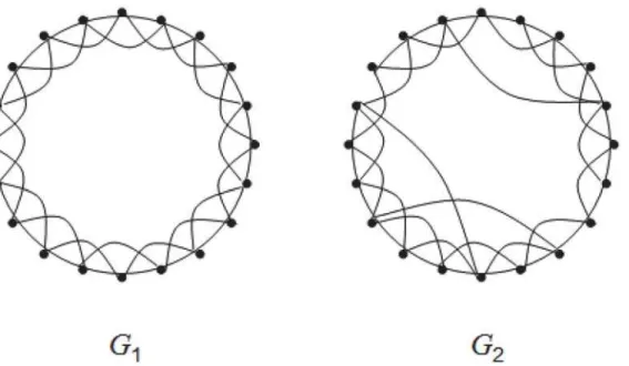
We consider a random evolving networkG1,G2(seeFig. 1), which is introduced in a seminal

paper by Watts and Strogatz [52]. This network is often called WS small-world model, which enables the exploration of intermediate settings between purely local and purely global mixing. As demonstrated in [52], when the rewiring probability is taken around 0.01 (as we considered here), the model is highly clustered, like regular lattices, yet has small characteristic path lengths, like random graphs. This qualitative phenomenon is prevalent in a range of networks arising in nature and technology [53].

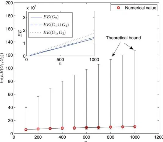
Fig. 2shows the variations of the (dynamic) Estrada indices with the network sizen. The re-sults gathered inFig. 2allow us to draw several interesting comments. First, as expected from the mathematical result [18, Prop. 4], the numerical values ofEE(G1,G2) lie between our

gener-al upper and lower bounds (remarkably much closer to one than the other; see the main panel). Second, both the Estrada index and the dynamic Estrada index grow gradually as the network size increases. Third, the Estrada indicesEE(G2) andEE(G1[G2) are close to each other.

How-ever, both of them are significantly smaller than the dynamic Estrada indexEE(G1,G2),

under-scoring the relevance of dynamic Estrada index—neither the static snapshot graph nor the

aggregated graph constitutes a reasonable approximation to the evolving graph itself.

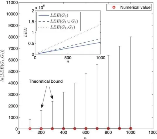
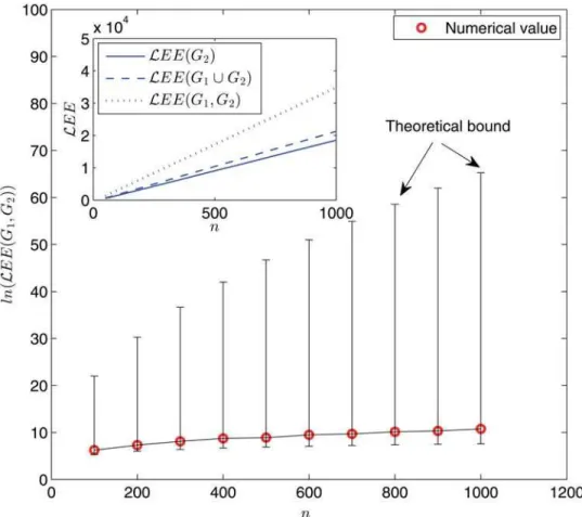
InFig. 3andFig. 4, we display the variations of the (dynamic) Laplacian Estrada indices and the (dynamic) normalized Laplacian Estrada indices, respectively, with the network size. Anal-ogous observations can be drawn. For example, the behavior ofLEE(G1,G2) (andLEE(G1,G2))

differentiates from that ofLEE(G2) (andLEE(G2)) orLEE(G1[G2) (andLEE(G1[G2))

dra-matically. Moreover, when comparingFig. 2withFig. 3andFig. 4, we see that the difference

Fig 1. Illustration of an evolving small-world graphG₁,G₂.G1is a ring lattice over a vertex setVof sizen. It is a 4-regular graph, where each vertex is connected to its 4 nearest neighbors.G2is obtained by rewiring each edge—i.e., choosing a vertexv2Vand an incident edge, reconnecting the edge to a vertex that is not a neighbor ofv—with probabilityp= 0.01 uniformly at random. In the simulations below, we taken₂[100, 1000].

between dynamic and static cases turns out to be much more prominent in the Laplacian ma-trix and normalized Laplacian mama-trix settings than the adjacency mama-trix setting. For example, when the network size is taken asn= 1000, the differencejEE(G1,G2)−EE(G1[G2)j

4 × 103; butjLEE(G1,G2)−LEE(G1[G2)j 7 × 105andjLEE(G1,G2)−LEE(G1[G2)j

1.4 × 104.

Two remarks are in order. First, the theoretical upper and lower bounds for all the three dy-namic Estrada indices shown in Figs.2,3, and4are fairly far apart, due to the fact that our bounds are general and valid for all graphs. This is similar to the situation of static graph case, see [12]. Thus, it would be interesting to identify the specific locations of concrete graphs (such as the WS small-world model studied here) in the spectrum. Second, extensive simulations have been performed for some different values of rewiring probabilitypand ring lattice degree

k, all yielding quantitatively similar phenomena.

Fig 2. Logarithm of the dynamic Estrada index ln(EE(G₁,G₂)) as a function of network sizen.Main panel: numerical results (red circles) and theoretical bounds (upper and lower bars) given by [18, Prop. 4]. Each data point is obtained for one network sample. Inset: simulation results forEE(G1,G2) (dotted line),EE

(G1[G2) (dashed line), andEE(G2) (solid line) via an ensemble averaging of 100 independent random network samples.

Conclusion

A combined theoretical and computational analysis of the dynamic Estrada indices for evolving graphs has been performed. Following the dynamic Estrada index [18], (i) we investigated the dynamic Laplacian Estrada index and the dynamic normalized Laplacian Estrada index, whose mathematical properties such as the upper and lower bounds are established in general settings; (ii) the relations between bounds of these three dynamic Estrada indices are explored; (iii) the remarkable difference between static and dynamic indices are appreciated through numerical simulations for evolving random small-world networks.

The emergence of vast time-dependent networks in a range of fields demands the transition of analytic techniques from static graphs to evolving graphs. Many of these methods were re-viewed in the surveys [2,10]. We expect that the results developed in this paper can be used to evaluate various aspects of structure (in terms of graph spectra) and performance (such as ro-bustness) of evolving networks. Some recent works relevant to the topic of Estrada index can be found in, e.g., [54–58].

Fig 3. Logarithm of the dynamic Laplacian Estrada index ln(LEE(G₁,G₂)) as a function of network size

n.Main panel: numerical results (red circles) and theoretical bounds (upper and lower bars) given by Proposition 2. Each data point is obtained for one network sample. Inset: simulation results forLEE(G1,G2) (dotted line),LEE(G1[G2) (dashed line), andLEE(G2) (solid line) via an ensemble averaging of 100 independent random network samples.

Acknowledgments

The author thank the anonymous reviewers for the helpful comments on the manuscript.

Author Contributions

Conceived and designed the experiments: YS. Performed the experiments: YS. Analyzed the data: YS. Contributed reagents/materials/analysis tools: YS. Wrote the paper: YS.

References

1. Grindrod P, Higham DJ. Evolving graphs: dynamical models, inverse problems and propagation. Proc R Soc A Math Phys Eng Sci. 2010; 466: 753–770. doi:10.1098/rspa.2009.0456

2. Holme P, Saramöki J. Temporal networks. Phys Rep. 2012; 519: 97–125. doi:10.1016/j.physrep. 2012.03.001

3. Grindrod P, Parsons MC, Higham DJ, Estrada E. Communicability across evolving networks. Phys Rev E. 2011; 83: 046120. doi:10.1103/PhysRevE.83.046120

4. Estrada E. Characterization of 3D molecular structure. Chem Phys Lett. 2000; 319: 713–718. doi:10. 1016/S0009-2614(00)00158-5

Fig 4. Logarithm of the dynamic normalized Laplacian Estrada index ln(LEE(G₁,G₂)) as a function of network sizen.Main panel: numerical results (red circles) and theoretical bounds (upper and lower bars) given by Proposition 5. Each data point is obtained for one network sample. Inset: simulation results forLEE

(G1,G2) (dotted line),LEE(G1[G2) (dashed line), andLEE(G2) (solid line) via an ensemble averaging of 100 independent random network samples.

5. Estrada E. Characterization of the folding degree of proteins. Bioinformatics. 2002; 18: 697–704. doi: 10.1093/bioinformatics/18.5.697PMID:12050066

6. Estrada E, Rodríguez-Velázquez JA, RandićM. Atomic branching in molecules. Int J Quantum Chem. 2006; 106: 823–832. doi:10.1002/qua.20850

7. Estrada E, Rodríguez-Velázquez JA. Subgraph centrality in complex networks. Phys Rev E. 2005; 71: 056103. doi:10.1103/PhysRevE.71.056103

8. Estrada E, Rodríguez-Velázquez JA. Spectral measures of bipartivity in complex networks. Phys Rev E. 2005; 72: 046105. doi:10.1103/PhysRevE.72.046105

9. Shang Y. Perturbation results for the Estrada index in weighted networks. J Phys A Math Theor. 2011; 44: 075003. doi:10.1088/1751-8113/44/7/075003

10. Estrada E, Hatano N, Benzi M. The physics of communicability in complex networks. Phys Rep. 2012; 514: 89–119. doi:10.1016/j.physrep.2012.01.006

11. de la Peñna JA, Gutman I, Rada J. Estimating the Estrada index. Linear Algebra Appl. 2007; 427: 70–

76. doi:10.1016/j.laa.2007.06.020

12. Gutman I, Deng H, RadenkovićS. The Estrada index: an updated survey. In: CvetkovićD, Gutman I, editors. Selected Topics on Applications of Graph Spectra. Beograd: Math Inst; 2011. pp. 155–174. 13. Wu J, Barahona M, Tan Y, Deng H. Robustness of random graphs based on graph spectra. Chaos.

2012; 22: 043101. doi:10.1063/1.4754875PMID:23278036

14. Wu J, Barahona M, Tan Y, Deng H. Natural connectivity of complex networks. Chin Phys Lett. 2010; 27: 078902. doi:10.1088/0256-307X/27/7/078902

15. Shang Y. Local natural connectivity in complex networks. Chin Phys Lett. 2011; 28: 068903. doi:10. 1088/0256-307X/28/6/068903

16. Shang Y. Biased edge failure in scale-free networks based on natural connectivity. Indian J Phys. 2012; 86: 485–488. doi:10.1007/s12648-012-0084-4

17. Shang Y. Random lifts of graphs: network robustness based on the Estrada index. Appl Math E-Notes. 2012; 12: 53–61.

18. Shang Y. The Estrada index of evolving graphs. Appl Math Comput. 2015; 250: 415–423. doi:10. 1016/j.amc.2014.10.129

19. Chung FRK. Spectral Graph Theory. Providence: American Mathematical Society; 1997.

20. Cvetković_{D, Doob M, Sachs H. Spectra of Graphs—Theory and Application. Heidelberg: Barth; 1995} 21. Fath-Tabar GH, Ashrafi AR, Gutman I. Note on Estrada and L-Estrada indices of graphs. Bull Acad

Serbe Sci Arts (Cl Math Natur). 2009; 34: 1–16.

22. Li J, Guo J, Shiu WC. The normalized Laplacian Estrada index of a graph. Filomat. 2014; 28: 365–371. doi:10.2298/FIL1402365L

23. Estrada E. Communicability in temporal networks. Phys Rev E. 2013; 88: 042811. doi:10.1103/ PhysRevE.88.042811

24. Grindrod P, Higham DJ. A matrix iteration for dynamic network summaries. SIAM Rev. 2013; 55: 118–

128. doi:10.1137/110855715

25. Grindrod P, Stoyanov ZV, Smith GM, Saddy JD. Primary evolving networks and the comparative analy-sis of robust and fragile structures. J Complex Networks. 2014; 2: 60–73. doi:10.1093/comnet/cnt015 26. Grindrod P, Higham DJ. A dynamical systems view of network centrality. Proc R Soc A Math Phys Eng

Sci. 2014; 470: 20130835. doi:10.1098/rspa.2013.0835

27. Shang Y. Multi-agent coordination in directed moving neighborhood random networks. Chin Phys B. 2010; 19: 070201. doi:10.1088/1674-1056/19/7/070201

28. Li Q, Lqbal A, Perc M, Chen M, Abbott D. Coevolution of quantum and classical strategies on evolving random networks. PLoS One. 2013; 8: e68423. doi:10.1371/journal.pone.0068423PMID:23874622 29. Wu B, Zhou D, Fu F, Luo Q, Wang L, Traulsen A. Evolution of cooperation on stochastic dynamical

net-works. PLoS One. 2010; 5: e11187. doi:10.1371/journal.pone.0011187PMID:20614025

30. Shang Y. Estrada index of general weighted graphs. Bull Aust Math Soc. 2013; 88: 106–112. doi:10. 1017/S0004972712000676

31. Li J, Shiu WC, Chang A. On the Laplacian Estrada index of a graph. Appl Anal Discrete Math. 2009; 3: 147–156. doi:10.2298/AADM0901147L

32. Huang F, Li X, Wang S. On maximum Laplacian Estrada indices of trees with some given parameters. MATCH Commun Math Comput Chem. 2015; 74: in press

34. Chen X, Hou Y. Some Results on Laplacian Estrada Index of Graphs. MATCH Commun Math Comput Chem. 2015; 73: 149–162.

35. Hakimi-Nezhaad M, Hua H, shrafi AR, Qian S. The normalized Laplacian Estrada index of graphs. J Appl Math Informatics. 2014; 32: 227–245. doi:10.14317/jami.2014.227

36. Shang Y. More on the normalized Laplacian Estrada index. Appl Anal Discrete Math. 2014; 8: 346–

357. doi:10.2298/AADM140724011S

37. Kuang J. Applied Inequalities. Jinan: Shandong Science and Technology Press; 2004. 38. Bellman R. Introduction to Matrix Analysis. New York: McGraw-Hill; 1970.

39. Gutman I, Das KC. The first Zagreb index 30 years after. MATCH Commun Math Comput Chem. 2004; 50: 83–92.

40. Shang Y. Lower bounds for the Estrada index using mixing time and Laplacian spectrum. Rocky Moun-tain J Math. 2013; 43: 2009–2016. doi:10.1216/RMJ-2013-43-6-2009

41. Zhou B, Gutman I. More on the Laplacian Estrada index. Appl Anal Discrete Math. 2009; 3: 371–378. doi:10.2298/AADM0902371Z

42. Li X, Shi Y, Gutman I. Graph Energy. New York: Springer; 2012.

43. Huo B, Li X, Shi Y. Complete solution to a conjecture on the maximal energy of unicyclic graphs. Euro-pean J Combin. 2011; 32: 662–673. doi:10.1016/j.ejc.2011.02.011

44. Gutman I, Zhou B. Laplacian energy of a graph. Linear Algebra Appl. 2006; 414: 29–37. doi:10.1016/j. laa.2005.09.008

45. Huo B, Li X, Shi Y. Complete solution to a problem on the maximal energy of unicyclic bipartite graphs. Linear Algebra Appl. 2011; 434: 1370–1377. doi:10.1016/j.laa.2010.11.025

46. Bollobás B, Erdős P. Graphs of extremal weights. Ars Combin. 1998; 50: 225–233

47. Hu Y, Li X, Shi Y, Xu T, Gutman I. On molecular graphs with smallest and greatest zeroth-order general Randić_{index. MATCH Commun Math Comput Chem. 2005; 54: 425–434.}

48. Hu Y, Li X, Shi Y, Xu T. Connected (n,m)-graphs with minimum and maximum zeroth-order general Randićindex. Discrete Appl Math. 2007; 155: 1044–1054. doi:10.1016/j.dam.2006.11.008

49. Wang CL. On development of inverses of Cauchy and Hölder inequalities. SIAM Rev. 1979; 21: 550–

557. doi:10.1137/1021096

50. Cavers M. The normalized Laplacian matrix and general Randić_{index of graphs. Ph.D. Thesis,} Univer-sity of Regina. 2010.

51. Li X, Shi Y. A survey on the Randićindex. MATCH Commun Math Comput Chem. 2008; 59: 127–156. 52. Watts DJ, Strogatz SH. Collective dynamics of‘small-world’networks. Nature. 1998; 393: 440–442.

doi:10.1038/30918PMID:9623998

53. Albert R, Barabási A-L. Statistical mechanics of complex networks. Rev Mod Phys. 2002; 74: 47–97. doi:10.1103/RevModPhys.74.47

54. Gao N, Qiao L, Ning B, Zhang S. Coulson-type integral formulas for the Estrada index of graphs and the skew Estrada index of oriented graphs. MATCH Commun Math Comput Chem. 2015; 73: 133–

148.

55. Chen L, Shi Y. Maximal matching energy of tricyclic graphs. MATCH Commun Math Comput Chem. 2015; 73: 105–119.

56. Chen X, Qian J. On resolvent Estrada index. MATCH Commun Math Comput Chem. 2015; 73: 163–

174.

57. Gutman I, Furtula B, Chen X, Qian J. Graphs with smallest resolvent Estrada indices. MATCH Commun Math Comput Chem. 2015; 73: 267–270.