Locating Eigenvalues of Perturbed Laplacian Matrices of Trees
†R.O. BRAGA1* and V.M. RODRIGUES2
Received on December 1, 2016 / Accepted on May 17, 2017
ABSTRACT.We give a linear time algorithm to compute the number of eigenvalues of any perturbed Laplacian matrix of a tree in a given real interval. The algorithm can be applied to weighted or unweighted trees. Using our method we characterize the trees that have up to 5 distinct eigenvalues with respect to a family of perturbed Laplacian matrices that includes the adjacency and normalized Laplacian matrices as special cases, among others.
Keywords:perturbed Laplacian matrix, eigenvalue location, trees.
1 INTRODUCTION
TheSpectral Graph Theorystudies the relations between the spectrum of matrices associated to graphs and structural properties of the graphs. The most commonly used representation matrix of a graph is theadjacency matrix. IfGis a simple undirected graph with verticesv1, v2, . . . , vn,
the adjacency matrixA=(ai j)ofGis the real symmetric matrix of ordernwith entries 0 or 1,
whereai j =1 if and only if verticesvi andvj are adjacent.
Atree is a connected graph with no cycles. In 2011, Jacobs & Trevisan [7] gave a linear time algorithm to compute the number of eigenvalues of a tree in a given real interval. Their method has the important advantage of being executed directly on the tree so that the matrix is not needed explicitly. The authors observed that the algorithm had potential to be adapted to other matrices, for instance theLaplacian matrix, defined as the matrixL =DG−A, whereDGis the diagonal
matrix whose diagonal entryiiis the degreedi of vertexvi of a graphGandAis the adjacency
matrix ofG.
In fact, the algorithm of Jacobs and Trevisan and the extensions that followed it became a prac-tical and efficient tool in Spectral Graph Theory. We notice in particular the work of Fritscher
†This work was presented at CNMAC 2016, Brazil.
*Corresponding author: Rodrigo Orsini Braga – E-mail: [email protected]
1This work is part of the doctoral studies of this author. Departamento de Matem´atica Pura e Aplicada, IME – UFRGS, Av. Bento Gonc¸alves, 9500, 91509-900 Porto Alegre, RS, Brasil.
et al. [5], where the original algorithm was adapted for the Laplacian matrix of a tree and ap-plied to prove that among all trees withnvertices, the starSnhas the highestLaplacian energy,
which was conjectured by Radenkovi´c & Gutman in [8]. Besides, Braga et al. [3] adapted the original algorithm for thenormalized Laplacian matrix, introduced by Chung [4] as the matrix L=(ℓi j), whereℓi j =1 ifi = janddi >0,ℓi j = −√1
di·dj, if vertices
vi andvj are adjacent,
andℓi j =0, otherwise. This variation of the algorithm was used to study the multiplicity of
nor-malized Laplacian eigenvalues of small diameter trees, which allowed the authors to characterize the trees that have up to 5 distinct normalized Laplacian eigenvalues.
The results obtained with the localization algorithm for different representation matrices of trees motivated the development of an algorithm to localize the eigenvalues of a tree for a more general class of matrices, generalizing the previous algorithms, which is the aim of this work.
Aweighted graphis a graph where a real number ω(ei j) = ωi j is assigned to each edgeei j
connecting verticesvi andvj. We say thatωi j is theweightof edgeei j. An unweighted graph
can be considered as a graph where all edges have weight 1. In [1], Bapat et al. defined the perturbed Laplacian matrixof a graph with positive weights, which encompasses the adjacency, Laplacian and normalized Laplacian matrices, among others. Given a real diagonal matrix D, the perturbed Laplacian matrix ofGwith respect toD, is the matrix
L
D(G)
=D−A,
whereA=(ai j)is the adjacency matrix ofG, withai j =ωi j if verticesvi andvj are adjacent,
and 0 otherwise.
The general idea of the localization algorithm for a perturbed Laplacian matrix of a weighted tree, calledDiagonalizeW, is the same of the previous algorithms: performing computations directly on the tree, obtain a diagonal matrix Dα congruent to M +αI, where M is a representation
matrix of a tree.
Beyond preserving the practicality of the original algorithm and its extensions, our method has the advantages of considering weighted trees and allowing to simultaneously derive results for several representation matrices. In fact, the previous localization algorithms are special cases of algorithmDiagonalizeW. For an unweighted tree, ifDis the zero matrix thenDL(G)= −A andDiagonalizeWcoincides with the algorithm given in [7]. IfDis the diagonal matrix of the degrees of the vertices ofG, thenDL(G)is the Laplacian matrix ofGandDiagonalizeWcoincides with the algorithm applied in [5]. Besides, ifDis the identity matrix and we takeωi j =√1
di·dj, DiagonalizeWis the algorithm for the normalized Laplacian matrix given in [3].
2 LOCATING EIGENVALUES OF PERTURBED LAPLACIAN MATRICES
Taking as input a weighted treeT of ordern, a scalarα ∈Rand a real diagonal matrixD, the algorithmDiagonalizeW(T, α)that we present in this section diagonalizes the matrixDL(T)+αI, whereDL(T)is the perturbed Laplacian matrix ofT with respect to D. The output is a diagonal matrixDα congruenttoDL(T)+αI. We recall that two square matrices of ordern,AandB, are
congruent if there is an invertible matrixPsuch that A= PTB P.
Like the original algorithm of Jacobs and Trevisan for the adjacency matrix, our method is exe-cuted directly on the treeT, so that the matrix is not needed explicitly.
The treeT is rooted at an arbitrary vertex and the vertices are orderedv1, . . . , vn, so that ifvj is
a child ofvk, then j>k. Thus the root is the vertexv1. Every vertexvofT, except for the root,
has aparent, which is the vertex adjacent tovthat is not a child ofv.
During the execution the algorithmDiagonalizeW(T, α)assigns, to each vertexvi ofT, a real
valuea(vi)which at the end corresponds precisely to the entryii of the diagonal matrix Dα.
We call a(vi)thediagonal value of vertex vi. Initially, each vi receives the diagonal value
a(vi)=δi+α, whereδiis the entryii of the diagonal matrixD. Then the vertices are processed
bottom-up, towards the root, as described below. For a vertexvk, we denote byCk the set of all
children ofvk. Ifvkis a leaf which is not the root, thenCk= ∅.
Algorithm 1-DiagonalizeW(T, α).
Input: weighted treeT with ordered verticesv1, v2, . . . , vn, scalarα, diagonal matrixD.
Output: diagonal matrixDαcongruent toDL(T)+αI.
Initializea(vi):=δi+α, for each vertexvi.
Fork=nto 1
ifvkis not a leaf then
1. ifa(vi)=0, for allvi ∈Ck, then
a(vk)←a(vk)−
vi∈Ck
(ωik)2
a(vi)
.
2. ifa(vi)=0 for somevi ∈Ck, then
select one vertexvjinCk for whicha(vj)=0;
a(vk)← −
(ωj k)2
2 ; a(vj)←2;
ifvkhas a parentvℓ, remove the edgevkvℓ.
To understand how the procedure above computes the diagonal values of a diagonal matrix con-gruent to the matrixDL(T)+αI, let us consider a vertexvkofTwith a childvj, which corresponds
to the entries in the matrix below:
k j ⎡ ⎢ ⎢ ⎢ ⎢ ⎢ ⎢ ⎢ ⎢ ⎣ .. . ...
· · · a(vk) . . . ωk j · · ·
..
. . .. ...
· · · ωj k · · · a(vj) · · ·
.. . ... ⎤ ⎥ ⎥ ⎥ ⎥ ⎥ ⎥ ⎥ ⎥ ⎦ .
Ifa(vj)=0, then the following row and column operations annihilate the entriesk j andj k:
Rk ←Rk −
ωj k
a(vj)
Rj and Ck ←Ck−
ωj k
a(vj)
Cj.
After these two operations, the corresponding entries of the matrix are
k j ⎡ ⎢ ⎢ ⎢ ⎢ ⎢ ⎢ ⎢ ⎢ ⎢ ⎣ .. . ...
· · · a(vk)−(ωk j)
2
a(vj) . . . 0 · · ·
..
. . .. ...
· · · 0 · · · a(vj) · · ·
.. . ... ⎤ ⎥ ⎥ ⎥ ⎥ ⎥ ⎥ ⎥ ⎥ ⎥ ⎦ .
Note that ifvk has all children with nonzero diagonal values, each of them may be used to
annihilate the two off-diagonal entries that correspond to its connection withvk. Hence, after
performing the same operations for all children ofvk, the diagonal value ofvkbecomes
a(vk)−
vi∈Ck
(ωik)2
a(vi)
,
which corresponds to the value assigned by Algorithm 1 in this case (Step 1).
Suppose thatvkhas a childvj witha(vj)=0, as in the submatrix below. Then vertex vj may
be used to annihilate the two off-diagonal entries of any other child vi ofvk, as well as the
two entries representing the edge betweenvkand its parentvℓ, in the casevk is not the root, as
follows. Note that at this pointvkandvℓstill have their initial diagonal values, since the vertices
are processed bottom-up.
ℓ k j i ⎡ ⎢ ⎢ ⎢ ⎣
δℓ+α ωℓk
ωkℓ δk+α ωk j ωki
ωj k 0
ωik a(vi)
The operations
Ri ← Ri−
ωik
ωj k
Rj and Ci ←Ci −
ωki
ωk j
Cj,
annihilate the entriesikandki, while the operations below annihilate the entriesℓkandkℓ:
Rℓ ←Rℓ −
ωℓk
ωj k
Rj and Cℓ←Cℓ−
ωkℓ
ωk j
Cj.
Note thatωj k =ωk j =0, sincevj is a child ofvk.
These last two operations effectively remove the edge betweenvkand its parentvℓ, disconnecting
the graph, which is performed in Step 2 of Algorithm 1. At this point, the submatrix with rows and columnsi,j,k, ℓhas been transformed as
ℓ k j i ⎡ ⎢ ⎢ ⎢ ⎣
δℓ+α 0
0 δk+α ωk j 0
ωj k 0
0 a(vi)
⎤ ⎥ ⎥ ⎥ ⎦ .
Next, the operations
Rk ← Rk−
(δk +α)
2ωj k
Rj and Ck ←Ck−
(δk+α)
2ωk j
Cj
annihilate the entrykkand the submatrix becomes
ℓ k j i ⎡ ⎢ ⎢ ⎢ ⎣
δℓ+α 0
0 0 ωk j 0
ωj k 0
0 a(vi)
⎤ ⎥ ⎥ ⎥ ⎦ .
Finally, the operations
Rj ← Rj+ω1k jRk, Cj ← Cj+ω1j kCk,
Rk ← Rk−
ωk j
2 Rj, Ck ← Ck−
ωj k
2 Cj
yield the diagonalized form
ℓ k j i ⎡ ⎢ ⎢ ⎢ ⎣
δℓ+α 0
0 −(ωk j)
2
2 0 0
0 2
0 a(vi)
⎤ ⎥ ⎥ ⎥ ⎦ .
The diagonal values ofvj andvk obtained after the operations above are exactly the values
di-rectly assigned by the algorithm in Step 2. We also note that all other children ofvkare unaffected
Considering that the diagonal values computed by algorithmDiagonalizeW(T, α)were obtained by elementary row and column operations, such that each operation performed in one row was also performed in the corresponding column, it follows that the diagonal matrix Dα, whose
entries are the diagonal values assigned by the algorithm, is congruent toDL(T)+αI. Therefore, by Sylvester’s Law of Inertia (see [6, Theorem 4.5.8]), we have the next result.
Theorem 2.1. Given a real diagonal matrix D, let Dα be the diagonal matrix produced by the
algorithm DiagonalizeW(T,−α)for a weighted tree T and real numberα. Then, the number of positive, negative and zero diagonal entries in Dα is equal to the number of eigenvalues of the
perturbed Laplacian matrix of T with respect to D, LD(T), which are greater, smaller and equal toα, respectively.
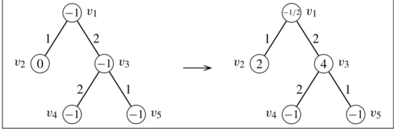
Example 2.2. LetT be the weighted tree with verticesv1, v2, v3, v4andv5on the left side of
Figure 1, with weights represented on the edges. Suppose that the diagonal entries of matrixD areδ1=1, δ2=2, δ3=1, δ4=1 andδ5=1.
Let us apply algorithmDiagonalizeW(T, α), withα= −2. The initial diagonal values assigned to the vertices area(vi)=δi−2, fori =1, . . . ,5, which are represented on the vertices ofT,
on the left side of Figure 1.
−1 v1
0
v2 −1 v3
−1
v4 −1 v5
1 2
2 1
−1/2 v1
2
v2 4 v3
−1
v4 −1 v5
1 2
2 1
Figure 1: AlgorithmDiagonalizeW(T, α)withα= −2.
Verticesv4andv5are the children ofv3and have nonzero values, hence the algorithm assigns
a(v3)= −1−(ω34)
2
a(v4) − (ω35)2
a(v5) = −
1− 2
2
−1 − 12 −1 =4.
Vertex v1 has a child with a zero value (vertexv2), then the algorithm assigns value 2 tov2,
whereas the diagonal value ofv1becomes
a(v1)= − (ω12)2
2 = −
12
2 = −
1 2.
and four positive eigenvalues, while withα= −1 we get thatDL(T)has one eigenvalue equal to 1, two eigenvalues smaller than 1 and two eigenvalues greater than 1. Hence,DL(T)has one negative eigenvalue, one eigenvalue in the interval(0,1), one eigenvalue equal to 1 and two eigenvalues greater than 2.
3 TREES WITH AT MOST FIVE DISTINCT EIGENVALUES WITH RESPECT A FAMILY OF PERTURBED LAPLACIAN MATRICES
In this section we apply AlgorithmDiagonalizeW(T, α)to study trees that have up to 5 distinct perturbed Laplacian eigenvalues.
It follows from the Theorem below, whose proof can be found in [2, Proposition 1.3.3], that we only need to consider trees with a small diameter. We recall that thediameterof a graph is the maximum distance between any two vertices in the graph.
Theorem 3.1. If G is a connected graph with diameter d and M = (mi j)is a nonnegative
symmetric matrix with rows and columns indexed by the vertices of G and such that for distinct verticesvi, vj we have mi j >0if and only ifvi andvj are adjacent, then G has at least d+1
distinct eigenvalues with respect to M.
We show next that this property is more general. For that matter we apply a result due to Schur, whose proof can be found in [6, Theorem 4.3.45].
Theorem 3.2 (Schur).Let A be a real symmetric matrix of order n with diagonal entries d1 d2. . .dnand eigenvaluesλ1λ2. . .λn. Then
k
i=1 di
k
i=1
λi, for k=1, . . . ,n−1, and n
i=1 di =
n
i=1 λi.
Theorem 3.3. If G is a connected graph with positive weights and diameter d, then any per-turbed Laplacian matrix of G has at least d+1distinct eigenvalues.
Proof. LetGbe a connected graph with ordern, positive weights and diameterd. LetDL(G)= D−Abe the perturbed Laplacian matrix ofGwith respect to a diagonal matrixD=(di j). Let
us denote the entries of the adjacency matrix ofGbyai j, withi,j ∈ {1, . . . ,n}. Let
m=1+ max
1kn{λk},
whereλ1, . . . , λnare the eigenvalues ofDL(G), and consider the matrixB=m I−DL(G)=m I−
D+A. Then, for alli, j ∈ {1, . . . ,n}withi = j,bi j =ai j 0. Besides, for alli∈ {1, . . . ,n},
the diagonal entrybii = m −dii of B is positive. This follows from the fact thatDL(G)is
symmetric and then, by Theorem 3.2,dii max
1kn{λk}<m. Therefore, by Theorem 3.1,Bhas
at leastd+1 distinct eigenvalues. Since the eigenvalues ofBarem−λ1, . . . ,m−λn, it follows
The perturbed Laplacian matrix of a graph depends on an arbitrary diagonal matrixD. We con-sider the case where D=µI, for someµ∈ R, thus the perturbed Laplacian matrix of a graph Gis of the form
L
D(G)
=µI−A.
Note that, in particular, ifµ=0,DL(G)= −A. Besides, ifGhas no isolated vertices,µ=1 and the weights ofGare
ωi j =
1 didj
,
thenDL(G) is the normalized Laplacian matrix ofG′, where G′ is an unweighted graph with the same edges and vertices then G. Hence the adjacency matrix of a weighted graph and the normalized Laplacian matrix of an unweighted graph with no isolated vertices are special cases of a perturbed Laplacian matrix of the formDL(G)=µI−A.
It is known that the spectrum of the adjacency matrix of a connected graphG is symmetric if and only ifGis bipartite (see [2, Proposition 3.4.1]). The family of perturbed Laplacian matrices that we are considering satisfies a similar result. It is easy to see that the spectrum ofµI −Ais symmetric aboutµ∈Rif and only if the spectrum ofAis symmetric. In fact, ifλis an eigenvalue ofµI −A, thenµ−λis an eigenvalue of A. Hence, if the spectrum of Ais symmetric, then
λ−µis also an eigenvalue ofA. Thus,µ−(λ−µ)=2µ−λis an eigenvalue ofµI −A. The converse is similar.
Theorem 3.4. Let G be a connected weighted graph of order n andµ∈R. Then G is bipartite if and only if the spectrum of LD(G)=µI−A is symmetric aboutµ.
In order to characterize the trees that have at most five distinct eigenvalues for perturbed Lapla-cian matrices of the formµI−A, for someµ∈R, by Theorem 3.3 it is enough to consider trees with diameter smaller than five, since every tree is a connected graph. Besides, every treeT is a bipartite graph, so the spectrum ofDL(T)=µI−Ais symmetric aboutµ.
LetT be a tree withnvertices and diameterdless than or equal to 4. Ifd =1,T is the complete graph with two vertices and has two different eigenvalues: µ+ω andµ−ω, whereωis the weight of the edge that connects the vertices.
In the case d = 2, T is the star Sn, that has exactly three distinct eigenvalues, symmetric
about µ, which is an eigenvalue with multiplicity ton−2. To see that, we apply algorithm DiagonalizeW(Sn, α), withα= −µand the vertex with degreen−1 as the root. Since alln−1
pendants ofSnreceive zero diagonal values, the algorithm assigns to the rootvthe diagonal value
−(ωvy∗)
2
2 , wherey∗is a pendant ofvselected to receive value 2. Therefore, exactlyn−2 vertices
have a zero diagonal value at the end of the execution, which implies thatµis an eigenvalue with multiplicity ton−2, by Theorem 2.1.
Now we consider the cased =3. Note that any diameter 3 tree can be seen as two starsSk+1
andSℓ+1, wherek, ℓ1, with an edge linking their centers, as illustrated in Figure 2.
Figure 2: A diameter 3 tree.
Theorem 3.5. Let T be a diameter3 tree. Then all eigenvalues of LD(T) = µI −A, except possibly forµ, are simple. Moreover, LD(T)has exactly four eigenvalues if and only if T = P4, the path with four vertices. Otherwise, LD(T)has exactly five distinct eigenvalues.
Proof. Let T be a diameter 3 tree withn = k+ℓ+2 vertices, as shown in Figure 2. By Theorem 3.3,DL(T)=µI −Ahas at least four distinct eigenvalues. Ifn =4,T is the path P4
andDL(T)has exactly four distinct eigenvalues. Suppose thatn>4 and let us apply the algorithm DiagonalizeW(T, α), withα= −µandT rooted at the vertex withℓpendants. Then all vertices are initialized with a zero value. Since allk pendants of the vertex adjacent to the root have zero values, when this vertex is processed its diagonal value becomes negative and one of itsk pendants receives a positive value. Besides, sinceℓ1, the root has at least one pendant with a zero value. Hence, when the algorithm processes the root, its diagonal value becomes negative and exactly one of itsℓpendants receives a positive value. Therefore, at the end of the execution we obtaink+ℓ−2 =n −4 zero values. By Theorem 2.1, it follows thatµis an eigenvalue ofDL(T)with multiplicityn−4. Then the other four eigenvalues ofDL(T)must be distinct since it has at least four distinct eigenvalues and its spectrum is symmetric aboutµ. Hence,DL(T)has exactly five distinct eigenvalues ifn >4, which concludes the proof.
IfT has diameterd = 4, thenDL(T)has at least five distinct eigenvalues. Hence, the path P4
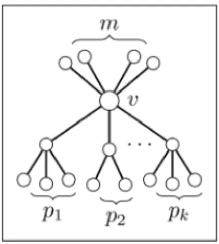
is the only tree with exactly four distinct eigenvalues. We want to characterize the trees, if any, necessarily of diameter 4, that have exactly five distinct eigenvalues for the perturbed Laplacian matrixµI −A. Every diameter 4 tree is of the form depicted in Figure 3: it contains a vertexv
adjacent tok2 verticesv1, . . . , vk, wherevihas degree pi+1, withpi 1, fori =1, . . . ,k,
and eachvi is adjacent topipendants, andvis also possibly adjacent tom0 pendants. In this
case, we writeT =T(k,p1,p2, . . . ,pk,m).
The following result gives the multiplicity ofµas an eigenvalue ofDL(T)=µI−A, whereT is a diameter 4 tree.
Theorem 3.6.For any diameter4tree of the form T =T(k,p1,p2, . . . ,pk,m), the multiplicity
ofµas an eigenvalue ofµI−A is1−k+k
i=1pi 1, when m=0, and m−1−k+ki=1pi,
Figure 3: A diameter 4 treeT(k,p1,p2, . . . ,pk,m).
Proof. Let us apply the algorithmDiagonalizeW(T, α), withα= −µ, toT rooted at vertexv
of degreek+m, which is adjacent to the verticesv1, v2, . . . , vk of degree p1+1, . . . ,pk+1,
respectively.
Suppose thatm=0, that is,vhas no pendants. Sinceµ+α=0, initially all vertices are assigned a zero diagonal value, as the left hand-side of Figure 4 shows. Next, fori=1, . . . ,k, the value of
vi becomes−
(ωv
iv∗i)
2
2 , wherev∗i is a pendant ofvichosen to take value 2, and the edge connecting
vi tovis removed, so that the value of the rootvremains 0. The other(pi−1)pendants also
remain with a zero diagonal value, as illustrated in the right-hand side of Figure 4. Therefore, by Theorem 2.1, the multiplicity ofµas an eigenvalue ofDL(T)=µI −Ais exactly
k
i=1
(pi−1)+1 =
k
i=1 pi
−k+1 1.
0 v
0 0 0
0 0 0 0 0 0 0 0 0
· · ·
0 v
− − −
0 0 + 0 + 0 0 0 +
· · ·
Figure 4: A diameter 4 tree withm=0.
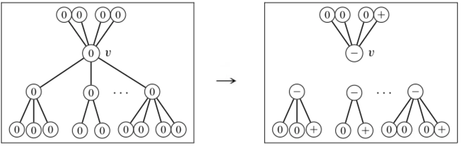
Now suppose thatm >0. Figure 5 illustrates the execution the algorithm in this case. All the edges connecting thevi’s tovare also removed.
When the rootv is processed, since it remains connected only to itsm pendants, which have value 0, the value assigned tov becomes −(ωvv∗)2
2 , wherev∗is a pendant ofv chosen to take
value 2. Hence, by Theorem 2.1, the multiplicity ofµas an eigenvalue ofDL(T)=µI−Ais
k
i=1 pi
0 v
0 0 0
0 0 0 0 0 0 0 0 0
· · ·
0 0 0 0
− v
− − −
0 0 + 0 + 0 0 0 +
· · ·
0 0 0 +
Figure 5: A diameter 4 tree withm>0.
The next result gives the multiplicity of the eigenvalues ofDL(T)= µI −Athat are different fromµfor a diameter 4 treeT. Fori =1, . . . ,k, letωihbe the weight of the edge that connects
vi to its pendantqih, forh=1, . . . ,pi, and letσi =hp=i 1(ωih)2.
Theorem 3.7.Let T =T(k,p1,p2, . . . ,pk,m)be a diameter4tree. Then LD(T)
=µI−A has an eigenvalue different fromµwith multiplicity t 2if and only if t <k and exactly t+1σi′s are equal. Moreover,λ1=µ−√σandλ2=µ+√σ are eigenvalues of LD(T)=µI −A with multiplicity t1ifσi =σ for exactly t+1vi′s.
Proof. Let us suppose thatλ=µis an eigenvalue ofDL(T)with multiplicityt 2. Applying algorithmDiagonalizeW(T,−λ)toT rooted at vertexv of degree k+m, each pendant ofT receives the initial diagonal valueµ−λ=0. Hence,
a(vi)=µ−λ− pi
h=1 (ωih)2
µ−λ =µ−λ− σi
µ−λ,
for all 1i k. Due to the multiplicity ofλ, the algorithm produces exactlyt zero diagonal values. Considering that each pendant ofT has a nonzero diagonal value andt2, thena(vi)=
0 for at least onei, since otherwise the only possible zero diagonal value would bea(v), which contradicts the fact thatt 2. Thus, the only way to obtain exactlytzero diagonal values at the end of the algorithm is thata(vi)= 0 for exactlyt+1vi’s, so that, after processing vertexv,
the diagonal value ofvis negative and one of thoset+1vi’s has a positive diagonal value. This
implies thatt+1k. Besides, for 1i < jk,
a(vi)=a(vj) ⇔ µ−λ−
σi
µ−λ =µ−λ− σj
µ−λ ⇔ σi =σj.
Without loss of generality, now let us suppose that for somet, 1 t < k, there existsσ ∈ R
such thatσi = σ, for alli, 1 i t+1, andσi = σ, fori > t+1. We apply algorithm
DiagonalizeW(T, α)toT rooted at vertexvof degreek+mandα= −λ, whereλ=µ−√σ. Initially all pendants ofT are assigned a diagonal valueµ−λ=√σ, which is positive. Besides, for eachi, 1it+1,vi is assigned a zero value, since
a(vi)=µ−λ−
σi
µ−λ =
Therefore, when vertexvis processed, we obtaina(vj)=2, for exactly one jin{1, . . . ,t+1}
anda(v)= −(ωvvj)
2
2 <0. Hence, at the end of the execution, there are exactlyt zero diagonal
values, which implies thatλ is an eigenvalue ofDL(T)with multiplicityt. The result forλ = µ+√σ follows from the symmetry of the spectrum ofDL(T) = µI − A with respect toµ
(Theorem 3.4).
Corollary 3.1. Ifσi =σj for all1 i < j k, then, except possibly byµ, all eigenvalues of
L
D(T)=µI−A are simple.
The result below characterizes the diameter 4 trees for which the perturbed Laplacian matrix of the formµI −Ahas exactly 5 distinct eigenvalues.
Theorem 3.8. Let T =T(k,p1,p2, . . . ,pk,m)be a diameter4tree. If m=0and k =2, or
m =0, k 3andσi =σj, for all1i < j k, then LD(T)=µI −A has exactly5distinct
eigenvalues. Otherwise, LD(T)has at least6distinct eigenvalues.
Proof. Ifm=0, then, by Theorem 3.6, the multiplicity ofµas an eigenvalue ofDL(T)=µI−A is 1−k+k
i=1pi 1. Hence,DL(T)has exactly 2keigenvalues different fromµ. Ifk =2,
the result is clear, since T has at least 5 distinct eigenvalues by Theorem 3.3. Let us suppose thatk 3. Ifσi = hp=i 1(ωih)2 = σ, for all 1 i k, by Theorem 3.7, λ1 = µ+√σ
and λ2 = µ−√σ are eigenvalues ofDL(T) with multiplicityk−1 1. HenceDL(T) has 2k−(2(k−1))=2 eigenvalues different fromµ,λ1andλ2. These two eigenvalues are simple,
since the spectrum ofDL(T)is symmetric about µ(Theorem 3.4), which shows thatDL(T)has exactly 5 distinct eigenvalues.
However, ifσi = σ, for all 1 i t, for some 2 t < k, andσi = σ, for alli > t, the
multiplicity ofλ1andλ2ist−1. HenceDL(T)has 2(k−t+1)4 eigenvalues different from µ, λ1andλ2, which implies thatDL(T)has at least 7 distinct eigenvalues. If σi = σj,for all
1i < j k, by Corollary 3.1,DL(T)has 2k6 simple eigenvalues different fromµ, which shows thatDL(T)has at least 7 distinct eigenvalues. Finally, ifm>0 andk2, by Theorem 3.6, the multiplicity ofµism−1−k+k
i=1pi 0 andDL(T)has 2k+26 eigenvalues different
fromµ. By Theorems 3.4 and 3.7, it follows thatDL(T)has at least 6 distinct eigenvalues, since
in this case the multiplicity ofµcan be zero.
RESUMO.N´os apresentamos um algoritmo de tempo linear para calcular o n´umero de
au-tovalores de uma matriz laplaciana perturbada qualquer associada a uma ´arvore, num dado intervalo real. Este algoritmo pode ser aplicado a ´arvores com ou sem pesos. Utilizando este
procedimento, obtemos uma caracterizac¸˜ao das ´arvores com at´e cinco autovalores distintos para uma fam´ılia de matrizes laplacianas perturbadas, que inclui a matriz de adjacˆencias e a
matriz laplaciana normalizada como casos particulares, entre outras.
REFERENCES
[1] R.B. Bapat, S.J. Kirkland & S. Pati. The perturbed Laplacian matrix of a graph.Linear and Multilin-ear Algebra,49(2001), 219–242.
[2] A.E. Brouwer & W.H. Haemers. “Spectra of graphs”, Springer, New York, (2012).
[3] R.O. Braga, R.R. Del-Vecchio, V.M. Rodrigues & V. Trevisan. Trees with 4 or 5 distinct normalized Laplacian eigenvalues.Linear Algebra and its Applications,471(2015), 615–635.
[4] F.R.K. Chung. “Spectral Graph Theory”, American Math. Soc., Providence, (1997).
[5] E. Fritscher, C. Hoppen, I. Rocha & V. Trevisan. On the sum of the Laplacian eigenvalues of a tree.
Linear Algebra and its Applications,435(2011), 371–399.
[6] R. Horn & C.R. Johnson. “Matrix Analysis”, Cambridge University Press, (1985).
[7] D.P. Jacobs & V. Trevisan. Locating the eigenvalues of trees.Linear Algebra and its Applications, 434(2011), 81–88.